Article

New Chung-Li Ionosonde in Taiwan: System Description and Preliminary Results

Department of Space Science and Engineering, National Central University, Chung-Li, Taoyuan City 320, Taiwan
*
Author to whom correspondence should be addressed.
Remote Sens. 2022, 14(8), 1913; https://doi.org/10.3390/rs14081913
Submission received: 23 March 2022 / Revised: 10 April 2022 / Accepted: 11 April 2022 / Published: 15 April 2022

Abstract

:
In spite of being interrupted several times in its long history of operation since 1950, the routine observation of the ionosphere with various ionosondes installed at the Chung-Li ionosphere station in Taiwan has been achieved successively for more than seven decades. In this article, the system characteristics of the latest Chung-Li ionosonde and algorithm developed by National Central University for ionogram scaling and true height analysis, which started to routinely operate in 2020, are introduced. The new Chung-Li ionosonde is a pulse radar that transmits a train of short pulses with respective carrier frequencies between 2 and 30 MHz at a frequency separation of 50 kHz. The duration of an entire frequency sweep is 294.13 s, which is divided into 561 frequency channels. The 16-bit complementary code is employed to increase the signal-to-noise of the reflected echoes. The observational range is from 70 to 1221 km with a range resolution of 3.84 km. We developed an algorithm for the Chung-Li ionosonde to automatically scale the ionogram such that the true height profile of the ionospheric electron density can be retrieved. The observed traces of the ordinary wave (O-wave) and extraordinary wave (X-wave) displayed on the ionogram were first identified and separated by using 2-dimensional autocorrelation analysis combined with the image projection method. The true height analysis used stepwise regression. With the help of the International Reference Ionosphere (IRI) model and Quasi-Parabolic Segment (QPS) model, we carried out true height analysis to retrieve the ionospheric electron density profile based on the O-wave trace. An examination showed that the ionospheric parameters (i.e., foF2, h’F2) retrieved from the automatic scaling algorithm were essentially in good agreement with those obtained from manual scaling. The ionosonde-measured foF2 and hmF2 were also compared with the FORMOSAT-7 measurements made with the GPS radio occultation technique. The results show that the correlation coefficient, root mean squared deviation, and mean difference were, respectively, in ranges from 0.878 to 0.93, 0.73 to 1.06 MHz, and −0.43 to −0.26 MHz for foF2 and in ranges from 0.701 to 0.8, 22.39 to 28.45 km, and −9.28 to 11.06 km for hmF2.

1. Introduction

The ionosonde is a vertically incident high-frequency (HF) radar that is used exclusively to monitor the terrestrial ionosphere. Conventionally, the ionosonde was designed as a frequency modulation continuous wave (FMCW) radar that transmits a long chirp pulse with continuously linear frequency modulation in a HF range from about 1 MHz to 30 MHz. The pulse is reflected where the incident wave frequency matches the ionospheric plasma frequency, which is a function of ionospheric electron density. An ionogram traces the virtual height, defined as the product of half of the light speed and echo delay time, of the reflected pulses over their frequency. Because the pulse group velocity, as it approaches the reflection height, is less than the light speed, true height analysis is performed to obtain the ionospheric electron density profile [1]. As a result, the ionospheric parameters of the sublayers can be retrieved. In addition to the FMCW radar, a pulse radar that transmits a sequence of short-duration pulses with respective carrier frequencies between 1 and 30 MHz can also be employed to serve as an ionosonde for ionospheric observation. Once the ionogram is generated by assembling the distribution of the virtual heights of the reflected echoes of the transmitted pulses with incident frequencies, similar to the FMCW radar, the ionospheric electron density profile can be retrieved from the true height analysis and the parameters of the various ionospheric layers can thus be obtained.
True height analysis is one of the core data-analyzing procedures in processing the ionosonde echoes. A number of automatic true height analysis algorithms have been developed and proposed by different groups in the ionospheric community to retrieve the true height profile of the ionospheric electron density from observed traces on an ionogram. For example, ARTIST (Automatic Real-Time Ionogram Scaler with True-height), which is believed to be the most widely used algorithm nowadays, uses the adaptive thresholding algorithm combined with artificial neural networks (ANNA) and hyperbolic curve fitting to remove background noise and identify O-wave and X-wave traces on an ionogram for the determination of the ionospheric parameters [2,3,4,5]. The Dynasonde software is implemented in the VIPIR (Vertical Incidence Pulsed Ionospheric Radars) sounders, which is physics-based modeling in cooperation with a knowledge-based pattern recognition technique to extract traditional ionospheric parameters, such as foF2 and hmF2 [6]. The Autoscala developed at Istituto Nazionale di Geofisica e Vulcanologia (INGV) adopted a correlation-based curve-fitting algorithm to identify and scale the traces of the Es layer, F1 layer, and F2 layer of the ionograms without polarization information [4,7,8,9]. On the basis of an image recognition technique, CADI (Canadian Advanced Digital Ionosonde) uses a fuzzy relation to fit the trace, which allows the automatic extraction of the F-layer parameters [10,11]. Ding et al. [12] used an empirical orthogonal function (EOF) to simulate the electron density profile to scale the ionospheric parameters. On the basis of the image projection method, Jiang et al. [13,14,15] developed an autoscaling algorithm to improve the autoscaling performance of trace identification and ionogram scaling. In this study, with the use of the 2-dimensional autocorrelation function (2DACF) combined with the image-projection method, we developed a new autoscaling algorithm to process the ionogram data to identify and separate the O- and X-waves of the traces for ionospheric parameter scaling. The performances of the 2DACF and projection methods in the foF2 identifications will be also compared and discussed.
The first manually operated FMCW ionosonde was built by National Taiwan University and set up in Taipei in 1950 to routinely monitor the ionosphere over Taiwan. The observed ionograms were manually scaled to provide a contour map of the ionospheric frequency of optimum traffic (FOT) for the use of HF (or short-wave) radio propagation in the Taiwan area. In 1960, the Chung-Li ionosphere station (CL424) (24.968°N, 121.196°E, geomagnetic latitude 15.89°N) was established at Taoyuan by the Ministry of Transportation, and an automatic ionosonde (NBS-C2 model) was implemented at the station to commence the era of continuously automatic routine observation of the ionosphere in Taiwan for more than four decades. During this period from 1960 to 2000, two kinds of ionosondes with better performance were acquired to replace the old ones, which were NBS C2/C4 ionosonde (1966) and KEL IPS-42 ionosonde (1984). However, the routine observation of the ionosphere was interrupted in 2000 owing to the reorganization of the government. After transferring the service of ionospheric monitoring from Chunghwa Telecom Company to the National Communications Commission (NCC), a new ionosonde (TCI 820B Chirp sounder) was procured and set up at the Chung-Li ionospheric station in 2006 to recover the ionospheric routine observation in Taiwan. Ten years later, however, the ionospheric routine observation was stopped again in late 2016 by the NCC. Fortunately, under the auspices of the Central Weather Bureau, Ministry of Transportation in Taiwan, a new type of ionosonde was developed by National Central University (NCU) in 2018 and successfully installed and fully operated at the Chung-Li ionosphere station in April 2020 to recover the routine service of ionospheric observation in Taiwan.
In this article, the system characteristics of the new Chung-Li ionosonde and the algorithm to automatically scale the traces on the ionogram for true height analysis will be described. In Section 2, the system layout of the Chung-Li ionosonde will be introduced. In Section 3, the algorithms of trace scaling and true height analysis will be deliberated. In Section 4, the performance of the new Chung-Li ionosonde in the observations of ionospheric parameters will be examined. Conclusions will be drawn in Section 5.

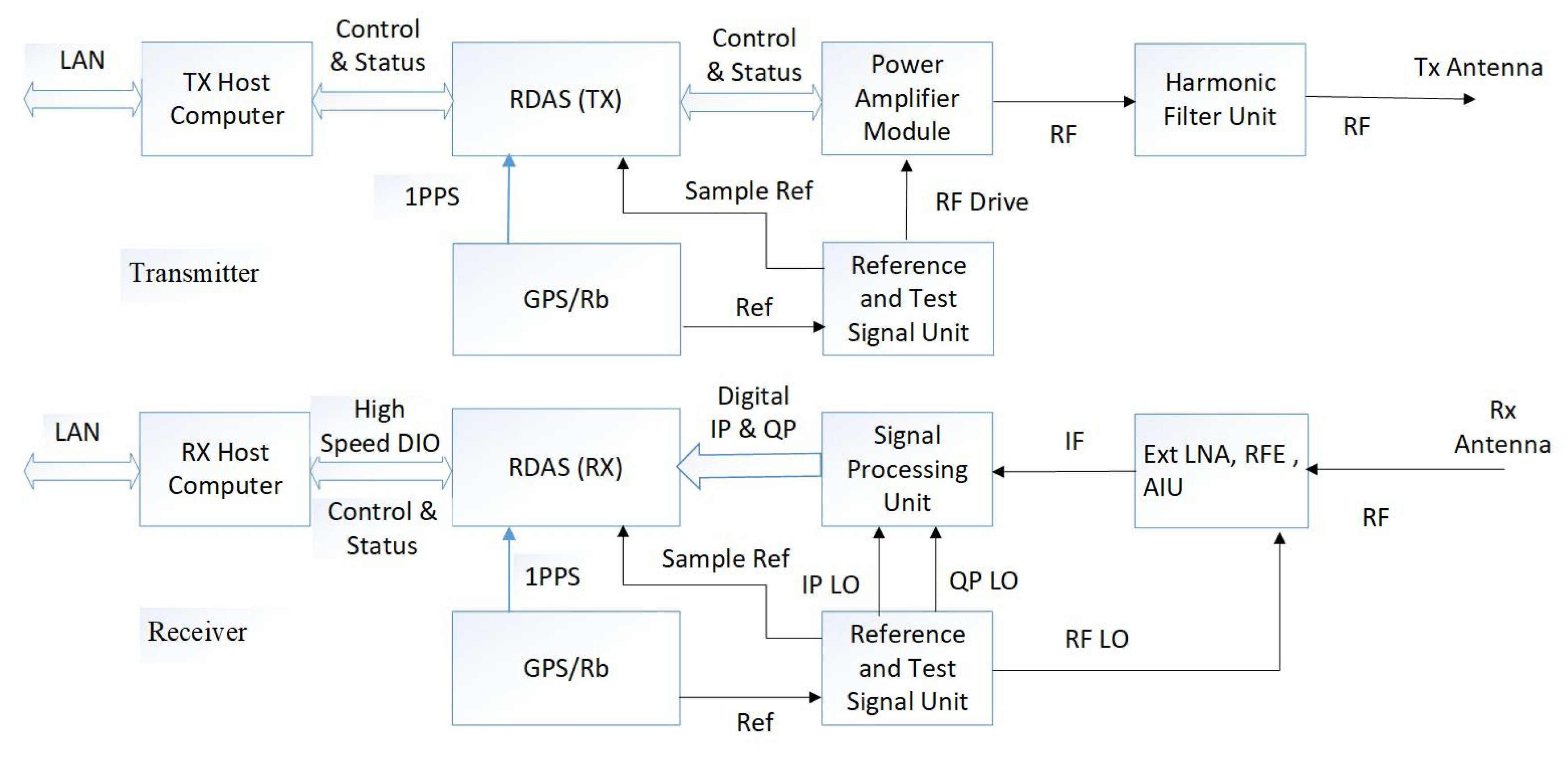
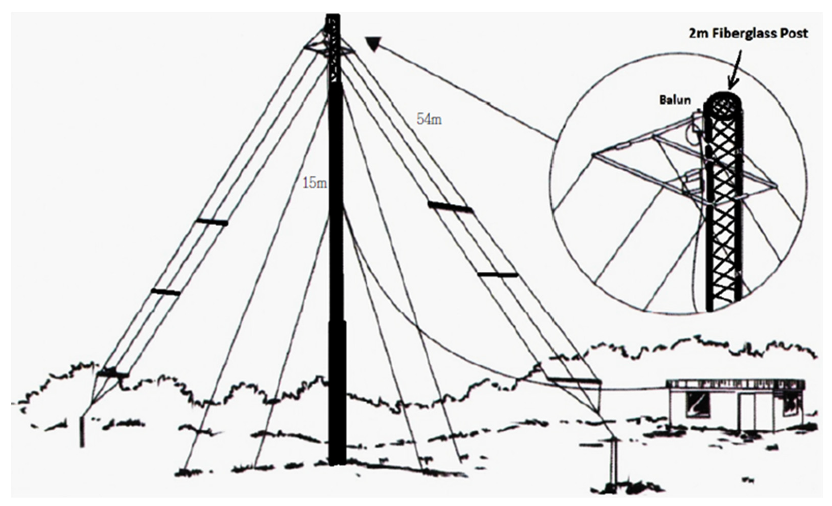
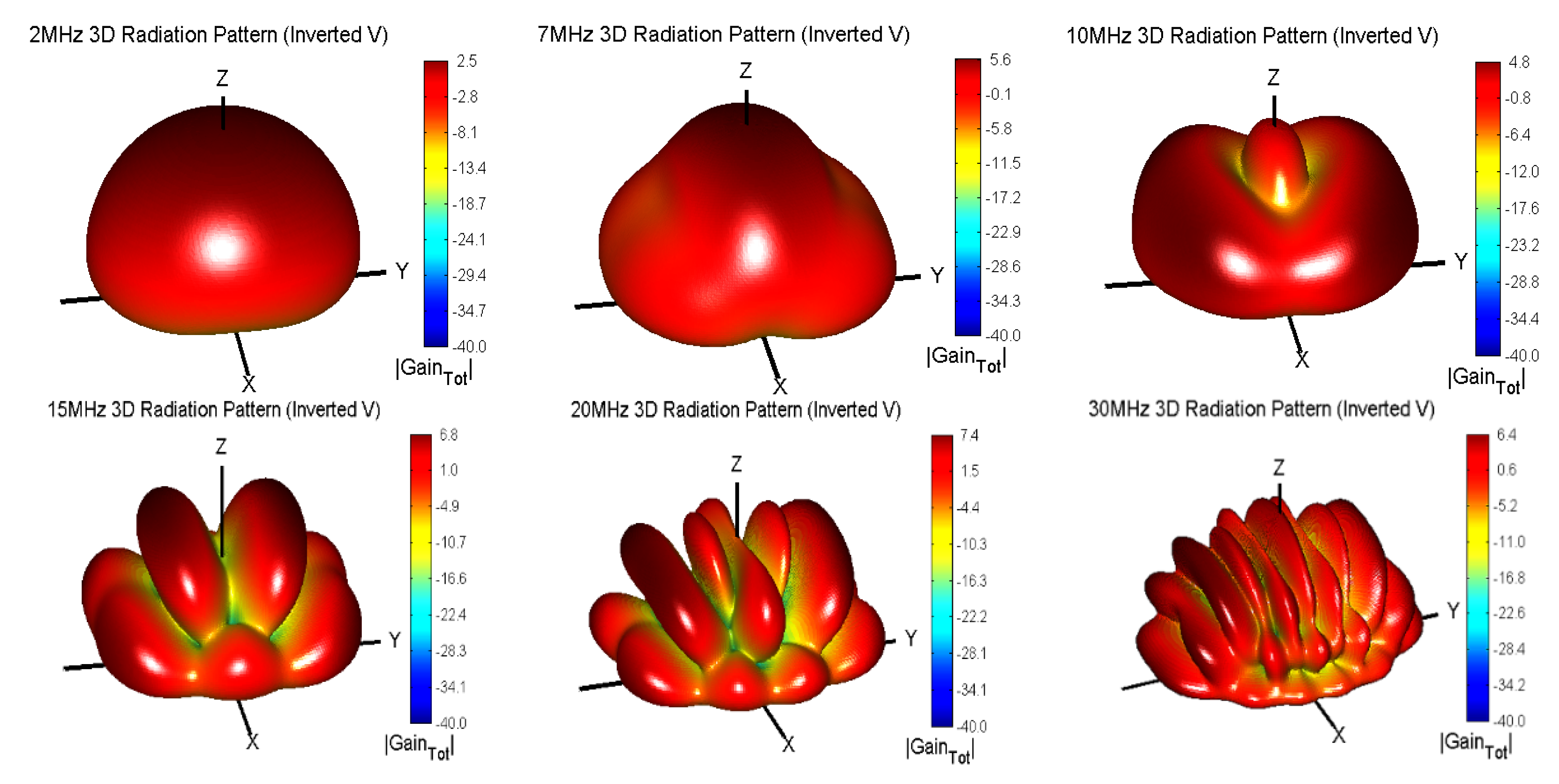
2. System Description

In terms of functional operations, the new Chung-Li ionosonde is classified into two main parts. One part is the radar system that is composed of a transmitter, receiver, antenna, and radar data-acquisition system (RDAS) for transmitting, receiving, and processing radar signals. The other part is the automatic algorithm that is designed to process and scale the ionospheric traces of the reflected radar echoes presented in the ionogram for true height analysis to retrieve the ionospheric electron density profile. The former is primarily manufactured and assembled by the Genesis Software Company based in North Adelaide, Australia, and the latter is developed by National Central University in Taoyuan, Taiwan. Irrespective of a pulse radar, the Chung-Li ionosonde is a bistatic radar system with a transmitter located at the Chung-Li ionosphere station and a receiver situated at Xinwu weather station (25.01°N, 121.04°E) about 15 km northwest of the ionosphere station. In this section, the characteristics of the radar system will be introduced, and the automatic algorithm for ionogram scaling will be described in the next section.
Figure 1 depicts the block diagram of the radar system of the Chung-Li ionosonde, in which the major functional units of the radar system and the primary interconnections between the units are shown. A transmitter with a peak power of 600 W and maximum duty cycle of 7.5% is employed by the Chung-Li ionosonde to emit radar waves in a frequency range of 2–30 MHz. The waveform of the transmitted radar pulse is generated by a direct digital synthesizer (DDS) located in the reference and test signal unit (RTSU). To improve the spectral purity, the transmitted pulses are shaped as trapezoid or Gaussian shapes. The transmitter produces short (12.8 μs) or long (25.6 μs) chip pulses of phase-locked radio frequency (RF) with an inter-pulse period (IPP) of 4096 μs or 8192 μs in the standard mode of operation. A 13-bit Barker code or 16-bit complementary code can be used to increase the average echo power for increased ionospheric detection efficiency. The pulses are emitted from the output port of the harmonic filter unit (HFU), which is designed to drive 50-ohm-load impedances and provide necessary harmonic suppression for main RF signals. Eight harmonic filters are designed as low pass filters with respective frequency responses to suppress the harmonics from the power amplifier to a low level of less than −50 dBc.
The receiving system of the Chung-Li ionosonde is composed of eight units, including a signal processing unit (SPU), reference and test signal unit (RATS), an uninterruptible power supply (UPS), receiver host computer (RXHC), power supply distribution unit (PSDU), radar data-acquisition system (RDAS), antenna interface unit (AIU), and receiver front end (RFE). As shown in Figure 1, the radar returns from the ionospheric reflection detected by the receiving antenna are first fed into a low-noise amplifier (LNA) in RFE to amplify the received radar signals. The LNA output then passes through an eight-channel band-pass filter with the respective center frequency and bandwidth in RFE to suppress out-of-band signals. The ratio between the bandwidth and the center frequency is set properly to render the implementation of the band-pass filter more feasibly. The output of band-pass-filtered signals is split into two identical components and respective frequency down-conversion is performed to generate a pair of in-phase (I) and quadrature (Q) signals at an intermediate frequency (IF). The I/Q signals then enter the data-acquisition module for integration and digitization. The data-acquisition module in the RDAS contains two independent and identical 16-bit digitization channels that serve as analog-to-digital converters (ADC) to sample the analogous base-band I/Q components produced by the receiver down-converters and make the digitized samples available to a set of two signal integration modules. The digitized base-band I/Q signals can be averaged individually between 1 and 4096 times in the data-acquisition module in RDAS under software control, which is referred to as coherent integration. Once coherently integrated data are available, they are transported from the data buffer module in RDAS to the receiver host computer via a high-speed peripheral component interconnect (PCI) bus data link for further analysis. Note that a digitizer and integrator are employed to carry out analog-to-digital conversion (ADC) and the necessary coherent integration to increase the signal-to-noise ratio for better detection. The uninterrupted power supply (UPS) unit is included in the receiver system to provide the necessary power for the functions of RDAS and the host computer. In the event of power failure, the RDAS continues to acquire data, although the transmitter will not continue to transmit. Once the main power is restored, the transmitter will resume transmitting using the factory-set power on the default pulse specifications. This will not be reprogrammed until the next data acquisition boundary is reached.
Two identical HF broadband dipole antennas are, respectively, installed at the transmitter and receiver sites of the Chung-Li ionosonde for transmitting and receiving radar signals. The antenna is a 54 m-long three-wire dipole antenna arranged in an inverted-V shape that is supported by a vertically erected 15 m-long mast composed of a 13 m stainless steel pole and a 2 m fiberglass post on the top. A drawing of the 54 m-long three-wire dipole antenna is shown in Figure 2. The maximum voltage-standing wave ratio (VSWR) of this antenna is about 2:1. The dipole antenna designed in an inverted-V shape will generate an antenna beam pattern with the majority of radiation power at much higher elevation angles near the zenith, which is suitable for the application of nearly vertically incident sky-wave (NVIS) propagation, such as ionospheric monitoring with a vertically incident ionosonde. Nevertheless, numerical simulations of the antenna radiation patterns of the inverted-V shape dipole antenna indicated that the number of sidelobes (or nulls) tended to significantly increase with increasing operating frequencies, especially for those with frequencies higher than 15 MHz, as shown in Figure 3. In fact, an increase in the number of sidelobes represents an increase in the number of nulls in the antenna radiation patterns. Consequently, the detection efficiency of the ionosonde will be impaired and degraded.
It is noteworthy that, in addition to the standard routine operation mode, the new Chung-Li ionosonde is a highly flexible system and its operating parameters can be configured by the user for different non-standard operation modes, both locally and remotely, including the pulse width, phase code, pulse shape, and frequency stepping characteristics. This allows the ionosonde to be capable of being used for evaluating different techniques for sounding the ionosphere in addition to routine soundings. The characteristics of the new Chung-Li ionosonde are shown in Table 1. As indicated, because of being limited by the radar signal process time, the time resolution of an observed ionogram in the routine operation mode is about 6 min.

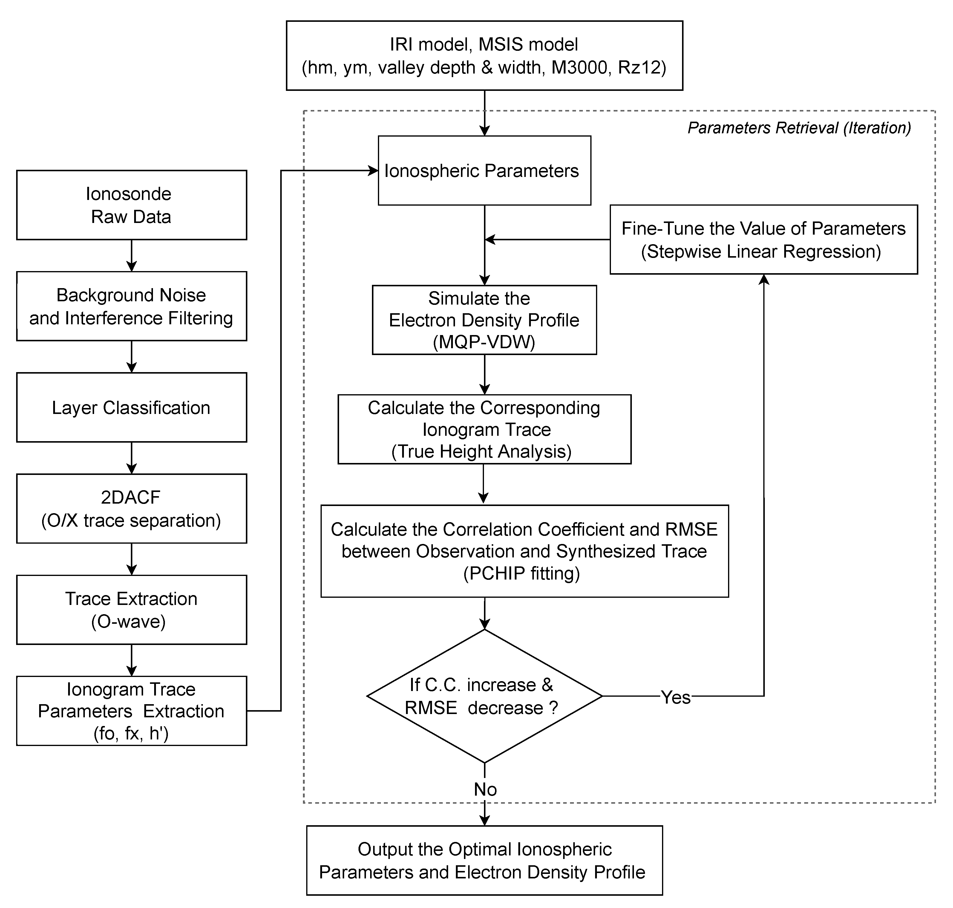
3. Autoscaling Algorithm

The data collected from the output of the ionosonde receiver can be properly arranged to generate an ionogram that displays the traces of the ordinary waves (O-waves) and extraordinary waves (X-waves) reflected from different layers of the ionosphere as a function of virtual height and frequency. Irrespective of the fact that the traces are very diverse, a well-trained and experienced operator can identify and scale the traces in the ionogram by the naked eye, provided that the ionogram is not significantly interfered with and the SNR of the traces is high enough. However, practically, it is not easy to design an algorithm that can automatically scale the ionogram to discern and extract the O-/X-wave traces for estimating ionospheric parameters through true height analysis, especially in the presence of radio frequency interference (RFI), clutters, and intense background noise in the ionogram. In this section, the autoscaling algorithm implemented in the Chung-Li ionosonde to retrieve the ionospheric electron density profile from the observed ionogram will be introduced, in which the processes of background noise and interference filtering, identification and extraction of the traces the of O- and X waves, quasi-parabolic segment model for ionospheric electron density profile, machine learning classification model, and stepwise linear regression procedure for true height analysis are included. A flowchart of the autoscaling algorithm is shown in Figure 4, and the details of each process will be described below.

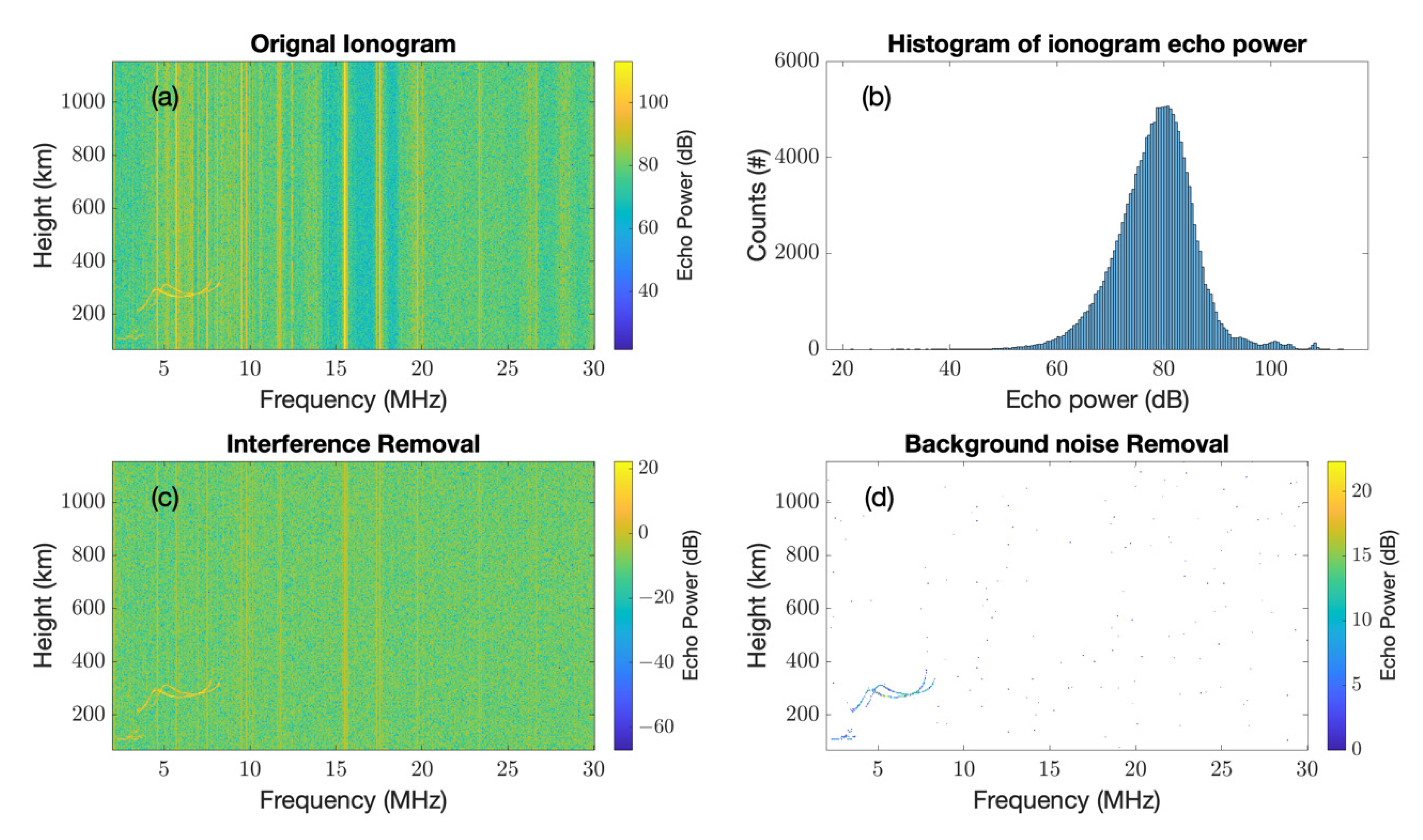
3.1. Background Noise and Interference Filtering Processing

In this study, we used statistical methods to remove the background noise and radio interference in the ionogram. Figure 5 shows the procedures of the statistical method. Figure 5a is a typical ionogram observed by the Chung-Li ionosonde, in which ionospheric traces, background noise, and intense radio interferences occurring at specific frequencies are present. Figure 5b shows a histogram of the echo intensity presented in Figure 5a. A comparison of Figure 5a,b indicates that the tail of the histogram distribution of the echo intensity with values larger than about 90 dB is dominated by ionospheric traces and intense radio interferences, and those with intensities less than 90 dB are background noise. In order to remove the interferences and underscore the traces, we calculated the mean value μ i and standard deviation σ i of the echo intensity at every frequency. We then subtracted the values of μ i + a i σ i from the original echo intensity at each frequency to produce the interference-removed ionogram, as shown in Figure 5c, where the value of a i was chosen to be 1.87. Notice that the echo power values shown in Figure 5c are relative to the value of 90 dB shown in Figure 5a. It is clear from Figure 5c that the interferences are significantly weakened and the traces are highlighted on the ionogram. With the same procedure of interference removal, we can underscore the traces further by subtracting the value of μ n + a n σ n from the echo intensity with interference removal, as shown in Figure 5c, where μ n and σ n are, respectively, the mean and standard deviation of the interference-removed echo intensity at every frequency, and the result is shown in Figure 5d.

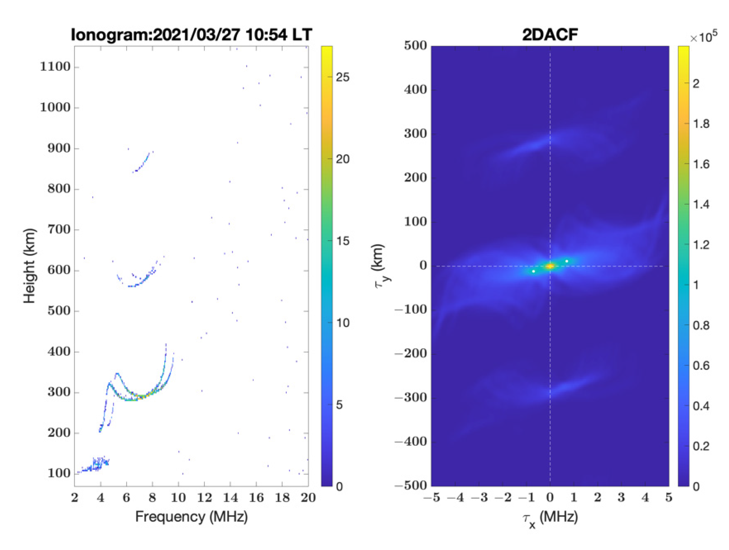
3.2. Two-Dimensional Autocorrelation

In light of the fact that only one receiving antenna with linear polarization is used in the Chung-Li ionosonde system to detect the radar returns from the ionosphere, an algorithm that can effectively discern and separate the traces of the O- and X-waves reflected from the F layer in the ionogram is required. In addition to wave polarization, the traces caused by multiple reflections of the echoes between the ionospheric layer and the ground should also be identified and removed to avoid errors in ionogram scaling. In this study, we used the two-dimensional autocorrelation function (2DACF) to identify the O- and X-waves and discern multiple reflection traces in the ionogram, which is defined below
AC ( τ x , τ y ) = i = m , j = n m , n F ( i , j )   F ( i + τ x , j + τ y )
where F ( i , j ) is the echo intensity at point (i, j) in the ionogram after the dilating process in this study, τ x   and   τ y   are, respectively, the displacements of the echo intensities along the x (frequency) and y (virtual height) axes, and m and n are, respectively, the numbers of total displacements of the frequency and virtual height. Figure 6 shows an example of 2DACF for the data recorded by the ionosonde on 27 March 2021, at 10:57 LT. As indicated, there are three peaks in the 2DACF. One major peak is located at τ x = 0   and   τ y = 0 , and two minor peaks are situated at τ x = Δ f e   and   τ y = Δ f O X , and τ x = Δ f e   and   τ y = Δ f O X , where the values of Δ f e and Δ f O X are, respectively, 0.7 MHz and 20 km. According to the magneto-ionic theory [1], the separation between the critical frequencies of the O- and X-waves is about half of the free electron gyrofrequency. Moreover, there is a small discrepancy in the reflection heights between O- and X-waves. Therefore, the distances of the minor peaks from the central major peak of the 2DACF carry the information of the free-electron gyrofrequency and virtual height difference between the O- and X-waves at the reflection height. In order to separate and extract the traces of the O- and X-waves, we first duplicated the ionogram and displaced the traces along the frequency axis by an amount of Δ f e . We then subtracted the displaced traces from the original traces. As a result, under the assumption that the O-wave traces bore high resemblance with the X-wave trace in pattern, the X-wave traces will be eliminated and only O-wave traces can be retained, and the parameters foF2 and h’F2 can thus be obtained. In an analogous manner, the X-wave traces can be acquired as well. Because of their relatively weak intensity, the traces of the E and F1 layers are not easy to identify and scale using the 2DACF method. We therefore used the projection method to identify and scale foF1 and foE in this study [13,14]. Additionally, in the presence of second-order reflection (or ground-reflected) traces in the ionogram, more 2DACF peaks are expected to occur at τ x = 0   and   τ y = Δ h and τ x = 0   and   τ y = Δ h , where Δh is the true virtual height of the original first-order reflection traces. Once the minor peaks of 2DACF are present and discerned, the second-order reflection traces can then be identified and removed from the ionogram. Figure 7 shows the scatter plot of the foF2 values obtained by the 2DACF method versus those obtained by the projection method. It is clear to see that the majority of the foF2 values determined by these two methods are very consistent with each other. Nevertheless, the projection method tended to generate more outliers with values larger than those determined by the 2DACF method, leading to a significant deviation from the line with a slope of 1 in the scatter plot.

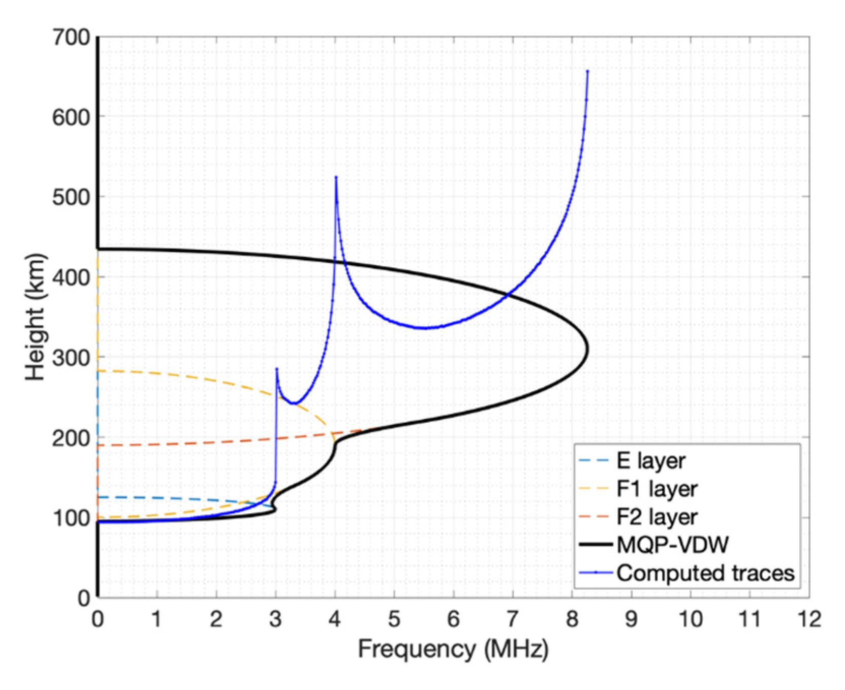
3.3. Ionospheric Modeling

Once the traces of the O- and X-waves are separated, we then carried out true height analysis to retrieve the ionospheric electron density profile. In this study, we used the quasi-parabolic segment (QPS) model to describe the electron density profile of ionospheric sublayers, namely, E, F1, and F2 layers [14,16]. The mathematical equation of a QP layer is defined below
{ f N 2 = f m 2 b ( 1 r m r ) 2 ,     r b < r < r m ( r b r b y m ) 0 ,     o t h e r w i s e
where f N is the plasma frequency, r is radial distance of the radar site from the Earth’s center, f m is the maximum plasma frequency at peak height r m with respect to the Earth’s center, r b = r m y m is the QP layer base height where the electron density is zero, y m is the semi-thickness of the layer, and b = r b 2 ( f m y m ) 2 . Note that if the multiple quasi-parabolic layer (MQP) model is employed to describe the height variation of ionospheric electron density that consists of E, F1, and F2 sublayers, the electron density at the intersection between the E and F1 sublayers and that between the F1 and F2 sublayers will be unrealistically discontinuous. In order to improve this problem, the multi-quasi-parabolic model with valley depth and width (MQP-VDW) model that was proposed by Sun et al. [17] will be adopted in this study. In the MQP-VDW model, a joint layer joins two QP sublayers above and below to provide a smoothed and continuous electron density profile in between, which is described by a QP curve similar to Equation (2) with an opening in the opposite direction to that of the QP sublayers. In this context, the following conditions should be fulfilled when describing the ionospheric electron density profile based on the MQP-VDW model
{ f J 2 | r = r M = f F 2 | r = r M f J 2 r | r = r M = f F 2 r | r = r M
where f J and f F are, respectively, the plasma frequencies of the joint layer and QP sublayer, and r M is the height of the intersection of the joint layer and QP sublayer. From Equations (2) and (3), after mathematical manipulation, the following relations are obtained
r M = b J r m J 2 + b F r m F 2 b J r m J + b F r m F
b J = ( a F a J ) b F r m F 2 a F r m J 2 a J r m J 2 b F r m J 2 b F r m F 2 + 2 b F r m F r m J
where r m J and r m F are, respectively, the plasma frequencies of the joint layer and QP sublayer at the respective vertexes, and b J and b F are the respective b values of the joint layer and QP sublayer in accordance with Equation (2). As a result, a continuous and smoothed profile of ionospheric electron density can be constructed.

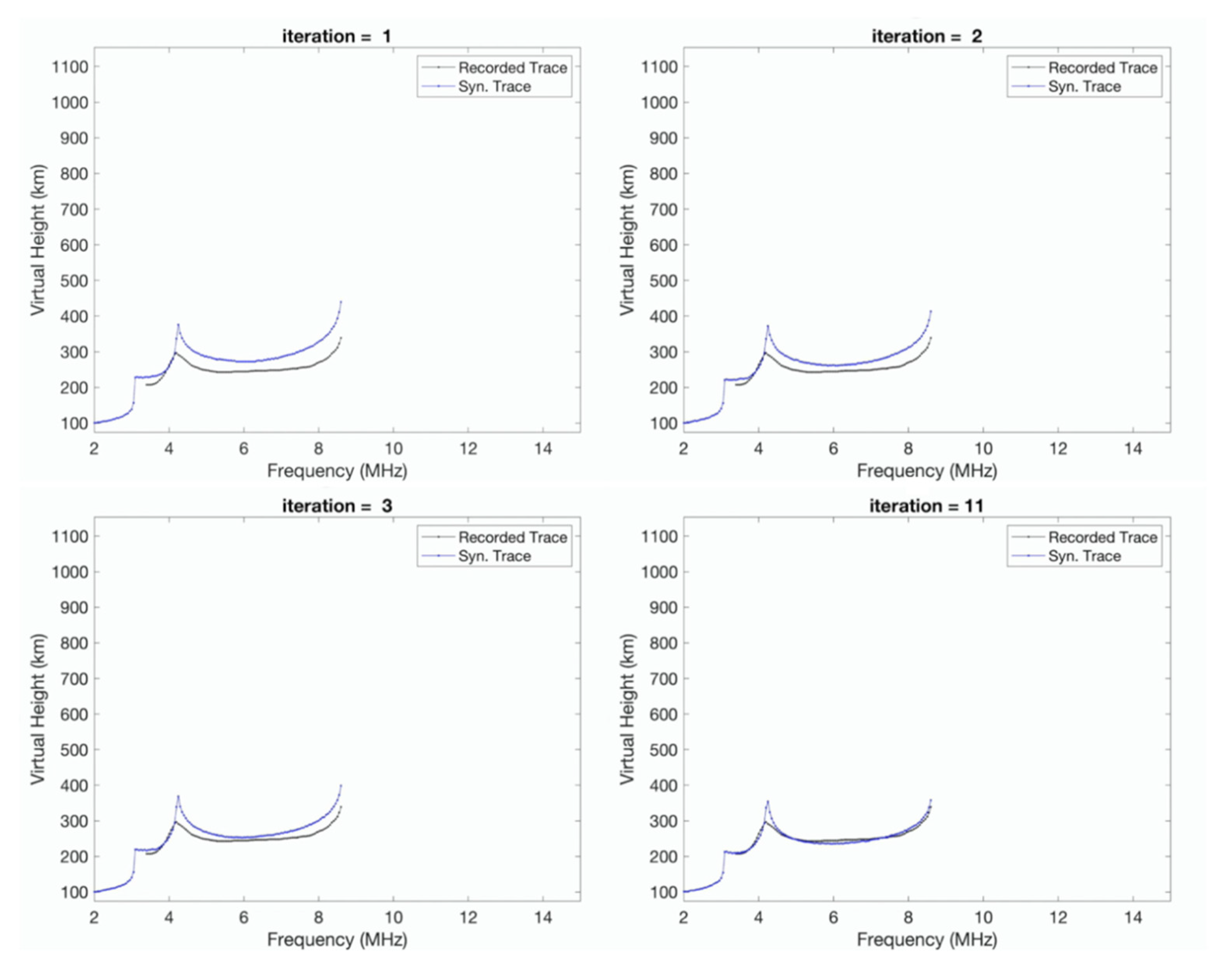
3.4. True Height Analysis

As indicated in (2)–(5), there are 11 ionospheric parameters required for the MQP-VDW model to construct an entire electron density profile of the bottom side of the ionosphere, namely, foE, hmE, ymE, foF1, hmF1, ymF1, foF2, hmF2, ymF2, D, and W, where D and W are, respectively, the parameters determined for the values of the depth foV(=foExD) and width hmV(=hmE + W/2) of the valley between the E and F1 layers. It is obvious that, at most, only three true ionospheric parameters (i.e., foF2, foF1, and foE) can be directly obtained through the scaling of the observed traces in the ionogram. In this study, the other eight parameters were borrowed from the IRI model to serve as the initial guesses for the true height analysis. Once the initial electron density profile N(h) that is constructed from the observed and modeled parameters is acquired, the virtual height h c of the corresponding trace can be computed in accordance with the following equation
h c = 0 h r 1 n p ( h ) d h i = 1 s 1 1 N m ( h i ) e 2 4 π 2 ε 0 m f 2 Δ h
where h r is the true reflection height, S is the number of height subintervals divided between 0 and h r , N m ( h i ) is the modeled electron density at the ith height subinterval, ε 0 (=8.85 × 10⁻¹² F m−1) is the permittivity of free space, m (=9.11 × 10⁻³¹ kg) is the electron mass, and e (=1.602 × 10⁻¹⁹ C) is the electron charge. Note that Δh is the height resolution, which is a function of the phase refractive index of the ionosphere n p ( h ) to mitigate the divergence problem of integration in the context of n p ( h ) 0 [9]. Figure 8 shows an example of the modeled electron density profile N m ( h ) with the MQP-VDW model and corresponding ionogram traces that were computed in accordance with Equation (6), in which the dashed curves with different colors represent the modeled electron density profiles of the respective ionospheric sublayers, the black curve is the integrated electron density profile from the MQP-VDW model with three QP layers and the valley within E and F layer, and the blue curves with dots are the computed traces of the modeled electron density profiles. Obviously, the computed virtual height h c in accordance with Equation (6) with a modeled electron density profile will bear a discrepancy from the observed virtual height h o that corresponds to a real electron density profile N r ( h ) . In this study, on the basis of the fine-tuned model that was established through stepwise regression analysis of the IRI model data and the difference Δ h between h o and h c , we could gradually adjust the values of the ionospheric parameters that were the inputs of the MQP-VDW model to reduce Δ h . The independent variables that we used for the stepwise regression analysis in this study included Δ h , mean Δ h ( Δ h ¯ ), and the values of α and β that were, respectively, the intercept and slope of the linear regression line between Δ h and f, namely, Δ h = α + β f . Note that stepwise regression analysis is a systematic method to add or remove the terms in a multilinear regression model based on their statistical significance in the regression analysis. According to the thresholds that we set in the true height analysis, the optimal ionospheric parameters could eventually be achieved as the root mean squared error (RMSE) between h o and h c is minimum and their correlation coefficient (c.c.) is high enough, and both of them meet the preset thresholds. As a result, the corresponding modeled N m ( h ) can be regarded to come very close to the real N r ( h ) and accepted as the output of the true height analysis.
Figure 9 is an example showing the steps of the model-simulated traces (blue curve) that gradually approach the observed traces (black curve) by adjusting the ionospheric parameters for the MQP-DVW model through stepwise regression analysis. Once the values of the RMSE and correlation coefficient between h o and h c both reach the respective thresholds, the step of the iteration will stop to complete the true height analysis, and the final N m ( h ) is adopted as the true electron density profile. Figure 10 shows an example of the result of true height analysis. As indicated, irrespective of the presence of intense radio frequency interference in the original ionogram (top panel), the autoscaling algorithm can still identify and separate the traces of O-waves (red curve) and X-waves (blue curve), and the electron density profile shown in the bottom panel can also be retrieved by using the stepwise regression analysis. Note that the top-side electron density profile was constructed in accordance with the IRI model, which follows an exponential profile, rather than the QPS model. The total time that was needed to process the raw radar echoes and perform autoscaling of the ionogram to produce the resultant electron density profile was 294.13 s, as shown in Table 1.

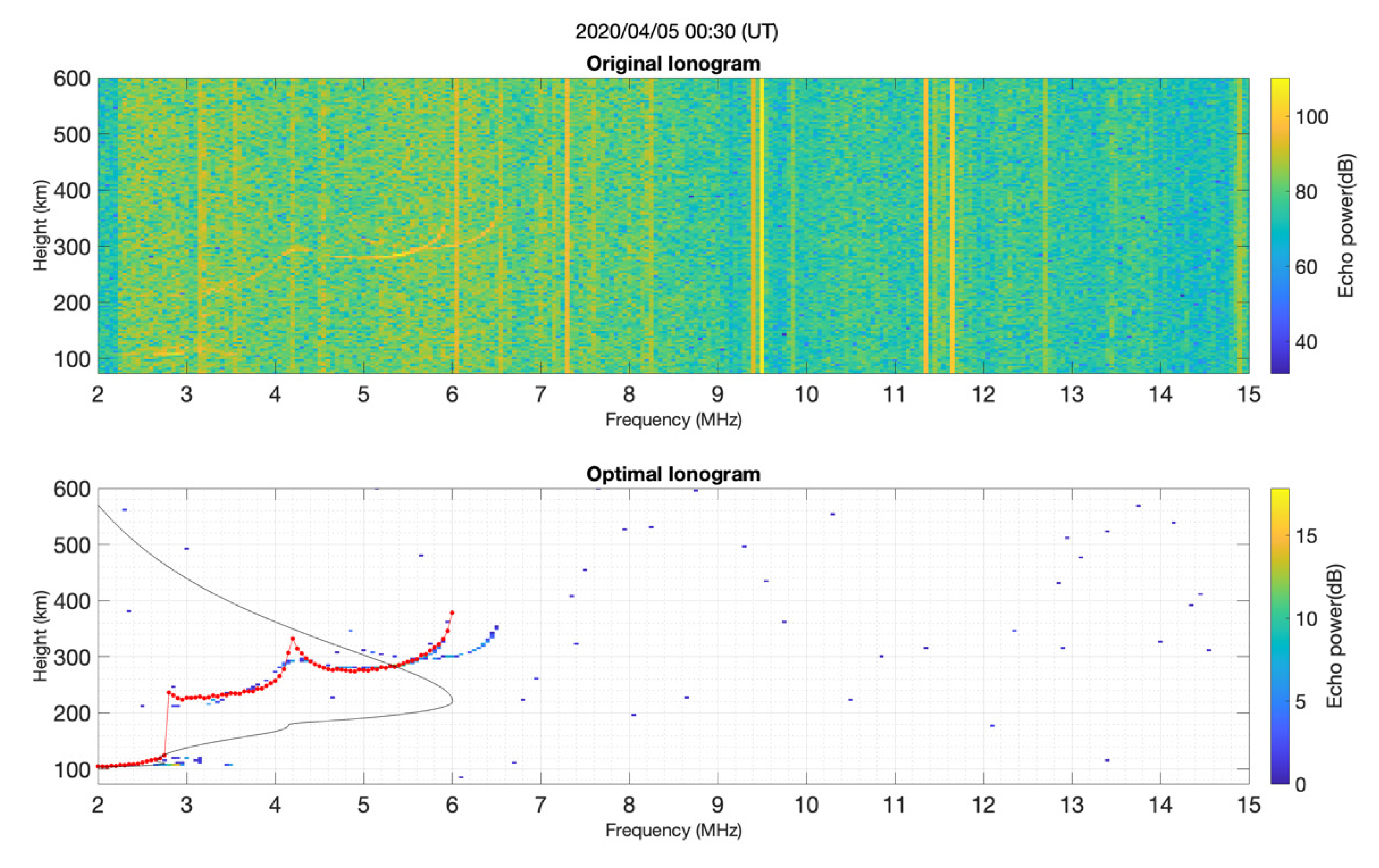
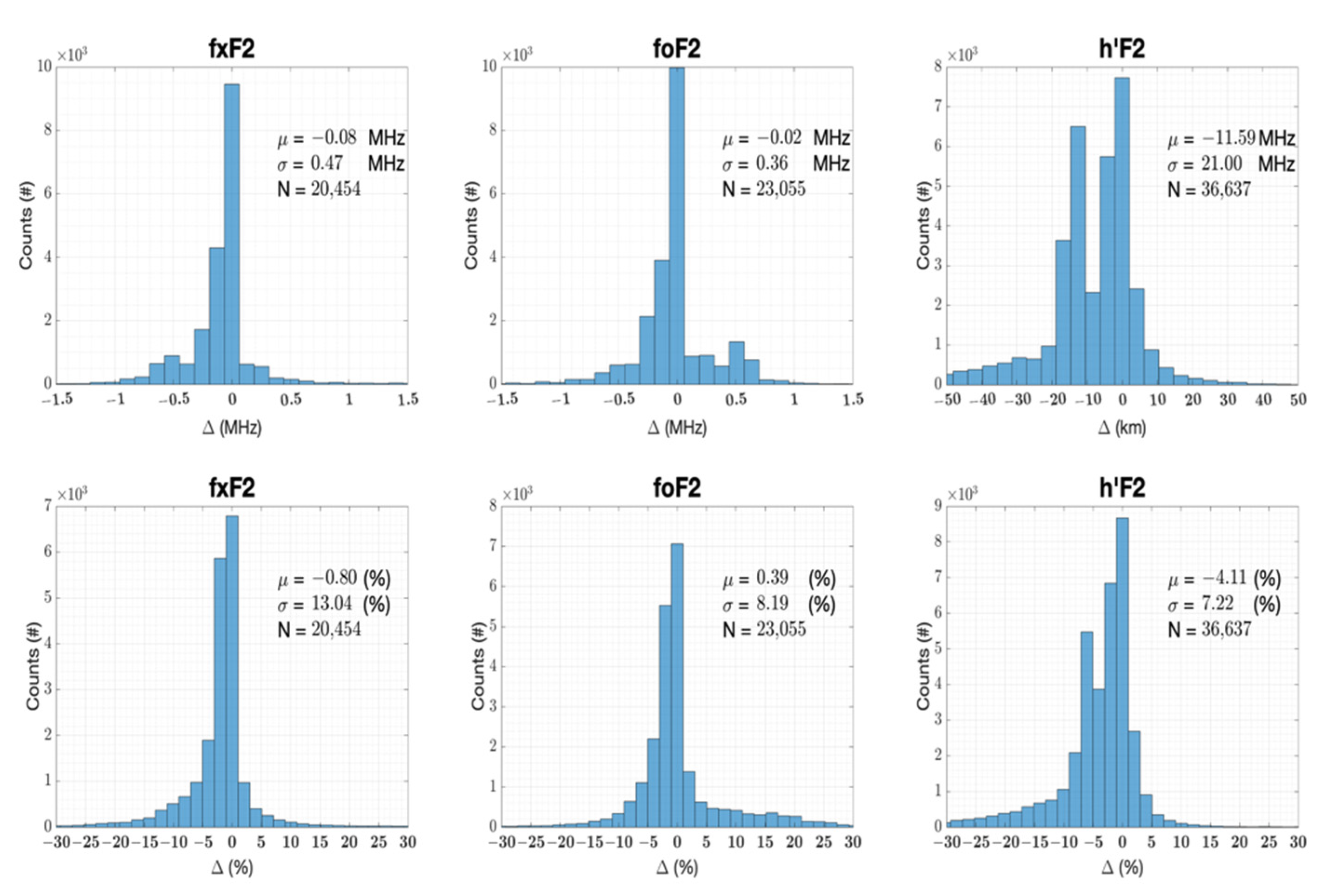
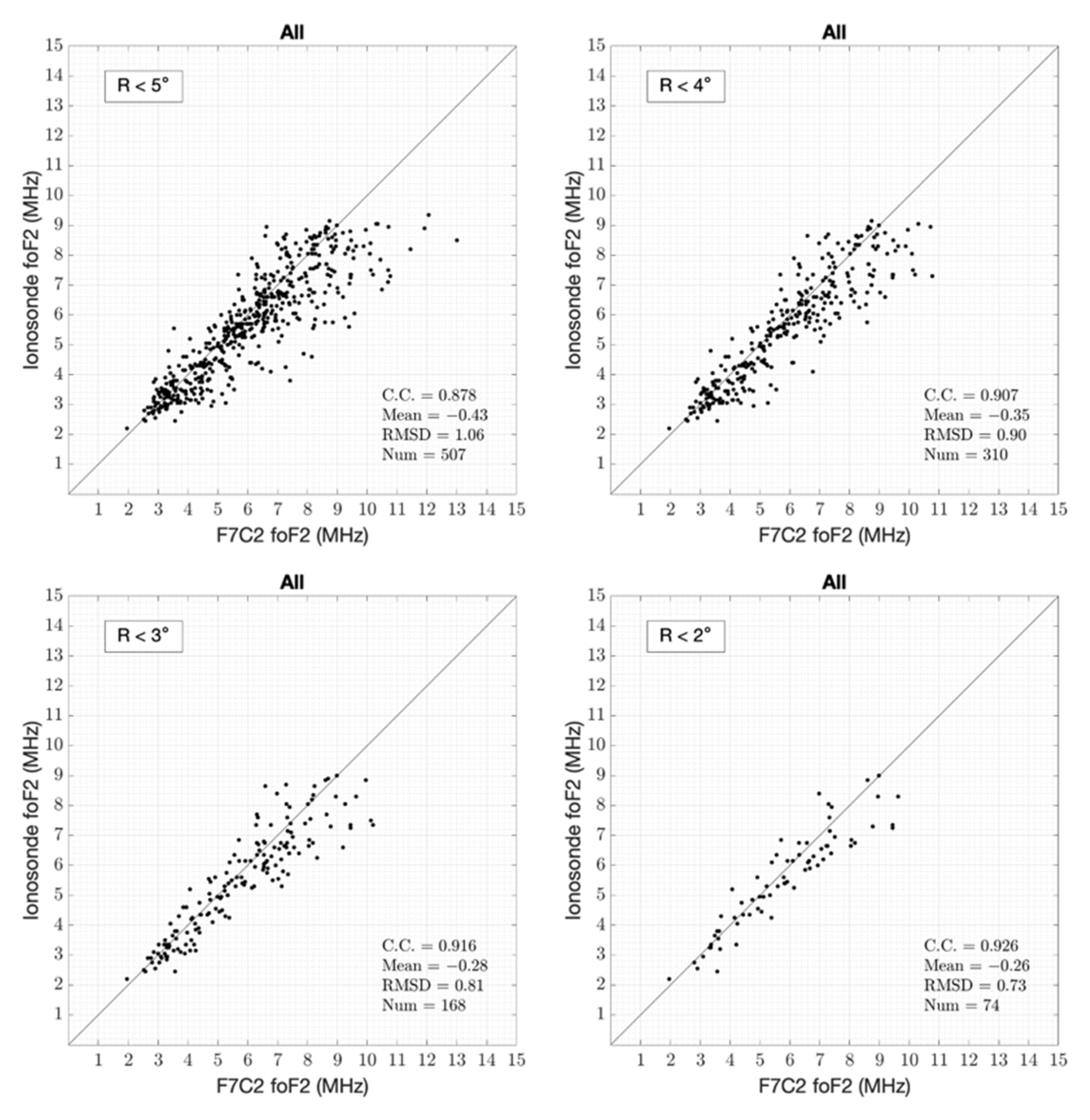
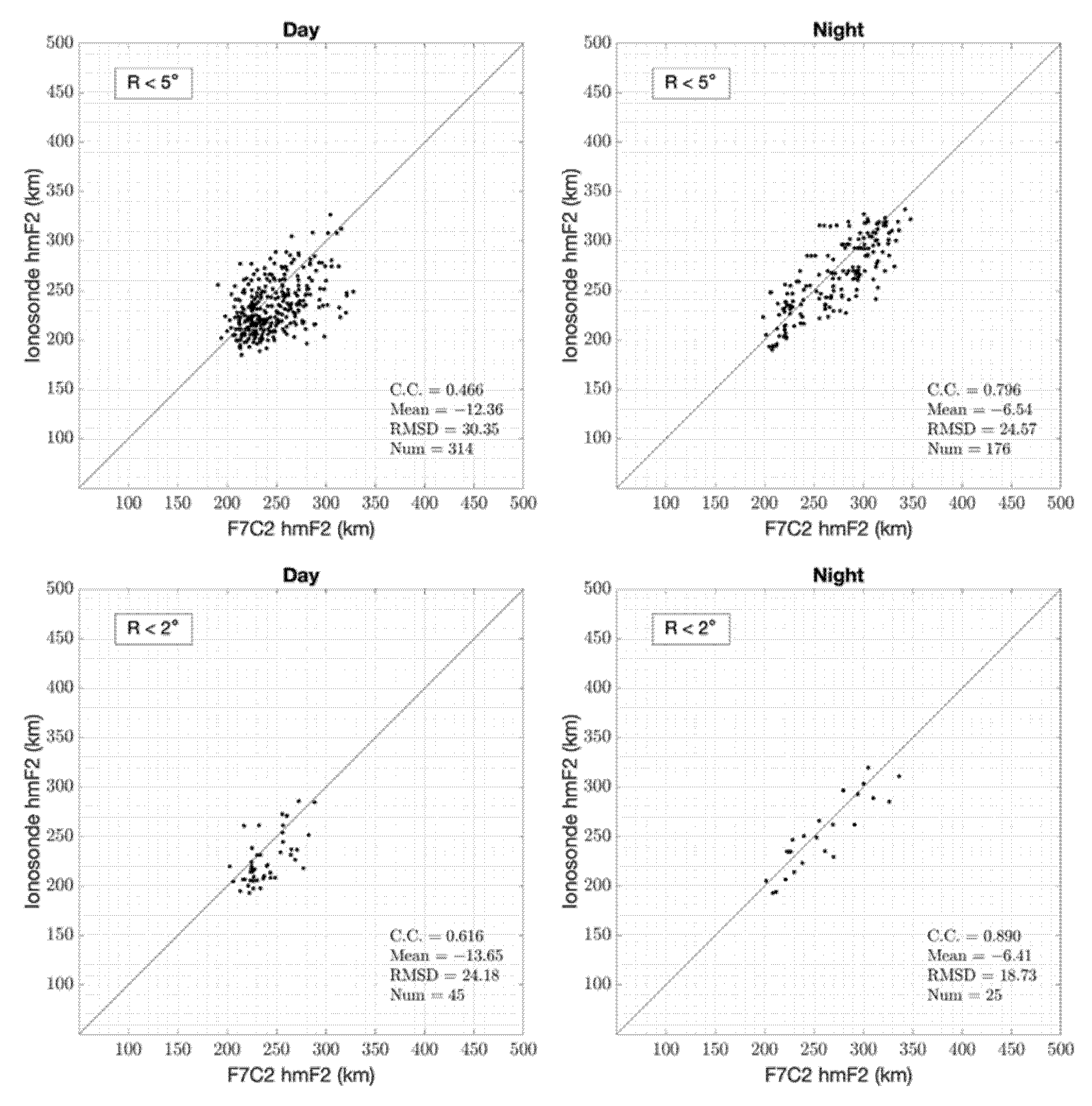
4. Preliminary Results

In order to validate the autoscaling algorithm developed in this study for the Chung-Li ionosonde, we first compared the values of foF2 and h’F2 obtained from the autoscaling algorithm and manual scaling for the period from 1 April 2020 to 24 March 2021. The upper panels of Figure 11 display the histograms of the differences in fxF2 (left), foF2 (middle), and h’F2 (right) between autoscaling and manual scaling for April 2020–March 2021. As shown, the means and the standard deviations of the differences (autoscaling minus manual scaling) in fxF2, foF2, and h’F2 were, respectively, −0.1 and 0.41 MHz, 0 and 0.36 MHz, and −0.06 and 15.36 km. The lower panels of Figure 11 show the percentage differences (PDs) of fxF2, foF2, and h’F2, which are defined as follows.
PD ( % ) = a u t o m a n u a l m a n u a l × 100
As shown, the means and the standard deviations of PD in fxF2, foF2, and h’F2 were, respectively, −1.43% and 10.56%, 0.84% and 8.09%, and 0.06% and 5.67%. These results signify that the fxF2, foF2, and h’F2 obtained from the autoscaling algorithm were reliable and consistent with those from manual scaling.
In addition to analyzing the consistency in the foF2 and h’F2 between autoscaling and manual scaling, we also compared the values of foF2 and hmF2 between the ionosonde measurement and the GPS RO retrieval made with the FORMOSAT-7 (or COSMIC2) satellites for the period from 1 April 2020 to 24 March 2021. Figure 12 displays scatter diagrams of the ionosonde-measured foF2 (ionosonde-foF2) versus the GPS RO-retrieved foF2 (F7C2-foF2) for various spatial coverages, in which R is the radius of the spatial coverage centered at the Chung-Li ionosonde station, where F7C2-foF2 was collected to compare with ionosonde foF2. As shown, the ionosonde foF2 values were, in general, consistent with F7C2-foF2. The correlation coefficient (c.c.), the root mean squared deviation (RMSD), and mean difference between them were, respectively, in ranges from 0.878 to 0.926, 0.73 to 1.06 MHz, and −0.43 to −0.26 MHz. With the decrease in R, the correlation coefficients tended to become high, and their mean difference and the RMSD tended to be both small. Figure 13 shows comparisons of the peak electron density heights between the ionosonde measurements (ionosonde-hmF2) and FORMOSAT-7 retrievals (F7C2-hmF2) for different spatial coverages. As indicated, the correlation coefficient (c.c.), the root mean squared deviation (RMSD), and the mean difference between them were, respectively, in ranges from 0.701 to 0.797, 22.39 to 28.45 km, and −9.28 to 11.06 km.

5. Discussion

From Figure 12 and Figure 13, we can observe that the larger the radius R is, the more scattered the data points are, and the smaller (larger) the correlation coefficient (RMSE) will be. This feature suggests that the spatial separation of the data sampling locations between the ionosonde and the GPS RO sounding is one of the dominant factors affecting the performances of the data comparisons of foF2 and hmF2. In addition, a detailed examination of the scatter distributions of the foF2 values shown in Figure 12 indicated that F7C2-foF2 with values greater than 4 MHz was the primary cause of the large mean difference and the RMSD, especially for those in the data-collecting region with R > 3°. In order to realize the plausible cause of this abnormally large F7C2-foF2, Figure 14 compares the scatter plots of ionosonde foF2 versus F7C2-foF2 during the daytime (from 8 to 20 LT) (left panels) and nighttime (from 20 to 8 LT) (right panels) for sampling radii of 5° (upper) and 2° (lower) of the FORMOSAT-7 data. It is clear that the data points with abnormally large F7C2-foF2 values that significantly deviated from the line with a slope of 1 occurred mainly during the daytime and occurred less frequently or very little during the nighttime, especially for those in the sampling region with R < 2°. In light of the fact that the ionospheric peak electron densities during the daytime were substantially larger than those during the nighttime, the abnormally large F7C2-foF2 values above 4 MHz were very likely the result of the spatial separation combined with the daytime ionization. Consequently, the RMSE and mean difference values for the foF2 data during the nighttime were much smaller than those during the daytime, as shown in Table 2. Figure 15 shows the scatter diagrams of ionosonde-hmF2 versus F7C2-hmF2 collected during the daytime (left panels) and nighttime (right panels) for sampling radii of 5° (upper) and 2° (lower) of the FORMOSAT-7 data. As indicated, the mean difference between ionosonde-hmF2 and F7C2- hmF2 during the nighttime, either for R < 2° or R < 5°, was substantially smaller than that that during the daytime by a factor of 2. In addition, the majority of the data points were distributed along the line of slope 1, especially for the data during the nighttime. This result suggests the consistency of the hmF2 values between the ionosonde measurements and the GPS RO retrievals. Table 3 summarizes the comparisons of the correlation coefficients (c.c.), RMSDs, and mean differences between the ionosonde-measured hmF2 and F7C2-hmF2.
Chu et al. [18] compared global foF2 data measured by ground-based ionosondes and those retrieved by FORMOSAT-3 satellites using the GPS RO technique and showed that there is a tendency for the ionosonde-measured peak electron densities (or foF2) in the equatorial ionospheric region (EIA) region to be smaller than those retrieved by FORMOSAT-3 satellites. Hu et al. [19] analyzed the latitudinal variations in the ionosonde NmF2 data and COSMIC-2 NmF2 data collected over mainland China in a longitudinal zone from about 109°E to 122°E and showed that, during the daytime, the COSMIC-retrieved NmF2 significantly exceeded the ionosonde-measured NmF2 by about 38.9% on average at Wuhan station (geographic latitude 31.0°N and geomagnetic latitude 20.8°), which is located in the EIA region, while, during the nighttime, they were in excellent agreement with each other, with a very small RMSE. The simulation study carried out by Shaikh et al. [20] indicated that the presence of a horizontal electron density gradient in the occultation plane can lead to retrieval error in the electron density profile at the tangent point of the GPS ray due to the violation of the spherical symmetry assumption required in retrieving the electron density profile based on Abel transformation. Note that the Chung-Li ionosonde is situated in the crest zone of the EIA region that is characterized by a profoundly large horizontal electron density gradient. Our results presented in Figure 12 and Figure 14 are very consistent with others’ results [18,19,20]. Therefore, this suggests that the overestimation of the COSMIC-retrieved foF2 during the daytime is the result of a GPS RO retrieval error caused by the horizontal gradient of the electron density in the occultation plane.

6. Conclusions

In this article, the system configuration and the autoscaling algorithm of the new Chung-Li ionosonde are introduced, which was started to be constructed in 2018 and routinely operated in April 2020. We present the system layout of the ionosonde, including the TX/RX systems, antenna configuration and antenna pattern, radar signal processing, time synchronization, and so on. In addition, the algorithms of trace scaling and true height analysis are also deliberated. On the basis of the 2-dimensional autocorrelation function (2DACF) combined with the image-projection method, we developed a new autoscaling algorithm to process the ionogram data to identify and separate the O- and X-waves of the traces. The MQP-VDW model was employed to describe the electron density profile for true height analysis. Stepwise regression analysis was performed to adjust the ionospheric parameters for the input of the MQP-VDW model to retrieve the true electron density profile. We found that the 2DACF method was superior to the image-projection method in the performance of the identification of O-wave for the determination of foF2, in which the uncertainty of the foF2 values determined by the former was smaller than those by the latter. We also compared the foF2 and hmF2 values observed by the new Chung-Li ionosonde and those retrieved by the FORMOSAT-7 satellites by using the GPS RO technique to validate the capability of observing the ionospheric parameters made by the new Chung-Li ionosonde. We found that, with the decrease in the radius of spatial coverage selected for ionospheric parameter comparison between the Chung-Li ionosonde and FORMOSAT-7 satellites, the correlation coefficients tended to become high, and the mean difference and the RMSD tended to both be small. For a radius smaller than 2°, the corresponding correlation coefficient, root mean squared deviation, and mean difference were, respectively, 0.93, 0.73, and −0.26 MHz for foF2 and 0.8, 22.39, and −11.06 km for hmF2. These results show that, regardless of the minor mismatches of the limited data points caused by the GPS RO retrieval error, the ionosonde measurements are essentially consistent with the FORMOSAT-7 retrievals.

Author Contributions

Conceptualization, Y.-H.C., C.-L.S. and K.-J.K.; Methodology, Y.-H.C., K.-J.K.; Formal Analysis, Y.-H.C., C.-L.S. and K.-J.K.; Validation, Y.-H.C., K.-J.K., H.-S.L., P.-H.C. and C.-Y.K.; Investigation, Y.-H.C. and K.-J.K.; Ionosonde Installation and System Integration, C.-L.S., R.-M.K. and H.-C.C.; Data Curation, C.-L.S.; Writing—Original Draft Preparation, K.-J.K. and R.-M.K.; Writing—Review and Editing, Y.-H.C. and C.-L.S.; Supervision, Y.-H.C. and C.-L.S.; Funding Acquisition, Y.-H.C. and C.-L.S. All authors have read and agreed to the published version of the manuscript.

Funding

This research received no external funding.

Institutional Review Board Statement

Not applicable.

Informed Consent Statement

Not applicable.

Data Availability Statement

The data that were employed to support the findings of this study belong to CWB and are available from the corresponding author upon request.

Acknowledgments

This work was financially supported by the Central Weather Bureau (CWB), Ministry of Transportation in Taiwan, under contract #1062302D.

Conflicts of Interest

The authors declare that they have no competing interest.

References

  1. Davies, K. Ionospheric Radio Wave Propagation; P. Peregrinus on behalf of the Institution of Electrical Engineers: London, UK, 1989. [Google Scholar]
  2. Reinisch, B.W.; Huang, X. Automatic calculation of electron density profiles from digital ionograms: 3. Processing of bottomside ionograms. Radio Sci. 1983, 18, 477–492. [Google Scholar] [CrossRef]
  3. Galkin, I.A.; Reinisch, B.W.; Ososkov, G.A.; Zaznobina, E.G.; Neshyba, S.P. Feedback neural networks for artist ionogram processing. Radio Sci. 1996, 31, 1119–1128. [Google Scholar] [CrossRef]
  4. Pezzopane, M.; Scotto, C. The INGV software for the automatic scaling of foF2 and MUF(3000)F2 from ionograms: A comparison with ARTIST 4.01 from Rome data. J. Atmos. Sol.-Terr. Phys. 2005, 67, 1063–1073. [Google Scholar] [CrossRef]
  5. Galkin, I.A.; Reinisch, B.W. The New ARTIST 5 for All Digisondes; University of Massachusetts Lowell Center for Atmospheric Research: Lowell, MA, USA, 2008. [Google Scholar]
  6. Zabotin, N.A.; Wright, J.W.; Zhbankov, G.A. NeXtYZ: Three-dimensional electron density inversion for dynasonde ionograms. Radio Sci. 2006, 41. [Google Scholar] [CrossRef] [Green Version]
  7. Pezzopane, M.; Scotto, C. A method for automatic scaling of F1 critical frequencies from ionograms. Radio Sci. 2008, 43. [Google Scholar] [CrossRef] [Green Version]
  8. Scotto, C.; Pezzopane, M. A Software for Automatic Scaling of foF2 and MUF(3000) F2 From Ionograms. 2002, pp. 17–24. Available online: http://old.ursi.org/proceedings/procGA02/papers/p1018.pdf (accessed on 1 March 2022).
  9. Scotto, C.; Pezzopane, M.; Zolesi, B. Estimating the vertical electron density profile from an ionogram: On the passage from true to virtual heights via the target function method. Radio Sci. 2012, 47. [Google Scholar] [CrossRef]
  10. Tsai, L.C.; Barkey, F.T. Ionogram analysis of ionograms: A generalized formulation. Radio Sci. 2000, 35, 1173–1186. [Google Scholar] [CrossRef] [Green Version]
  11. Pillat, V.; Guimarães, L.; Fagundes, P.; Silva, J. A computational tool for ionosonde CADI’s ionogram analysis. Comput. Geosci. 2013, 52, 372–378. [Google Scholar] [CrossRef]
  12. Ding, Z.-H.; Ning, B.-Q.; Wan, W.-X. Real-time automatic scaling and analysis of ionospheric ionogram parameters. Chin. J. Geophys. 2007, 50, 837–847. [Google Scholar] [CrossRef]
  13. Jiang, C.H.; Yang, G.B.; Zhao, Z.Y.; Zhang, Y.N.; Zhu, P.; Sun, H.Q. An automatic scaling technique for obtaining F2 parameters and F1 critical frequency from vertical incidence ionograms. Radio Sci. 2013, 48, 739–751. [Google Scholar] [CrossRef]
  14. Jiang, C.H.; Yang, G.B.; Zhao, Z.Y.; Zhang, Y.N.; Zhu, P.; Sun, H.Q.; Zhou, C. A method for the automatic calculation of electron density profiles from vertical incidence ionograms. J. Atmos. Sol.-Terr. Phys. 2014, 107, 20–29. [Google Scholar] [CrossRef]
  15. Jiang, C.H.; Yang, G.B.; Lan, T.C.; Zhu, P.; Song, H.; Zhou, C.; Cui, X.; Zhao, Z.Y.; Zhang, Y.N. Improvement of automatic scaling of vertical incidence ionograms by simulated annealing. J. Atmos. Sol.-Terr. Phys. 2015, 133, 178–184. [Google Scholar] [CrossRef]
  16. Norman, R.J. An Inversion Technique for obtaining Quasi-Parabolic layer parameters from VI Ionogram. In Proceedings of the 2003 International Conference on Radar, Adelaide, Australia, 3–5 September 2003. [Google Scholar]
  17. Sun, J.X.; Zhang, J.; Wang, S.; Gong, Z.Q.; Fang, G.Y. Multi-quasi-parabolic ionosphere model with EF-valley. Ann. Geophys. 2016, 59, A0213. [Google Scholar] [CrossRef]
  18. Chu, Y.-H.; Su, C.-L.; Ko, H.-T. A global survey of COSMIC ionospheric peak electron density and its height: A comparison with ground-based ionosonde measurements. Adv. Space Res. 2010, 4, 431–439. [Google Scholar] [CrossRef]
  19. Hu, L.; Ning, B.; Liu, L.; Zhao, B.; Li, G.; Wu, B.; Huang, Z.; Hao, X.; Chang, S.; Wu, Z. Validation of COSMIC ionospheric peak parameters by the measurements of an ionosonde chain in China. Ann. Geophys. 2014, 32, 1311–1319. [Google Scholar] [CrossRef] [Green Version]
  20. Shaikh, M.M.; Notarpietro, R.; Nava, B. The impact of spherical symmetry assumption on radio occultation data inversion in the ionosphere: An assessment study. Adv. Space Res. 2014, 53, 599–608. [Google Scholar] [CrossRef]
Figure 1. Block diagram of the radar system of the Chung-Li ionosonde, in which the major functional units of the radar system and the primary interconnections between the units are shown. For the details of the units, refer to the text.
Remotesensing 14 01913 g001
Figure 2. Drawing of the 54 m-long three-wire inverted-V dipole antenna of the Chung-Li ionosonde, in which the 2 m fiberglass post on top of the 13 m pole is highlighted.
Remotesensing 14 01913 g002
Figure 3. Three-dimensional radiation patterns of the inverted V dipole antenna for different operating frequencies, in which the 3D radiation patterns at frequencies of 2, 7, 10, 15, 20, and 30 MHz are shown.
Remotesensing 14 01913 g003
Figure 4. Flowchart of the autoscaling algorithm in this study; the outputs of the algorithm are the optimal ionospheric parameters and corresponding electron density profile.
Remotesensing 14 01913 g004
Figure 5. Processes of removing background noise and interference in the ionogram for extracting traces. (a) Original ionogram; (b) echo power histogram of the original ionogram; (c) interference-removed ionogram; (d) background noise-removed ionogram, in which the traces are underscored.
Remotesensing 14 01913 g005
Figure 6. Example of the 2DACF (right) of the traces (left) in the ionogram. The contour represents the number of overlapped points, and τ x and τ y are, respectively, the horizontal (frequency) and vertical (virtual height) displacements of the traces. The yellow dot is the major peak of the 2DACF, and the two white dots on each side of the yellow dot mark the secondary minor peaks that resulted from the overlaps of the O- and X-wave traces. The horizontal separation between the major and minor peaks in frequency is equal to half of the electron gyrofrequency, which is about 0.7 MHz for the present case.
Remotesensing 14 01913 g006
Figure 7. Scatter diagram of foF2 estimated from the 2-dimensional autocorrelation function (2DACF) versus the projection method.
Remotesensing 14 01913 g007
Figure 8. An example showing simulated electron density profiles with the MQP-VDW model and corresponding ionogram traces from the true height analysis. The dashed curves with different colors represent the electron density profiles of the respective ionospheric sublayers based on the QP model. The black curves show the simulated electron density profile from the MQP-VDW model with three QP layers and the valley within the E and F layer. The blue curves with dots are the computed traces of the modeled electron density profiles.
Remotesensing 14 01913 g008
Figure 9. Examples showing the model-simulated ionogram traces that gradually approached the observed traces by adjusting the ionospheric parameters for the MQP-DVW model through stepwise regression analysis.
Remotesensing 14 01913 g009
Figure 10. (Top) Original ionogram recorded on 05 April 2020 at 00:30 UT by the Chung-Li ionosonde; (Bottom) identified O-wave (red curve), X-wave (blue curve), and the corresponding electron density profile (black curve) made with the autoscaling algorithm.
Remotesensing 14 01913 g010
Figure 11. Histograms of the differences (upper) and the percentage differences (lower) in fxF2, foF2, and h’F2 between autoscaling and manual scaling for the data collected from 1 April 2020 to 24 March 2021, in which the difference is the autoscaling minus manual scaling, and the percentage difference is defined as PD ( % ) = ( a u t o m a n u a l ) × 100 / m a n u a l .
Remotesensing 14 01913 g011
Figure 12. Scatter diagrams of manually scaled foF2 from the ionograms measured by the Chung-Li ionosonde versus FORMOSAT-7 retrieved foF2 using the GPS RO technique for the different spatial coverages with the radiuses centered at the Chung-Li ionosonde station.
Remotesensing 14 01913 g012
Figure 13. Same as Figure 12, but for hmF2.
Remotesensing 14 01913 g013
Figure 14. Daytime (left) and nighttime (right) scatter plots of the ionosonde foF2 versus F7C2 foF2 for radii of 5° (upper) and 2° (lower) for spatial coverage.
Remotesensing 14 01913 g014
Figure 15. Same as Figure 14, but for hmF2.
Remotesensing 14 01913 g015
Table 1. Characteristics of Chung-Li ionosonde.
ParametersValues
Frequency range (MHz)2–30
Frequency steps (kHz)50, 100
Pulse length (μs)166.4, 204. 8, 332. 8, 409.6
Pulse coding13-bit Barker code, or 16-bit Complementary Code, or single pulse
Chip width (μs)12.8, 25.6
Pulse waveformTrapezoid or Gaussian
Inter-pulse period (ms)4.096, 8.192
Pulse repetition frequency (Hz)122, 244
Number of pulses transmitted per frequency32
Maximum duty cycle (%)7.5
Height range (km)70–1221
Height resolution (km)1.92, 3.84
Peak pulse power (W)10–600
Ionogram process time (s)294.13
Table 2. Comparison of c.c., RMSD and mean difference ( d ¯ ) for foF2.
Radius (deg)c.c.RMSD (MHz) d ¯ (MHz)
AllDayNightAllDayNightAllDayNight
50.880.750.801.061.230.68−0.43−0.53−0.26
40.910.820.840.901.030.64−0.35−0.41−0.26
30.920.830.920.810.980.44−0.28−0.35−0.17
20.930.850.940.730.880.37−0.26−0.36−0.09
c.c.: Correlation Coefficient, RMSD: Root Mean Squared Deviation, d ¯ = [ f o F 2 ( i o n o s o n d e ) f o F 2 (COSMIC2)]/N.
Table 3. Comparison of c.c., RMSD and mean difference ( d ¯ ) for hmF2.
Radius (deg)c.c.RMSD (km) d ¯ (km)
AllDayNightAllDayNightAllDayNight
50.700.480.8028.4530.4024.63−10.66−12.93−6.63
40.760.550.8425.6427.5722.14−9.8−10.78−6.83
30.770.560.8724.6627.1319.84−10.16−12.35−6.48
20.800.620.8922.3924.1818.73−11.06−13.65−6.41
c.c.: Correlation Coefficient, RMSD: Root Mean Squared Deviation, d ¯ = [ h m F 2 ( i o n o s o n d e ) h m F 2 (COSMIC2)]/N.
Publisher’s Note: MDPI stays neutral with regard to jurisdictional claims in published maps and institutional affiliations.

