1. Introduction
Climate warming has increased the danger of wildfire disasters around the world. One of the most serious dangers to wildland ecosystems is fire. Fire is regarded as a key factor in both the growth and the degradation of wildland ecosystems globally [
1,
2]. Despite the fact that fire has always been a force in landscape modification and renewal, fire occurrences can have severe human, environmental, and economic repercussions, particularly when they become huge wildfires [
3]. They can have a deleterious impact on the composition and structure of fauna and flora, as well as the quality of air, soil, and water [
4,
5]. They also result in financial losses and endanger human health and life [
6,
7,
8,
9]. Increased fire frequency and intensity have been observed in Asian countries, albeit at varied rates. According to several studies, global climate change will likely increase the frequency and intensity of wildfires in most parts of the world in the future [
10,
11,
12,
13,
14]. Pakistan has one of the world’s lowest forest covers, with only 4.5% of its land covered in forest, and it is experiencing significant forest depletion [
15]. During the second half of the 20th century, there was evidence of higher fire incidence than prior years in Pakistan, as well as in other regions, a constant increase in the frequency of big wildfires, and an increase in the length of burned territory [
2,
16].
Wildfire hazard is defined as an assessment of the constant and dynamic characteristics that influence the ease of ignition, spread rate, control difficulty, and fire impact [
17]. The four decisive requirements for wildfire occurrence and spread, according to [
18], are favorable climatic circumstances, the presence of fuel, its spatial continuity, and a source of ignition. Weather factors, human behavior, vegetation traits, fuel availability, and topography are among the most essential [
19,
20]. The driving variables of wildfires are separated into three categories: (i) topography, (ii) climatic, and (iii) fuel; Each factor’s impact on the assessment of wildland fire risk varies depending on its geographical and temporal variability. The importance of climatic elements in the analysis of wildfire patterns has been shown by various studies [
21,
22]. Several researchers addressed the effect of different topographic features (slope, aspect, and height) on burned area and ignition density, although the importance and direction of this association varied across studies [
23]. Fuel is the most important factor in fire ignition and propagation, and varied vegetation patterns increase landscape fire susceptibility [
24,
25]. Despite the fact that many fires are ignited by humans, the main characteristics of local vegetation continue to be a determining factor in wildfire risk, as they determine the success of the ignition event and, more critically, fire behavior [
26]. Lastly, human factors are widely acknowledged as some of the primary causes of wildfires. Population density and dynamics, socioeconomic characteristics, changes in land cover, infrastructure, and human activities such as agriculture and livestock husbandry are all examples of fuel variables [
23,
27]. It is worth noting that, unlike nonhuman forces, human factors are largely nonstationary in time and place [
28,
29]. Due to enormous resource requirements, i.e., complexity, as well as varied data formats, modeling many complex environmental and socioeconomic independent variables is often a tough endeavor. Most predictor variables, such as temperature, precipitation, and population, are acquired from open-source satellite imagery in this regard. Satellite remote sensing has become a standard technique for large-scale ecosystem monitoring and detecting dangers, such as wildfires, all over the world. Several studies have already used remote sensing for kernel logistic regression and spatial logistic regression [
30,
31] techniques to predict wild fires. Machine learning can provide a bridge between predictions and management by assessing the relatability of models in elaborated conditions. Machine learning techniques, on the other hand, have recently undergone tremendous development, and they have been revealed to be promising in environmental sciences [
32]. In ML algorithms, a training dataset is a critical input that supports the model’s ability to learn [
33,
34]. Creating a training dataset for supervised learning is typically a laborious effort. The study directly examined ML approaches for wildfire mapping, including random forest (RF), naïve Bayes (NB), decision tree (DT), support vector machine (SVM), k-nearest neighbor (KNN), and gradient boosting classifier (GB), and then employed the method that performed best in both model training and validation. Recent breakthroughs in computational models have demonstrated their ability to accurately anticipate fire behavior [
35,
36,
37].
Despite the fact that a huge number of studies are accessible in the field, previous studies have not used remotely sensed data to assess fire vulnerability. There has been no assessment of susceptibility at the country level. Previous research concentrated on a small number of government-prepared datasets. For our research area, there is a significant lack of adequate fire prediction models. In general, past research outside of our study area has focused on a limited number of data parameters. Prediction models have been explored, but their application at the management level has not been. Because no research has demonstrated the model’s geographical, temporal, or seasonal practicality, it is recommended to control and reduce fire in specific seasons and regions. Hence, instead of just sharing a prediction model, providing a better guide to management in the form of a set of recommendations for certain locations and climatic conditions is a better way to mitigate the wildfire emergencies. The main aims of this research were as follows:
To develop a method to construct a dataset that contained historical fire occurrences at the country level, i.e., the study site of Pakistan.
To train a model that observes the link between fire-conditioning factors and determines which ones contribute to wildfires.
To assess the Fire Information for Resource Management System (FIRMS) dataset which exposes high-risk fire-prone landscape zones, using a combination of publicly available satellite information and machine learning to extract precise fire locations.
To identify the main driving cause behind fire occurrence using the model chosen with the greatest accuracy, and to make brief recommendations on how to manage fire incidents and mitigate them.
The remainder of this paper is organized as follows: related work is explained in
Section 2; the study area and historical fire events are presented in
Section 3; the methodology and results, including data preparation and classification processes with an accuracy assessment, are discussed in
Section 4 and
Section 5; The feature importance variance with seasonal, temporal, and spatial changes is discussed in
Section 6; A discussion of the obtained results and statistics is presented in
Section 7; some concise conclusions and recommendations for management are provided in
Section 8,
Section 9 and
Section 10.
2. Related Work
In Pakistan, wildland-related research has revealed that wildfires are a substantial concern, but the causes and resulting prevention strategies have yet to be discovered [
38]. Despite the fact that no major fires have been observed in Pakistan, work on fire monitoring and forecasting should begin immediately in order to prepare for future increases in fire activity that may be exacerbated by increased human activities, urbanization, and settlement growth [
39,
40,
41,
42]. Wildfires in Margalla hills, Pakistan, are mostly caused by people’s carelessness, according to previous studies, and can reach up to 12,605 hectares. In the period 2002 to 2011, 75% of fires lasted less than 4 h, while 15% lasted 4–8 h [
43]. There are many different methods that have been used to model wildland fire occurrences. Recent summaries, reviews, and discussions in [
44,
45,
46,
47,
48] revealed that these methods can be broadly viewed as coming from one of two dominant data modeling cultures: model-based (i.e., statistical modeling/learning) or algorithmic-based (i.e., machine learning).
Using ML techniques, significant research has measured the contribution of natural and anthropogenic drivers of wildland fire ignitions [
49,
50,
51]. The use of ensemble/hybrid models developed by combining ML algorithms and statistical approaches improves modeling performance [
32,
52], and this approach has been extensively researched. For example, the authors of [
53] compared various ML approaches for mapping wildfire susceptibility and applied artificial neural network (ANN), Dmine regression (DR), DM neural, least angle regression (LARS), multilayer perceptron (MLP), random forest (RF), radial basis function (RBF), self-organizing maps (SOM), support vector machine (SVM), and decision tree (DT), along with the statistical approach of logistic regression (LR) for wildfire susceptibility studies. The authors of [
54] used ML interpretation to identify significant causes of wildfires in the contiguous United States. Therefore, for a better knowledge of fire dynamics, the relative contribution of the elements driving major wildfire spread in Pakistan has to be further investigated.
It was highlighted by many studies focusing on different study areas that an improved understanding of the various interactions among the main factors driving wildfire risk and fire behavior, as well as their arrangement and patterns, can lead to better risk management strategies. More effective preventative measures, the improvement of current legislation, and the establishment of campaigns targeted at boosting stakeholder knowledge with regard to certain activities and locations are examples of such initiatives. [
3,
55,
56]. Risk management can be applied to wildland fire management, as observed for many other topics such as landslides [
8,
57,
58]. It was suggested by many studies that accurately assessing the chance or probability of wildland fire occurrence is one of the most important aspects of wildland fire risk management (i.e., the hazard) [
59]. According to [
9,
60,
61], assessing and forecasting wildland fire hazard is particularly critical in decision making, which can be achieved using our strategy.
3. Study Area
The study area was Pakistan, while the period of study was 2001–2020. Pakistan is located in south Asia on the Arabian Sea. The surface area of Pakistan is 875,175 km
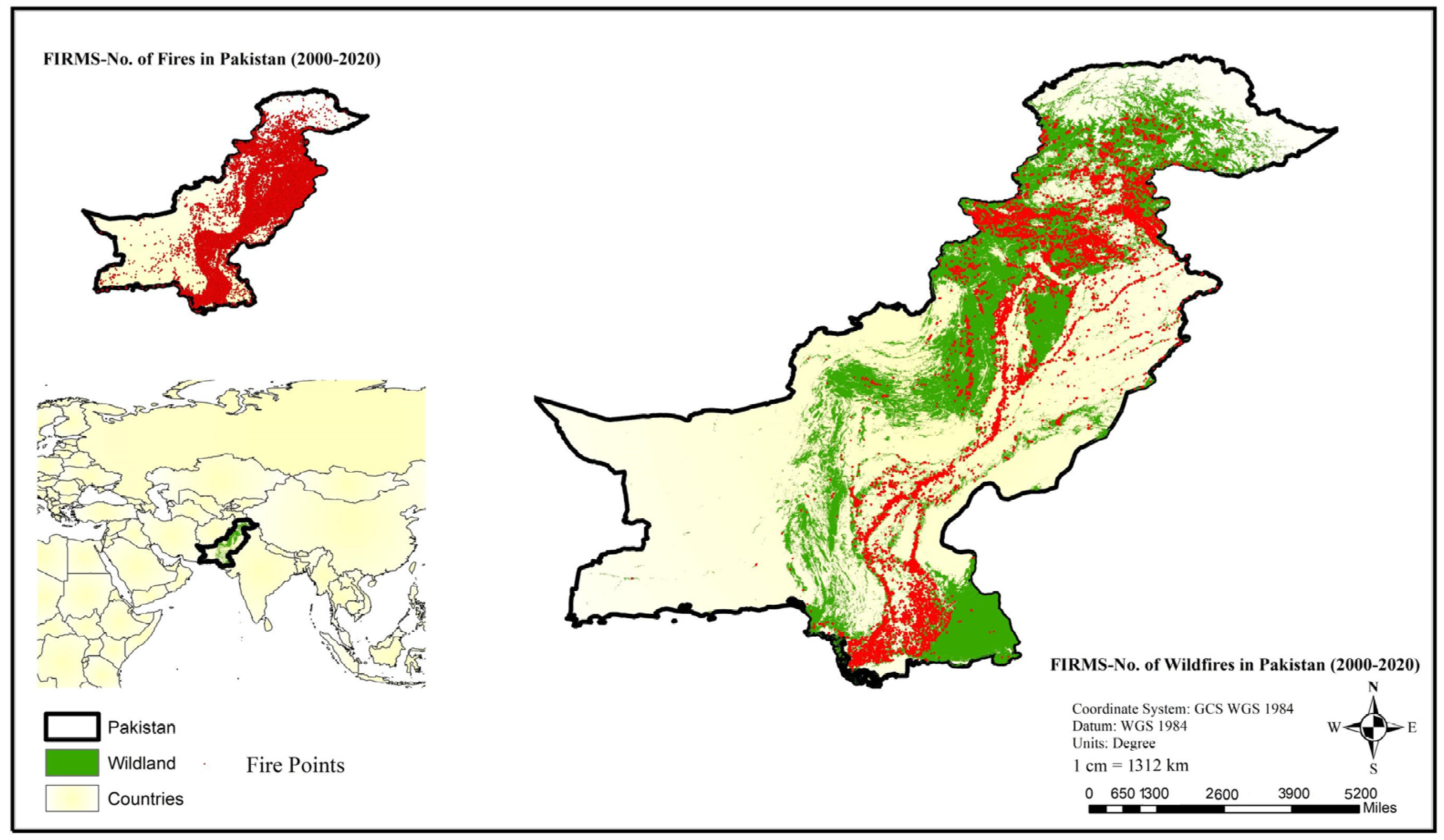
2, with a wildland area of 36.4%. Pakistan observed 175,000 fire events in this period, among which 22,311 were categorized as wildfire. Pakistan’s wildland area is shown in
Figure 1 according to land-cover classification, showing the area of interest with the overlap of historical fire events from 2001–2020. Pakistan’s eastern region is one of the most vulnerable due to its arid climate that receives the lowest rainfall and is prone to desertification. The lowest point is 0 m above sea level and the highest point is 28,251 m above sea level [
62]. The north of the country has a mountainous terrain, while the topography progressively declines southward. The northeast of the country has the largest population density. Population clusters may also be found in the vicinity of the country’s major cities, and they are scattered rather evenly across the country. The most sparsely inhabited parts of Pakistan are in the southwest. There are four seasons in Pakistan: a mild, dry winter from December to February; a hot, dry spring from March to May; a summer rainy season or southwest monsoon period, from June to August; a receding monsoon period from September to November [
63].
Due to the lack of a continuous dataset covering the whole nation, past wildfire studies were not conducted on a country level. Thanks to the development remarkable remotely sensed datasets, fire-driving variables and the best model for prediction can be examined utilizing a public worldwide dataset acquired from remotely sensed data.
Exploratory Data Analysis: Historical Fire Events
This section includes an exploratory study of Pakistan wildfires based on historical fires in the region from a definition of the major features. Other publicly available remotely sensed datasets, as well as a few more datasets created by different sectors employing satellite images, were utilized as primary features (target features/dependent variables) and driving parameters (independent variables).
The total number of fires was calculated using data from the Fire Information for Resource Management System. FIRMS provides satellite-derived near-real-time data within 3 h of satellite observation. FIRMS is a component of NASA’s Land, Atmosphere Near Real-Time Capability (LANCE) for Earth Observatory System (EOS), and it transmits data from both the Moderate Resolution Imaging Spectroradiometer (MODIS) and the Visible Infrared Imaging Radiometer Suite (VIIRS) to Terra and Aqua EOS [
64]. On the ground, the active flames displayed in
Figure 1 and
Figure 2 are represented by pixels covering 1 km
2. As a result, this pixel may include one or more fire spots within a 500 m radius. Furthermore, a variety of parameters, such as scan angle, land surface temperature, and smoke volume, impact the smallest detectable fire size. Above 1000 m
2, MODIS can identify both burning and smoldering flames; however, smaller blazing fires can be detected under extremely clear observing circumstances (50 m
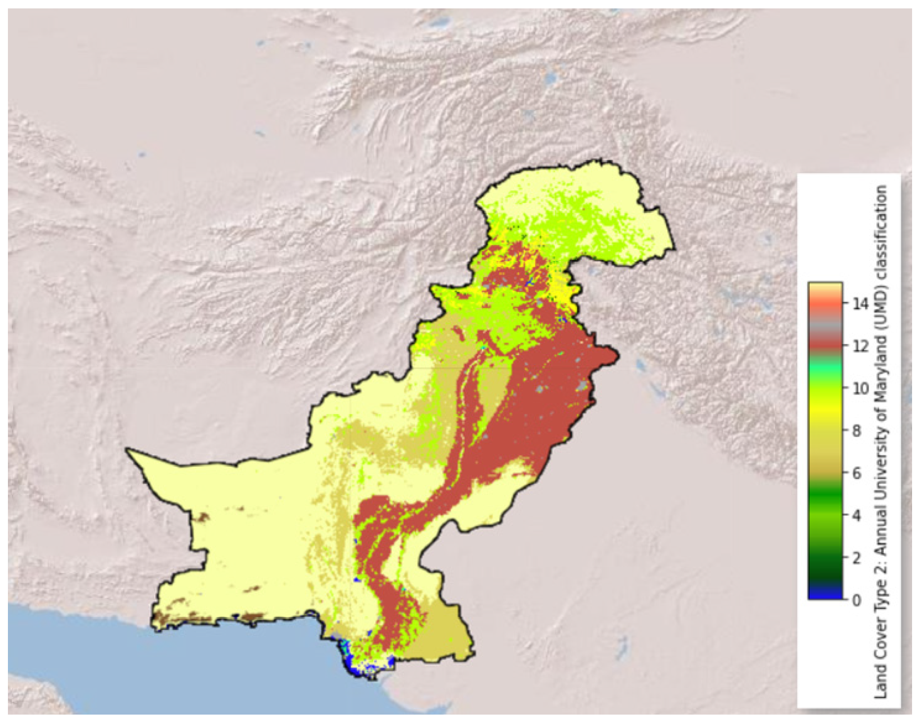
2). Active flames, such as those caused by human activity, industries, and volcanoes, can also be spotted as thermal anomalies. The FIRMS dataset includes active fire sites using the pixel value, which determines the temperature of the surface in Kelvin. At annual intervals, the MCD12Q1-V6 package gives worldwide land-cover categories (2001–2016) in Aqua and Terra. The MODIS Land Cover Type 2 Classification designed by the University of Maryland was used in this study (MODIS land cover).
Figure 2 presents the land-cover classification map for Pakistan using projection WGS84, with a global spatial coverage of 500 m. Fires that occurred in a University of Maryland Dataset (UMD)-designated region were filtered and labeled as wildfires. UMD’s landcover classification was employed as a guide, with classifications indicating shrublands, savannas, and wildlands (classes: 1–10) [
65].
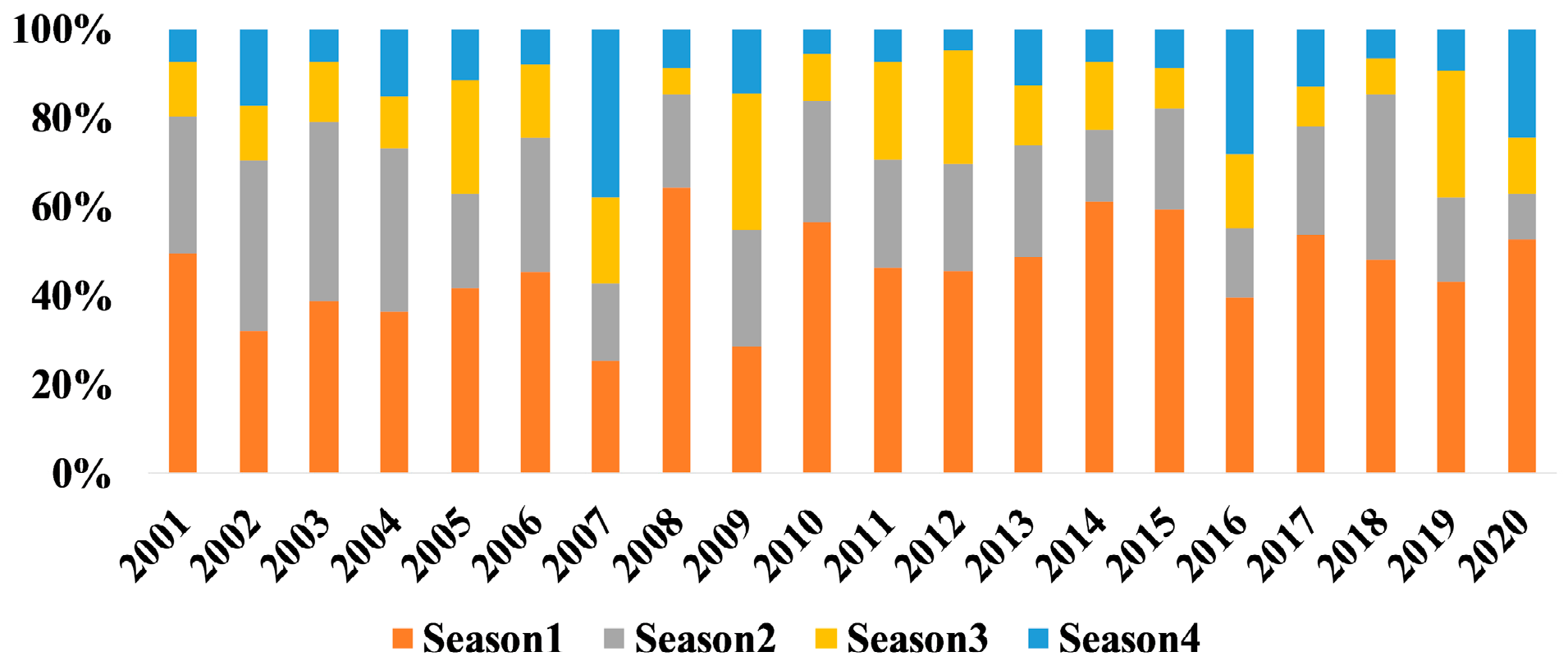
Figure 3 presents the total number of pixels representing active wildfires in Pakistan each year from 2000 to 2020. The last year, 2020, compared to the previous 20 years did not present outstanding numbers. The worst years in terms of fire activity were 2008, 2016, and 2017. More active fires were recorded in 2016, 2017, and 2018 than 2015 and 2019. A detailed overview showing the fire activity over a year is required to uncover anomalies over months. Thus,
Figure 3 shows the active wildfires over a year from 2000 to 2020 in Pakistan. The year 2008 had a significant number of active fires compared to other years. However, the satellite-driven fire data revealed that most active fires during December and January throughout the last two decades happened in all years except 2009. MODIS recorded about 10,357 active wildfire indicators over Pakistan between December and February for the last two decades.
Figure 4 shows a seasonal distribution graph of active fire locations from November 2000 to December 2020. The fire locations mostly occurred in December to February, considered as the winter season.
The basic dataset was taken from FIRMS and refined using the wildland class according to MODIS to yield the wildfire dataset (targeted features). This dataset is open to the public and provides a derived collection of data for each fire in a 1 km pixel, including fire confidence, fire kind, and temperature records. FIRMS data are available from November 2000 to the present day, with a temporal resolution of 1 day and a geographical precision of 1 km.
4. Methodology
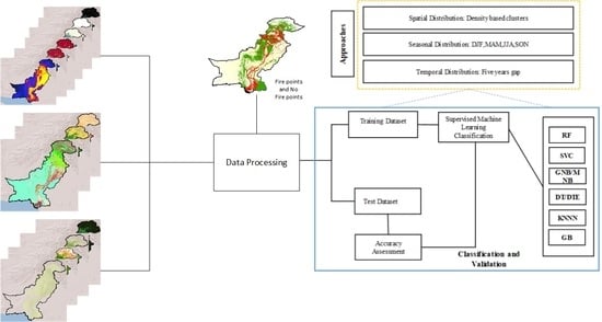
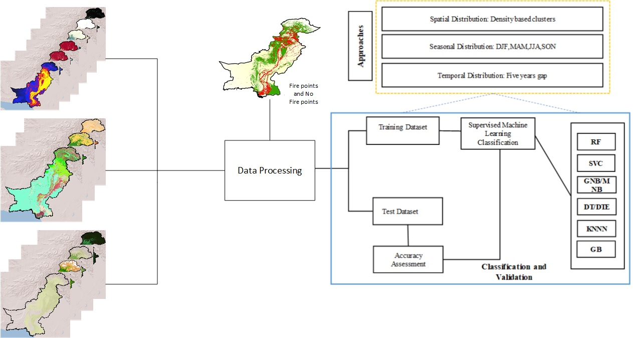
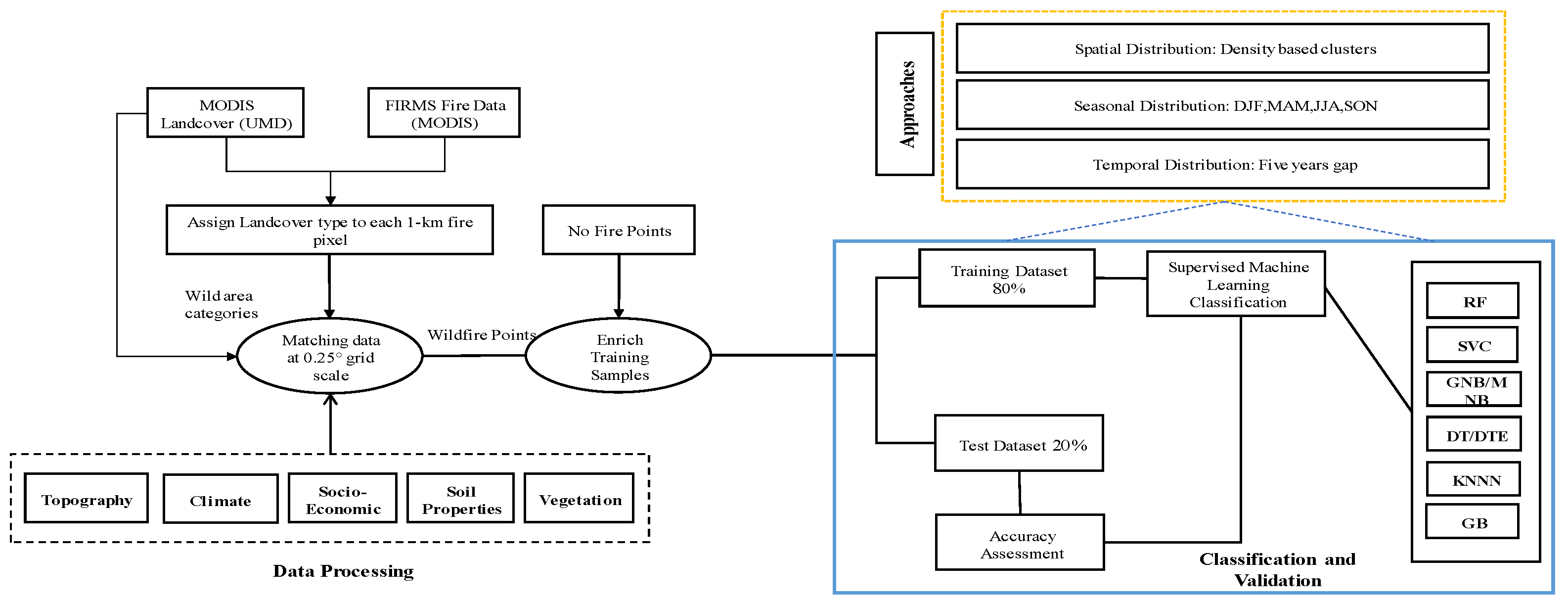
The approach utilized to achieve the study’s two primary objectives is described in this section. The first step was to establish the best fit model for fire susceptibility, and the second was to identify the driving elements that influence fire susceptibility under various situations. The methodology is broken down into three sections: (a) data preparation and preprocessing, (b) classification, and (c) validation and evaluation matrix. This structure is presented in the flowchart in
Figure 5, summarizing the essential processes employed in this study. The entire procedure was applied to the dataset in four dimensions: (1) total dataset, (2) data divided by seasons, (3) geographical data clustered on the basis of density, and (4) data divided into 5 year gaps.
The first stage was to create the training dataset, including historical fire incidents (as dependent variables or target variables) and the three primary driving elements, topography, climate, and fuel based on vegetation, soil, and socioeconomic data (as independent variables). Following that, the historical fire events dataset was split into two parts: training and testing. The training dataset was used to train ML models, and the learned model was subsequently verified using the testing dataset. For the spatial prediction of wildfire susceptibility, the best-performing ML model was employed. The chosen ML model allowed for a quantifiable evaluation of each variable’s contribution to the classification output, which was important for determining the relevance of each variable.
4.1. Data Preparation and Preprocessing
The training dataset consists of independent variables and dependent variables known as predictors and response variables, respectively. The total dataset was at the country level, with a 20 year duration, resulting in an enormous quantity of data. As a result, it was critical to automate the training dataset generation procedure. This also had the benefit of providing extra training data samples to the selected models, which improved their performance.
Targeted factors: The binary variable of fire and no-fire incidence sites served as the study’s dependent variable. As a result, mapping fire susceptibility may be thought of as a binary classification task with two classes, fire and no fire, from a machine learning perspective. As a result, an automated procedure for gathering fire and no-fire occurrence sites was devised in this study.
No-fire incidents were also collected for exploratory investigation of driving elements. In Pakistan’s wildland land-cover collection, a historical record of no fire occurrences was also created. In wildland regions, random sites with a distance of 1 km were chosen. The points that fell outside of the 1 km buffer fire zones were filtered and designated as no-fire points. Dates were assigned to no-fire points in the same range as fire data from November 2000 to December 2020, with six points assigned to each date. A total of 162 latitude and longitude points were allotted to each month. Both fire and no-fire data had the same spatial resolution. Accordingly, 22,311 fire points and 29,295 no-fire points were created for Pakistan. Each fire and no-fire record in the end file contained the “fire” property name and stored an integer-type value, where 1 signifies a fire and 0 represents a no-fire event.
Driving factors: In predictive modeling, selecting independent variables, also known as predictors or conditioning factors, is a crucial step. A total of 34 driving factors were chosen for this investigation on the basis of field observations from several studies [
66,
67,
68] and public and worldwide satellite data. Although there are no strict guidelines on which variables should be included in a model, most studies considered geomorphological, climatic, and human-related variables to be conditional factors [
69].
Wildfires are driven by three key variables, according to experts: topography, climate, and fuel. Fuel -related wildfire conditioning variables may be classified into two categories: vegetation type and socioeconomic considerations. In our research, we discovered soil-related data that may be used as fuel variables. Each of the datasets utilized in this investigation is summarized in the
Table 1. The independent variables were based on data from a remotely sensed public data archive, with some records categorized by various organizations. Remotely sensed data were used to prepare several socioeconomic variables. These data were imported as raster data, and the source column in
Table 1 gives links to data sources and data catalogs.
It has been observed by many studies that climatic datasets play a vital role in describing the factors driving wildfire. The Fire Warning Index (FWI) is a collection of NASA climate data, including temperature, humidity, and transpiration [
70,
71]. It has been used in many other areas outside Canada [
72,
73,
74,
75,
76]. Instead of limiting data models to a few parameters, we used the Terra Climate dataset [
77] and GLDAS [
78] Assimilation System (GLDAS) data with higher spatial resolution for our research, as outlined in
Table 1.
Table 1.
List and description of the study’s variable datasets with source information.
Table 1.
List and description of the study’s variable datasets with source information.
| Category | Parameter | Source | Resolution | Unit | Time |
|---|
| Topography | Elevation | NASA SRTM Digital Elevation [79] | 30 m | m | 2000 |
| Slope | ° |
| Aspect |
| Hill shadow |
| Socioeconomic | Population | GPWv411: Population Count (Population Count) | 927.67 m | Count | 2000, 2005, 2010, 2015, and 2020 |
| Human modification | CSP gHM: Global Human Modification [80] | 1000 m | km2 | 2016 |
| Travel speed | Oxford/MAP/friction_surface_2019 [81] | 927.67 m | min/m | 2019 |
| Travel speed walk |
| Settlement | GHSL: Global Human Settlement Layers [82] | 1000 m | classes | 1975–1990–2000–2014 (P2016) |
| Urban cover | Copernicus Global Land Service (CGLS) [83] | % | 2015–2019 |
| Climate | Precipitation | Global Land Data Assimilation System [78] | 27,830 m | kg/m2/s | 2000–2021 |
| Transpiration | W/m2 |
| Wind speed | m/s |
| Soil temperature | k |
| Humidity | kg/kg |
| Heat flux | W/m2 |
| Albedo | % |
| Average surface skin temperature | k |
| Soil moisture | kg/m2 |
| Actual evapotranspiration | Terra Climate: Monthly Climate global [77] | 4638.3 m | mm | 1958–2020 |
| Water deficit |
| Precipitation accumulation |
| Downward surface shortwave radiation | W/m2 |
| Minimum temperature | °C |
| Maximum temperature |
| Vapor pressure | kPa |
| Vegetation | Tree cover | Copernicus Global Land Service (CGLS) [82] | 1000 m | % | 2015–2019 |
| NDVI | MOD13A1.006 Terra Vegetation Indices (Terra Vegetation Indices) | 500 m | nm | 2000–2022 |
| FPAR | MCD15A3H.006 MODIS Leaf Area Index/FPAR0m (Copernicus.) |
| LAI | m2 |
| Land cover | MCD12Q1.006 MODIS Land Cover Type (Modis Landcover) | classes | 2001–2020 |
| Soil | Soil bulk density | OpenLandMap USDA [84] | 250 m | kg/m3 | 1950–2018 |
| Soil taxonomy | OpenLandMap USDA [85] | classes | 1950–2019 |
| Soil texture | OpenLandMap USDA [86] |
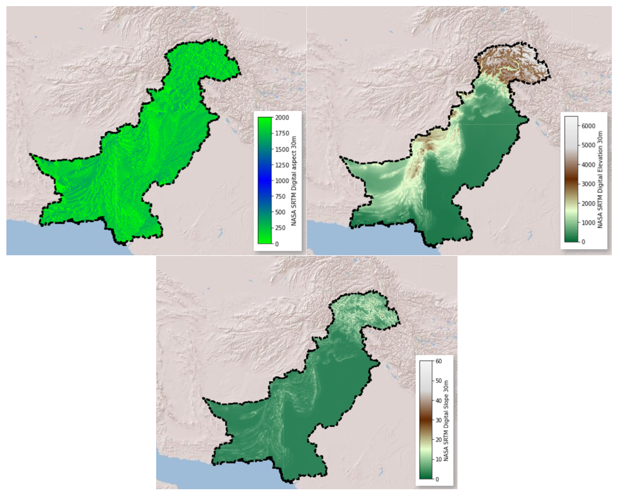
In our research, we employed a variety of derived and main climatic variables. FWI has never being used in Pakistan, and the parameters utilized in global FWI are limited. For FWI’s proposed datasets, GLDAS and Terra Climate data were picked due to their higher spatial resolution. Temperature was chosen because it has an impact on soil moisture and is linked to vegetation combustion. Elevation, slope, and aspect in
Figure 6 constituted the topographic category. The elevation was calculated using a digital elevation model (DEM) with a spatial resolution of 30 m. The model was created using a dataset obtained from NASA’s Shuttle Radar Topography Mission (SRTM) [
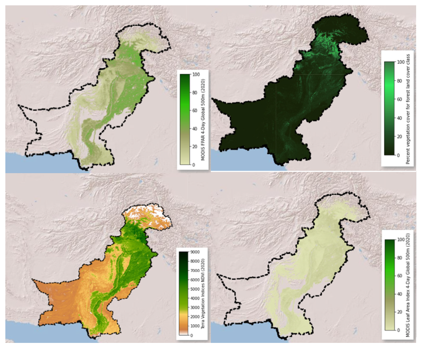
79]. DEM was used to calculate the slope or gradient of the terrain represented as an angle and aspect, commonly known as the direction in which the slope faces. Land cover, fraction of photosynthetically active radiation (FPAR), leaf area index (LAI), normalized difference vegetation index (NDVI), and tree cover were all included in the vegetation category of fuel, as shown in
Figure 7. The vegetation layer (NDVI) is directly provided by the MOD13Q1 raster product with a 250 m spatial resolution. The combined FPAR absorbed by plant canopy green components and LAI are offered by MCD15A3H-V6 level 4. The Copernicus Global Land Service (CGLS) is a multipurpose service component of the land service that delivers a number of bio-geophysical products describing the state and evolution of land surface at a global scale [
83]. The product contains continuous field layers for all basic land-cover classes, which provide proportionate estimates of vegetation/ground cover for the various land-cover categories. The tree cover fraction was calculated as a percentage of vegetation cover for the wildland from the land-cover class.
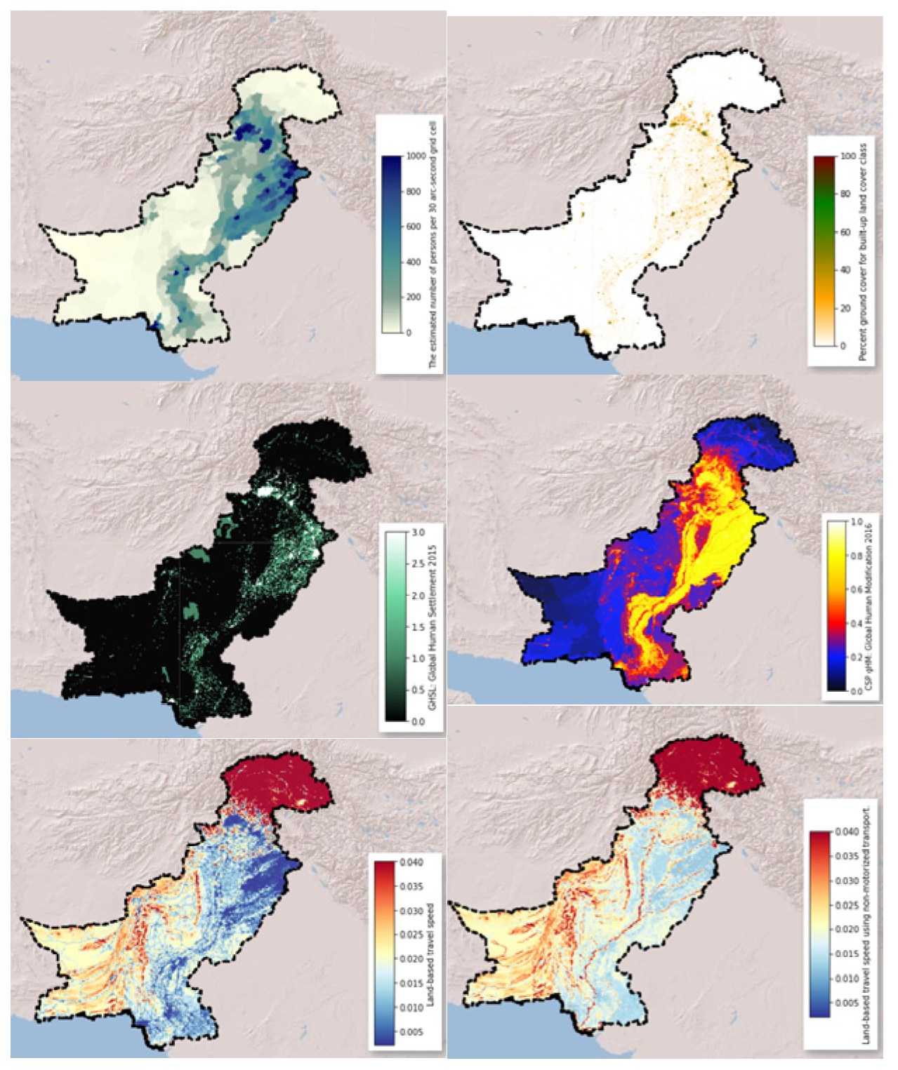
Global Human Modification (GHM) [
80], population, global human settlements, and global friction statistics were all included in the socioeconomic category, as presented in
Figure 8. The GHM dataset provides a global assessment of human alteration of terrestrial areas with a spatial resolution of 1 km. The GHM values range from 0 to 1 and are linked to a certain type of human alteration, sometimes referred to as a stressor. Human habitation, transportation, mining, and energy generation are examples of important anthropogenic stresses. The World Pop dataset estimates the number of people living in 85 million grid cells (population count). The degree of urbanization for 2015 was provided by the Global Human Settlement Layer. The degree of urbanization divides a country’s total area into urban and rural zones for the year 2019. The global friction surface enumerates land-based travel speed for all land pixels between 85° north and 60° south. It also includes “walking only” travel speeds, which are achieved by relying solely on nonmotorized modes of transportation [
81]. A proportionate distribution of population from census and administrative units was used to disperse people to cells.
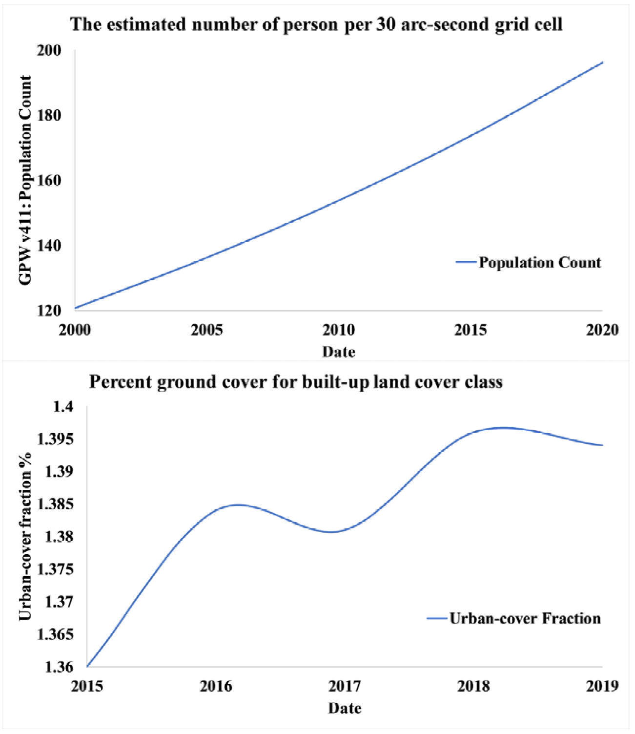
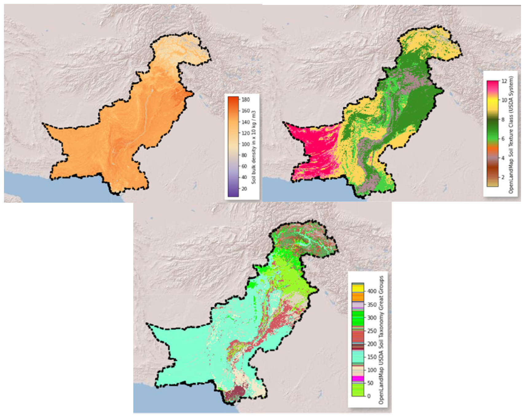
According to national censuses and population records, these population count grids included estimates of the number of people every 30 arc-second grid cell. Each 5 year gap was represented by a single picture. Percentage ground cover for the built-up land-cover class was chosen as the urban cover fraction from the CGLS. There was a continuous growth in per pixel population of Pakistan by year; hence, the built-up area increased.
Figure 9 gives a picture of growing population per pixel from year 2001 to 2019, as well as the annual change of built up area from 2015–2019. Soil data included soil texture classes (USDA system), soil great group, and soil bulk density (fine earth) 10 × kg/m
3 at 0 cm depth with 250 resolution, as presented in
Figure 10 [
84,
85,
86].
The training dataset, which was enriched by predictor variables, was constructed after the fire and no-fire training points were formed and conditional factors were preprocessed. The 34 independent variables were first acquired and resampled with the same spatial resolution. After that, information extraction was used to populate the table with predictor values and create training samples for each latitude and longitude. As a result, a dataset of fire and no-fire sites was produced, with driving variable information stored against each latitude and longitude.
4.2. Classification
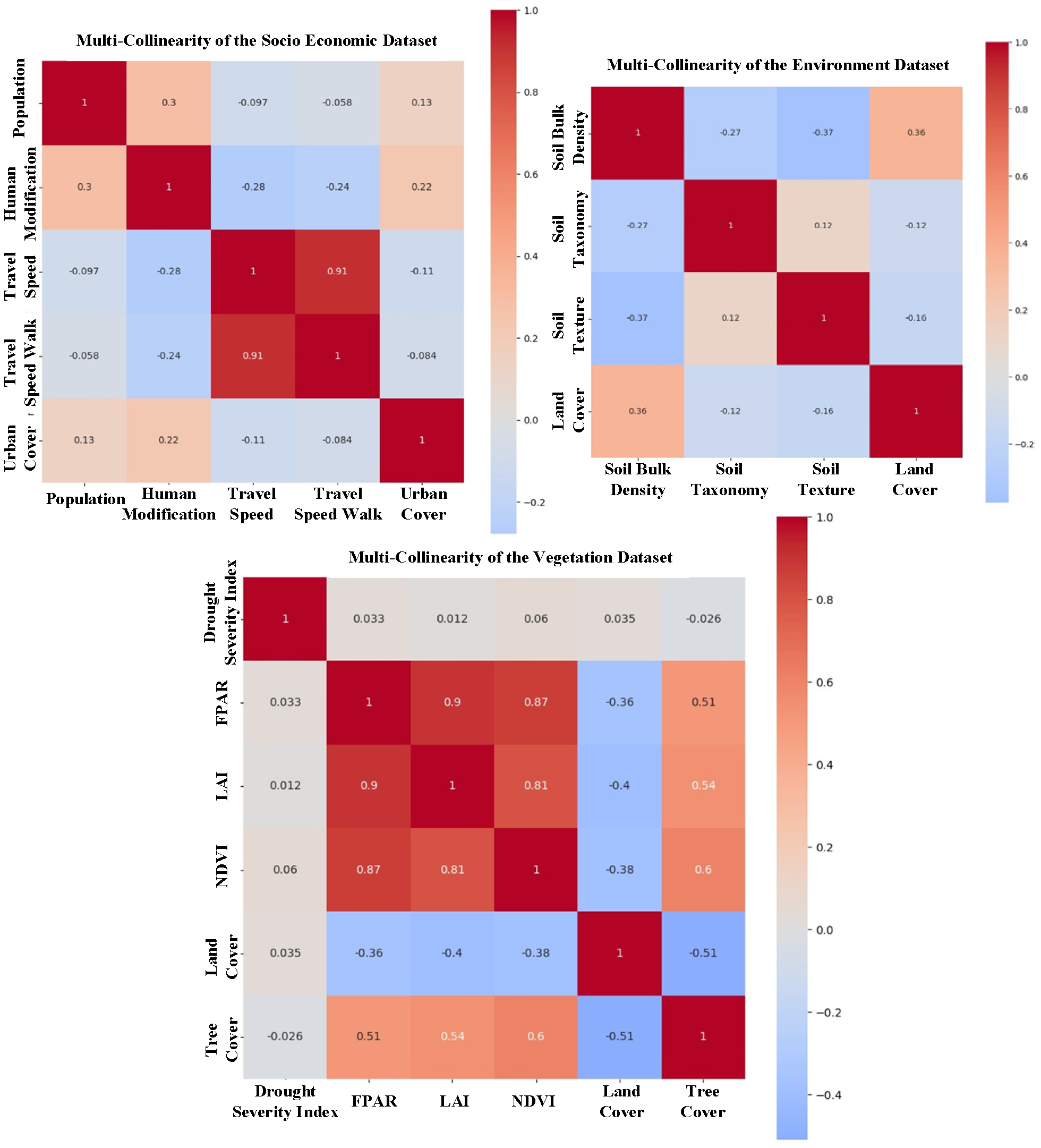
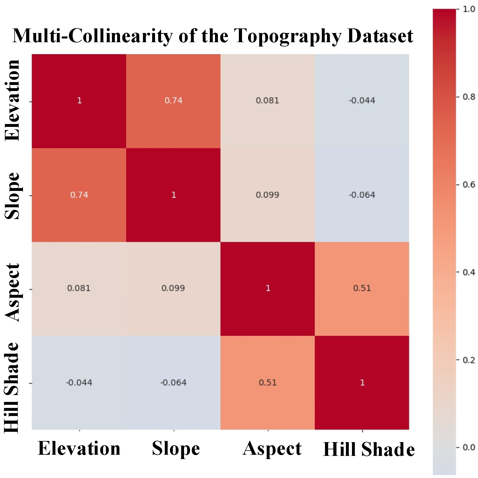
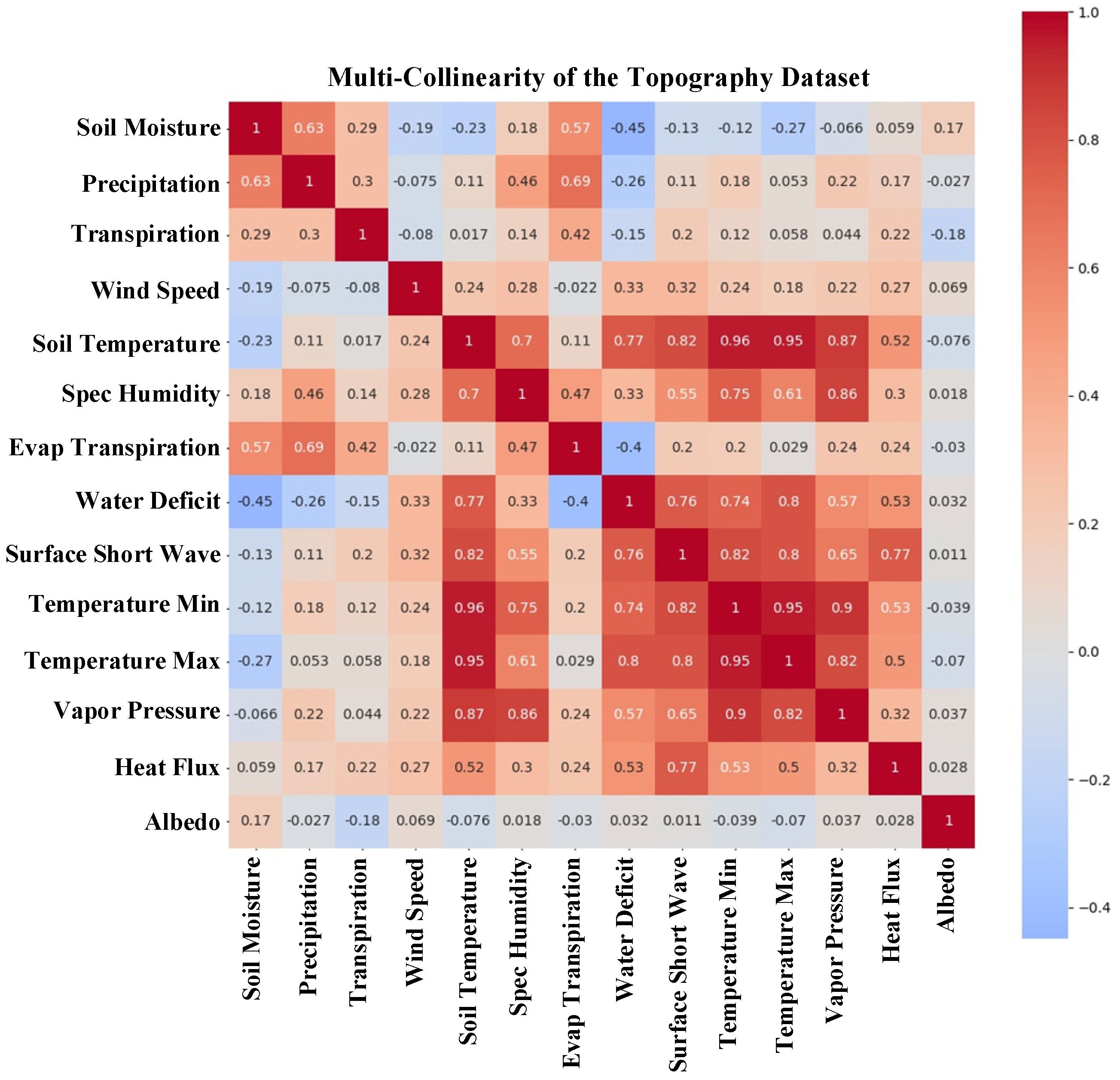
The next stage was to assess the classification accuracy after the training set was prepared. Input training samples are widely used in supervised classifications. Prior to fire modeling, it is critical to conduct a multicollinearity study. To identify any linked components, a multicollinearity analysis was used. If some elements are not adequately chosen, correlation may occur, and those components should be modified or deleted. The next step was to conduct a multicollinearity analysis to determine the association between the predictor wildland fire variables. In the prediction of fire susceptibility, feature selection is very crucial.
The Spearman rank correlation test is a nonparametric test used to determine the degree and direction of the connection between wildfire explanatory variables (positive or negative). The entire negative and positive linear correlation is represented by Spearman’s rank correlation coefficient, which ranges from −1 to 1. Spearman’s correlation coefficients for the three categories of wildfire explanatory variables were computed individually.
Figure 11,
Figure 12 and
Figure 13 show the correlation among all groups of data. Each cell in the correlation matrix indicates a “correlation coefficient” between the two variables corresponding to the row and column of the cell. In the correlation matrix of the topography dataset, a large positive correlation (0.74) was indicated between elevation and slope, i.e., if the value of one of the variables increased, the value of the other variable increased as well. In the correlation matrix of socioeconomic data, a large positive correlation (0.81) was indicated between travel speed and travel speed by walking. In the correlation matrix of vegetation data, a large positive correlation was indicated between NDVI and FPAR (0.87), between NDVI and LAI (0.81), and between FPAR and LAI (0.9). In the climatic dataset, the temperature minimum and temperature maximum showed a correlation of (0.91) with soil temperature. Furthermore, the temperature minimum and temperature maximum were also correlated (0.95). Most values were near to 0 (both positive and negative), indicating the absence of any correlation between those variables and, hence, their independence.
To create wildland fire susceptibility maps, RF, SVM, DT, KNN, GB, and NB classifiers were used. RF [
87] is an ensemble learning approach based on the construction of many classification trees, the results of which are aggregated to estimate a classification. RF uses bootstrapping techniques to exploit random binary trees using a subset of observations. A random sample of training data is taken from the original dataset and utilized to develop the model [
87]. The benefit of employing RF is that the data utilized seems random and diversified, which produces more accurate findings than individuals.
SVM is a nonparametric kernel-based model that is one of the most widely used classification algorithms [
88]. It is the most effective at addressing complicated, resilient linear and nonlinear classification and regression problems [
89].
NB is a machine learning model based on the Bayes theorem seldom employed in air pollution prediction when compared to the techniques discussed [
90]. The usage of NB, on the other hand, is more adaptive for multiclass prediction. NB presupposes that the presence of one characteristic in a class is unrelated to the presence of another. As a result, each trait has an equal and independent impact on the chance of a sample belonging to a certain class. NB is quick, simple to design, and good for large datasets.
The KNN technique is a nonparametric model for classification and regression applications that uses lazy learning [
91] to avoid making assumptions about the data. As a result, without universal predictors, this model is critical for air pollution prediction. The KNN technique starts by establishing at random k number of class centers, categorizing the training data on the basis of their closeness to these class centers, repeatedly relocating the class centers to the middle of the training data, and reclassifying the data
GB techniques [
92] have become more popular in recent years, thanks in part to the creation and distribution of open-source tools. The loss function used to train these models is a fundamental component of gradient boosting, and the options for these functions are mainly limited to those that prioritize strong prediction of the distributional bulk rather than the tails.
DT belongs to the class of supervised learning algorithms and is another example of a universal function approximator, although such universality is difficult to achieve in its basic form [
87]. DT can be used for both classification and regression problems. A DT is a set of if–then–else rules with multiple branches joined by decision nodes and terminated by leaf nodes. The decision node is where the tree splits into different branches, with each branch corresponding to the particular decision being taken by the algorithm, while leaf nodes represent the model output.
Classifiers other than RF such as SVM, NB, and KNN still have the flaw of not examining the relevance of the variables, i.e., variable importance. Furthermore, the probability function is solely provided by the RF classifier. Equation (1) represents the normalized feature importance.
where
is the normalized importance of feature
, and
is the importance of feature
,
all features.
4.3. Validation and Evaluation Matrix
The trained ML models could forecast the location of a fire; nonetheless, it was critical to assess their performance. As a result, an accuracy evaluation was carried out. For model validation, the sample dataset of fire and no-fire locations was separated into training and test datasets. The points were distributed in an 80:20 ratio for training and testing. The testing dataset was subjected to the accuracy evaluation, which was based on a confusion matrix. The total accuracy was calculated using predicted and actual points difference.
Accuracy Assessment of ML Algorithms: The performance of the ML models was assessed using a commonly accepted accuracy evaluation approach. The accuracy assessment characteristics, such as overall accuracy, AUC score, and precision score, provide a general understanding of how the model performs. Using the independent testing datasets acquired from the sample dataset, the accuracy evaluation was generated. This sample dataset was divided in an 80:20 ratio, which meant that 80% of the data were used to train the model, while 20% of the data were used to test it. Accuracy refers to how effectively a binary classification test properly detects or eliminates a condition. That is, the proportion of correct predictions (including true positives and true negatives) among the total number of instances evaluated is the accuracy [
93].
where
is true positive,
is false positive,
is true negative, and
is false negative. The number of true positives divided by the total number of true positives and false positives indicates the precision. In other words, it is the total number of positive class values predicted divided by the total number of positive predictions.
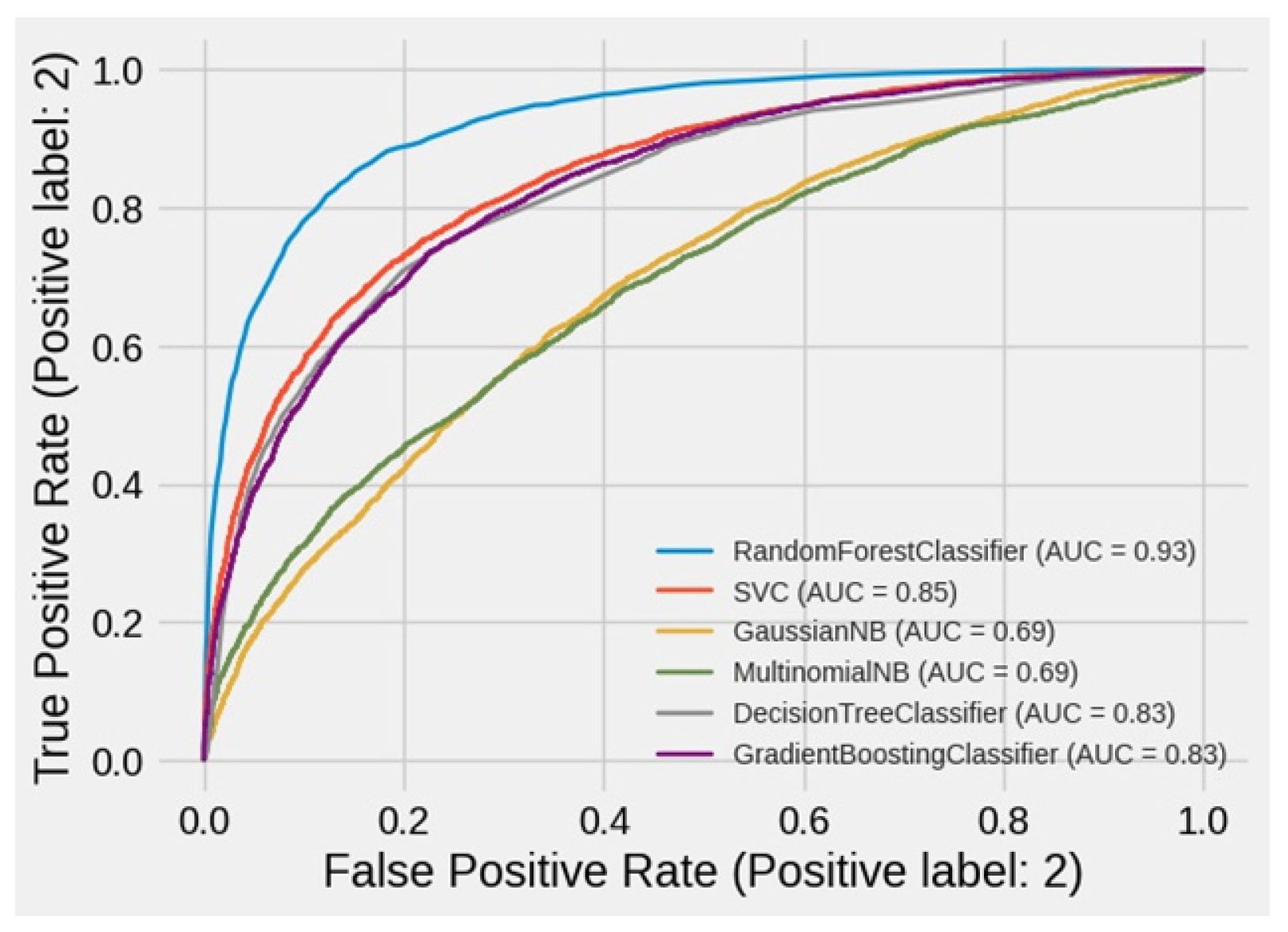
Figure 14 represents the area under the curve (also known as the AUC), which is equal to the likelihood that a classifier would rate a randomly chosen positive instance higher than a randomly chosen negative instance when using normalized units (assuming that “positive” ranks higher than “negative”) [
91,
94].
5. Results
This section highlights the study’s results depending on the technique used. The findings of the fire occurrence sites acquired from the FIRMS dataset are presented in the first part. The outcomes of the various ML algorithms are revealed in the next half of this section, where the utilized prediction variables were acquired on a large scale from public platforms.
Supervised ML algorithms, RF, DT, SVM, GB, and NB, were trained with an 80% training dataset that included 8924 test samples. There were 22,311 fire points and 22,311 no-fire points in the samples with two classes. The accuracy of the ML models is summarized in
Table 2. The RF model had the highest accuracy (85.19%), while the NB model had the lowest accuracy (57.66%). The accuracy of the SVM, DT, and KNN models was 75%, somewhat lower than the RF model, but they all outperformed the NB model. In comparison to the prediction of the fire class, the assessment found that all methods typically performed well for predicting the no-fire class.
The NB and DT models were unable to handle missing data in categorization. This can happen when working with raster-formatted predictive factors. There may be a few blank cells in these rasters, indicating a lack of data. As a result, a vector dataset was created.
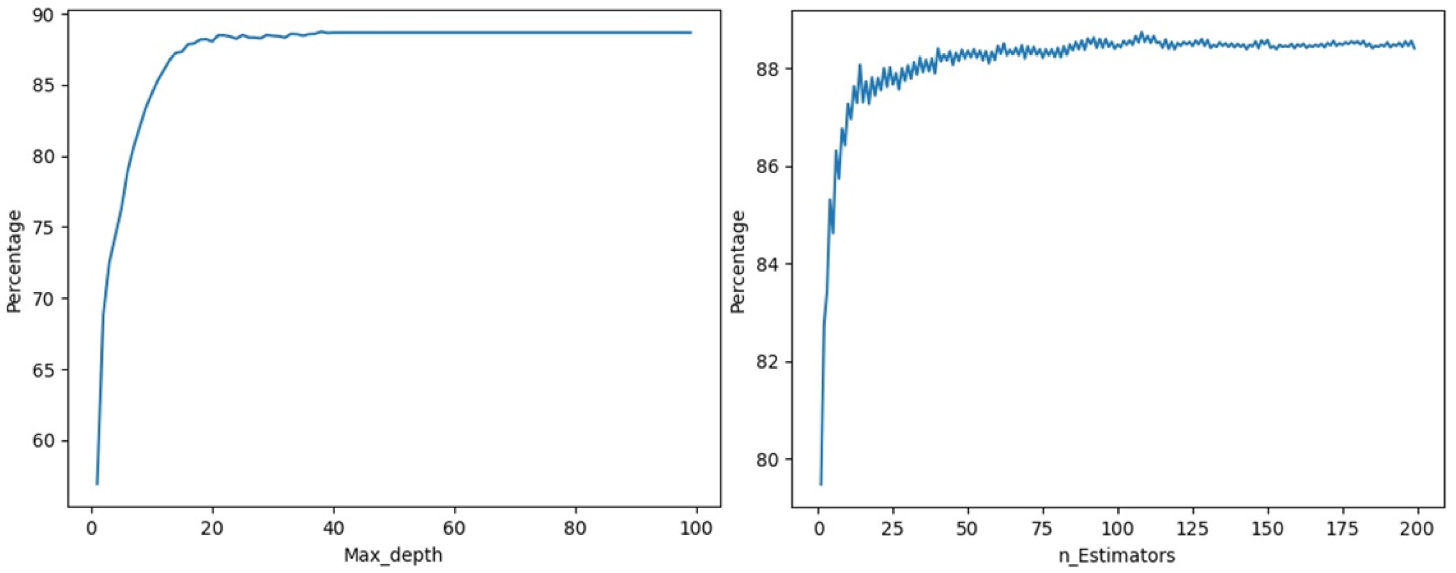
The accuracy assessment script with the RF algorithms was executed multiple times to find the proper number of the maximum trees and the depth for the RF model. This was an essential step, as these numbers have a direct impact on the accuracy of the model. Additionally, it can also reveal how many leaf nodes are important to implement when two classes are classified. Hyperparameter tuning is the process of determining the right combination of hyperparameters that allows the model to maximize model performance. Setting the correct combination of hyperparameters is the only way to extract the maximum performance out of models. In manual hyperparameter tuning, different combinations of hyperparameters are set (and experimented with) manually. This is a tedious process and cannot be practical in cases where there are many hyperparameters to evaluate.
The accuracy of the RF model increased with the number of leaf nodes until it reached 108 leaf nodes and a depth of 38, as shown in
Figure 15. The model’s accuracy was nearly consistent over more than 108 leaf nodes.
Figure 15 shows the results of the RF model, which demonstrated that, as the number of trees increased, so did the accuracy. As a result, in this investigation, the best number of trees used in the RF model was 108 trees. Thus, in this investigation, the ideal number of trees in the RF model was 108 trees with a maximum depth of 38, giving 88.74% accuracy, as presented in
Table 3.
It was necessary to verify if the RF outperformed other models in temporal, spatial, and seasonal settings. This can contribute to the model’s overall dependability. According to research, the model always produces varied findings depending on the region. Additionally, the temporal validity of models should be determined. The entire dataset was divided into categories and subcategories to make the model more usable in a real-time context.
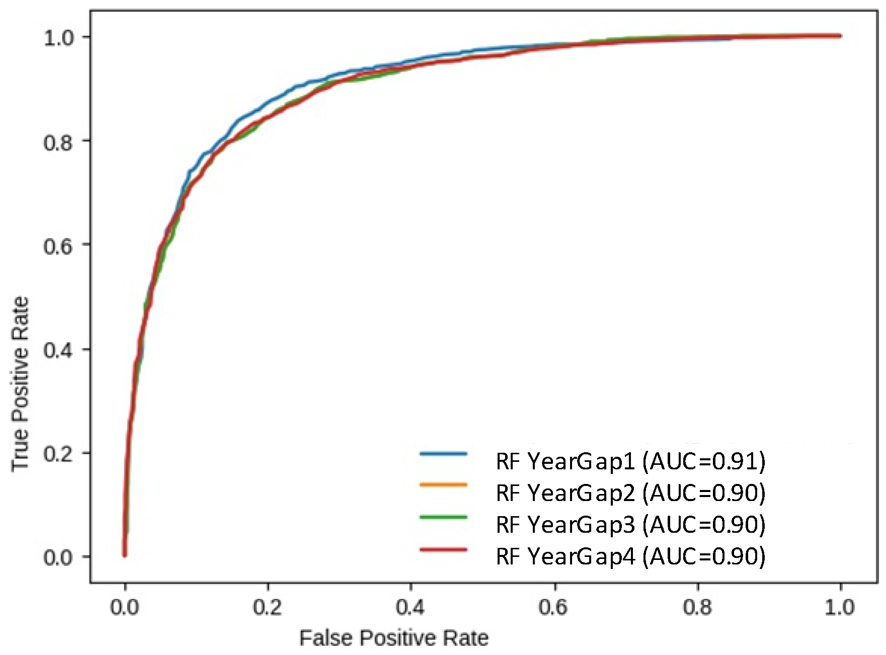
Temporal relatability of model: What time period should be employed for model training is a typical concern in data-driven problems. Due to the stochasticity or heterogeneity of data, a model trained on short-term data may produce significant uncertainty, but a model developed on long-term data may smooth out the behavior tendency when applied to current data [
95]. To see if the model remained the same over a long period of time, the entire dataset was separated into four groups, each with a 5 year hiatus. The years 2000 to 2005 were designated as Y1, along with 2006 to 2010 as Y2, 2011 to 2015 as Y3, and 2016 to 2020 as Y4. Because data for the year 2000 were only accessible from November onward, there were fewer samples available in Y1 than in other gaps.
It was observed in all year gaps (temporal variation) that RF outperformed the other models.
Figure 16 and
Table 4 show that the RF accuracy assessment remained the best for Y1 with an AUC value of 0.91 and accuracy score of 84.74%.
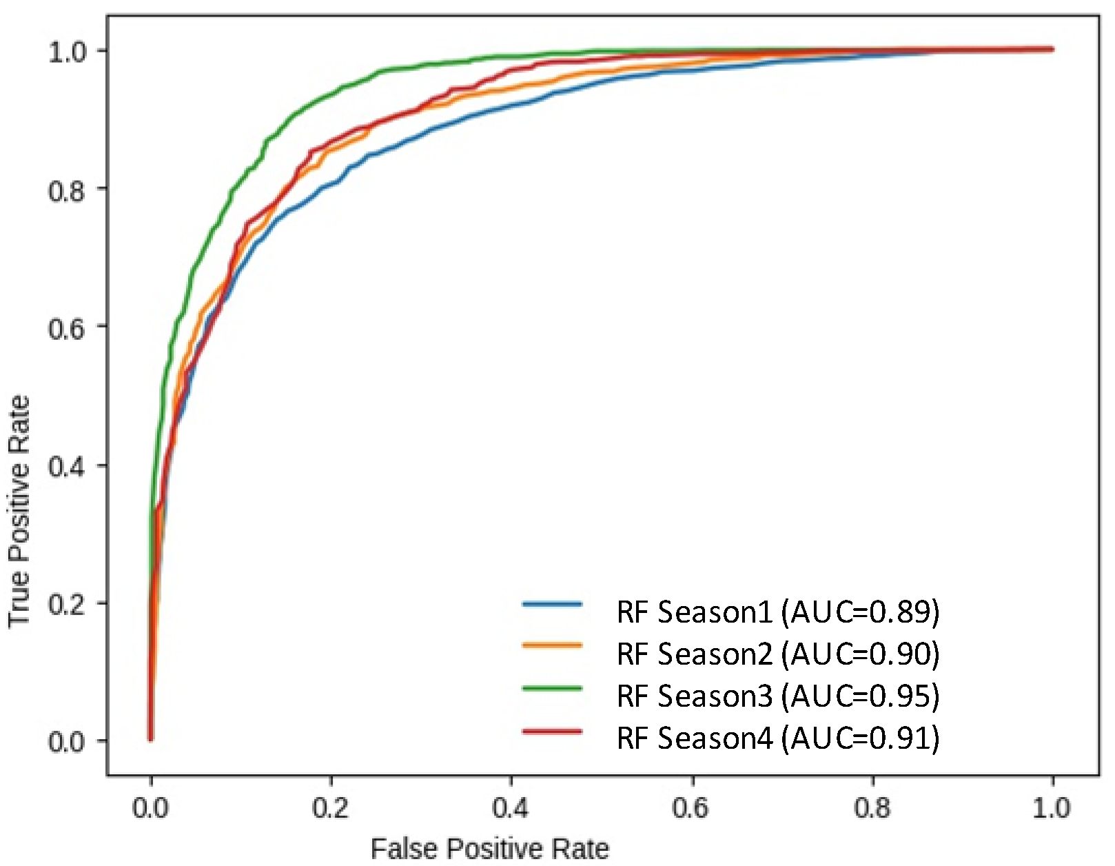
Seasonal accuracy assessment: There are four seasons in Pakistan: a mild, dry winter from December to February; a hot, dry spring from March to May; a summer rainy season or southwest monsoon period, from June to August; a receding monsoon period from September to November. As a result, the dataset was divided into four seasons.
It was observed in the seasonal division comparison that RF still outperformed other models.
Figure 17 and
Table 5 show that the RF evaluation factors remained the best for season 3 with an AUC value of 0.95 and accuracy of 89.25%.
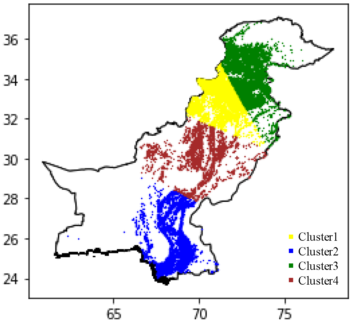
Spatial relatability of model: Although the data-driven strategy was studied at the country scale, the relative features showed considerable distinction for different clusters in Pakistan, as shown in
Figure 18. To investigate if the driven data variation resulting from spatial variation had a significant influence on the fire occurrence, four density-based clusters with distinct features were chosen for analysis. K-means is a simple technique for clustering analysis. Its aim is to find the best division of
n entities into
k groups (called clusters), so that the total distance between the group’s members and corresponding centroid, irrespective of the group, is minimized. Each entity belongs to the cluster with the nearest mean. This results in a partitioning of the data space into Voronoi cells. We used K-mean clustering for spatial location to divide the dataset into four density-based clusters [
96].
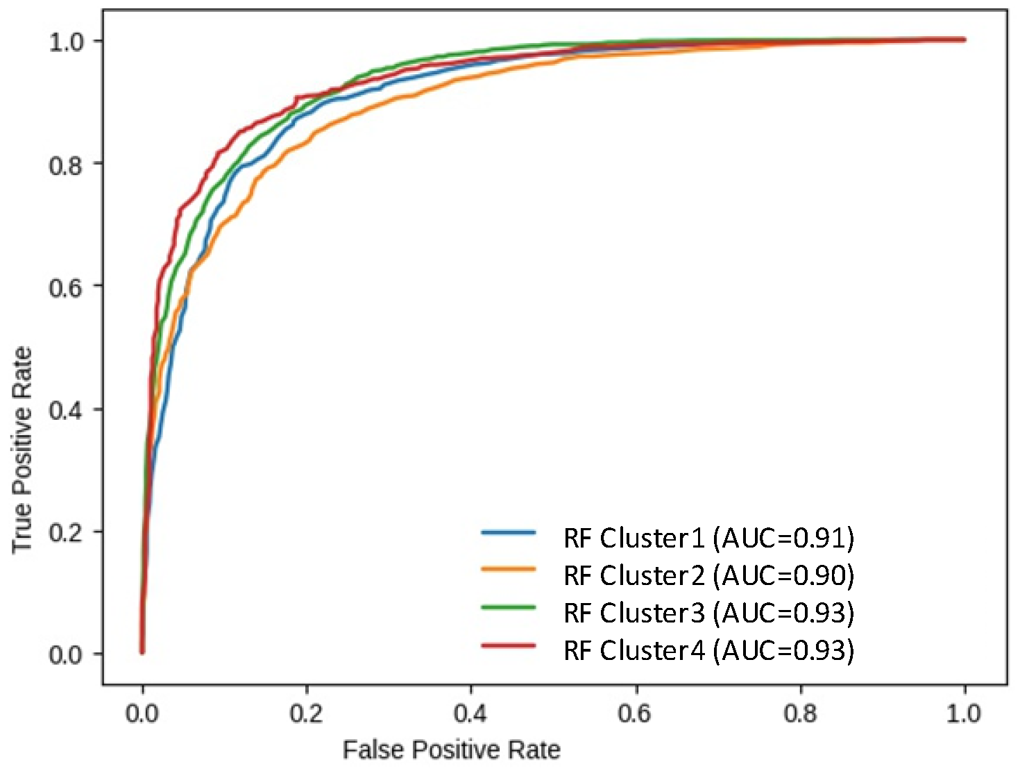
It was observed in the locational division comparison that RF still outperformed the other models.
Figure 19 and
Table 6 show that the RF accuracy assessment remained the best for cluster 4 with an AUC value of 0.93 and accuracy of 86.18%.
6. Feature Importance: Driving Factors
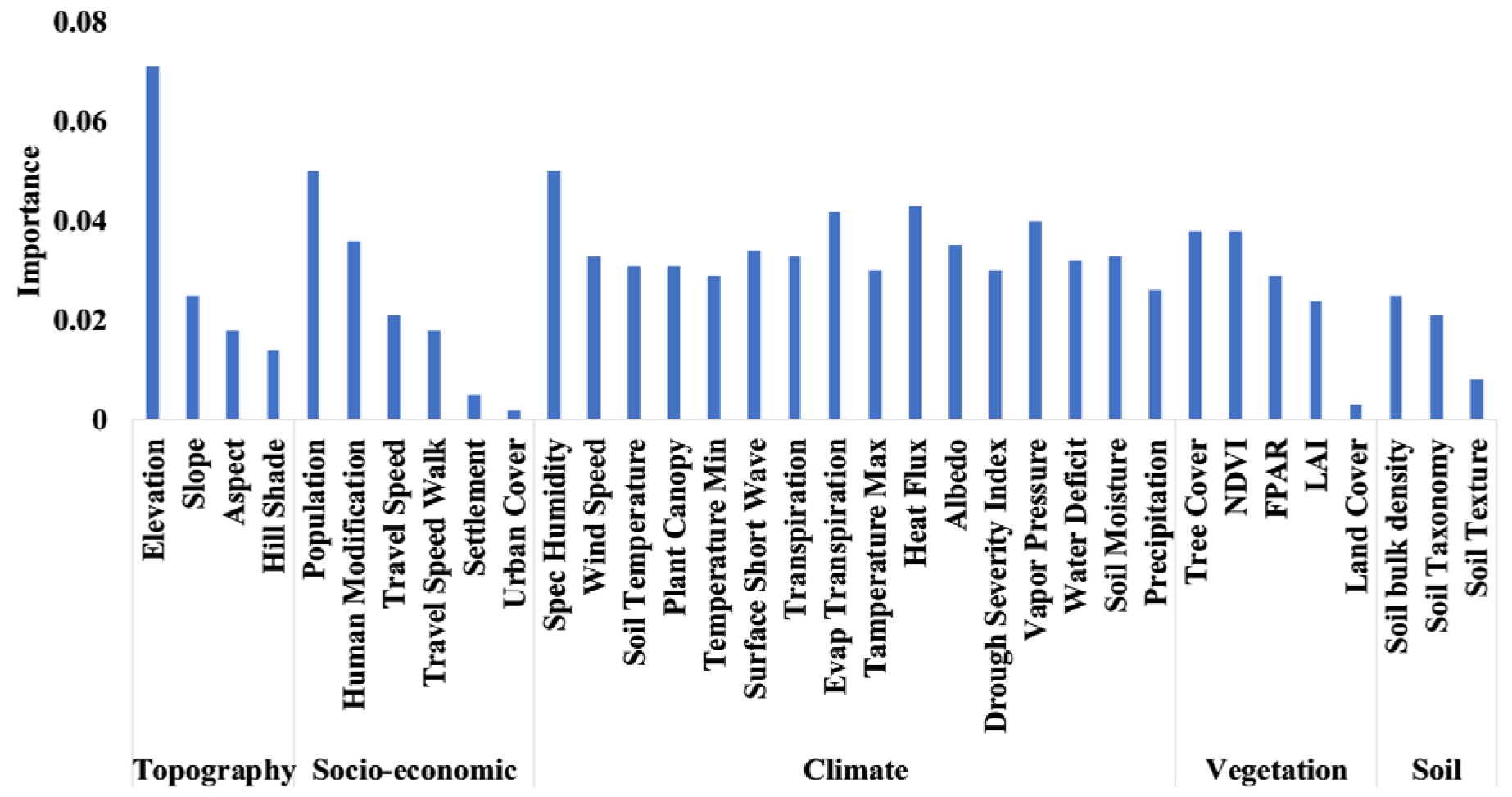
In comparison to other ML models such as NB, DT, and SVM, the RF model achieved superior accuracy. As a result, it was picked as the most relevant and appropriate ML model for this research. This approach allowed for a quantitative assessment of each variable’s contribution to the classification result, which is important for determining the variable’s relevance. The training dataset was used to determine the variable significance. Using the RF model,
Figure 20 depicts the most critical wildfire conditioning elements from 2000 to 2020. Elevation and population, as well as particular humidity, were the most essential characteristics recognized as “key drivers”. Settlement, land cover, and urban cover were the least important but still essential determinants.
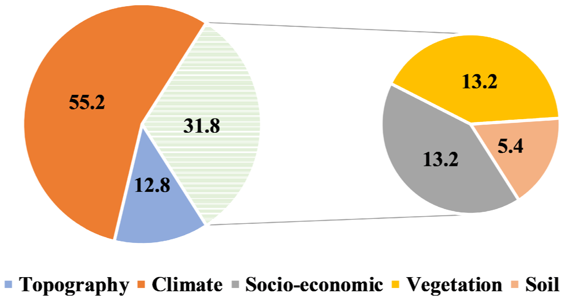
Figure 20 also presents the importance of each variable. The percentage share of climatic factors was 55.2%, while fuel and topography factors contributed to 31.8% and 12.8%, respectively, as shown in
Figure 21. The fire hazard can be predicted using static (long-term) and dynamic (short-term) indicators on the basis of this variability [
56]. Static indicators rely on elements that do not change over time, such as topography and vegetation type. These are mostly utilized for long-term planning for fire, such as decisions regarding the construction of protective infrastructure. Hence, this shows that the model can be used for long-term planning.
Because the model’s accuracy varied by season, annual gap, and locational cluster, it was obligatory to investigate the relevance of features in each of the three groups and their subgroups in order to differentiate subareas, as well as to train the model with the corresponding database.
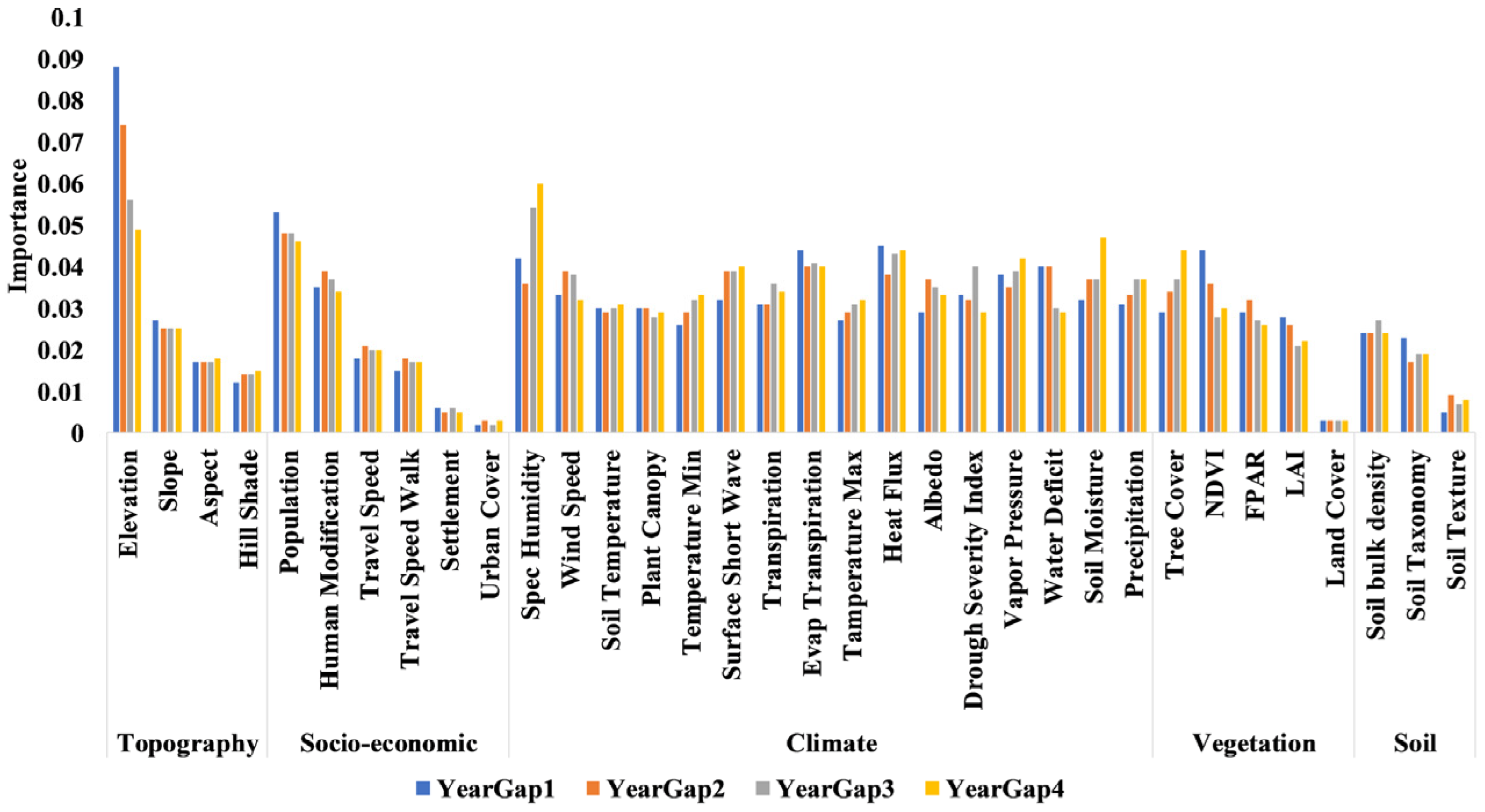
Temporal feature importance analysis: The most essential element in year gaps Y1, Y2, and Y3 was elevation, but in a more recent year gap (Y4), it was discovered that particular humidity had the most critical influence, with height coming in second. Fuel, i.e., socioeconomic considerations, were shown to be just as relevant as topographical and meteorological elements in all years, as presented in
Figure 22.
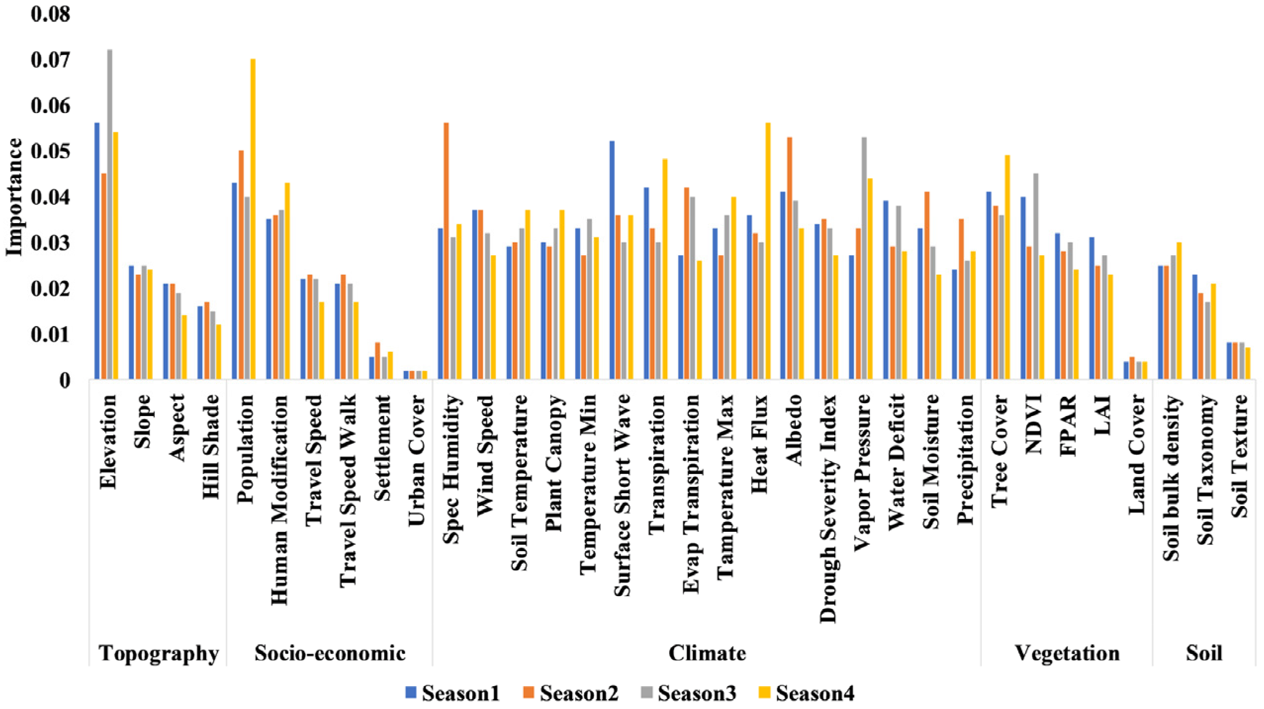
Seasonal feature importance analysis: Elevation was the most important driving factor in Seasons S1 and S2, whereas, in Seasons S3 and S4, population and specific humidity were more essential, with elevation coming in second. Seasonal differences in feature prominence were detected as presented in
Figure 23.
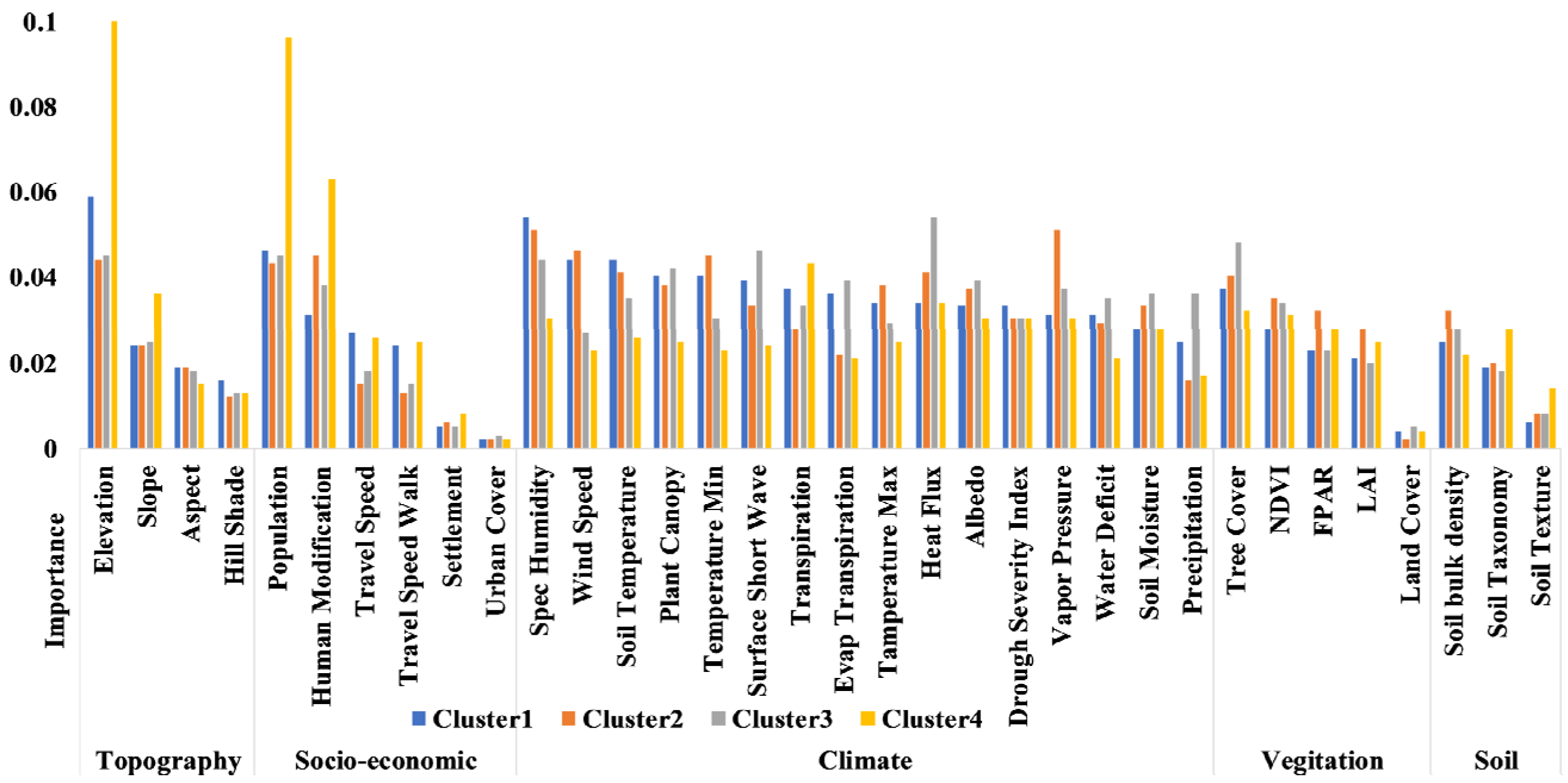
Spatial feature importance analysis: From a management standpoint, it is necessary to establish regional-level management rather than a country-level forecast, so that all states and provinces can construct their own wildfire readiness profiles to spatially analyze the area at risk. Better management can be achieved, according to our research, if policymaking is more refined on a spatial scale; rather than merely at the level of states/provinces, this can be achieved at the level of cities with a history of wildfires. Each subarea should develop its own wildfire control system, according to the recommendation.
In clusters C1 and C4, the most important feature was elevation, whereas, in clusters C2 and C3, vapor pressure and heat flux played most important role, and elevation took second place. A high variance of feature importance was observed across clusters, as shown in
Figure 24.
7. Discussion
The primary goal of this study was to get a grasp on how to generate a fire occurrence and no-fire dataset from a historical inventory so that it could be incorporated into machine learning models for wildfire prediction and analysis of driving factors. Many previous studies employed a 1 km resolution dataset from FIRMS for fire incidence points. No-fire points, on the other hand, were not discussed. Constructing no-fire points is necessary for a greater understanding of fire points. Thus, in the UMD-categorized wildland region, this study proposed a unique and automated technique for collecting samples of no-fire occurrence areas across Pakistan with the same 1 km resolution. Fire occurrence points that overlapped with no-fire occurrence sites were eliminated. As a result, a greater number of no-fire occurrence sites were employed. Many previous studies employed a 50/50 split, which increased the accuracy ratio and reduced the model’s accuracy in real-time situations. We utilized a combination of 50% fire points and 50% no-fire points for training. We relied on 1 month average values of daily datasets to retain all accessible data when producing datasets because certain values were missing against each date. As a result, 1 month was chosen as the minimum time frame for all driving elements.
The study’s second goal was to examine alternative machine learning algorithms, with the top-performing model being utilized to map the fire incidence likelihood. Six machine learning techniques were applied to the testing dataset and verified. The findings showed that the RF model produced the best outcomes, whereas the multinominal NB model produced the worst results. The RF model’s high degree of precision was likely due to the model’s composition of many separately trained decision trees, each of which generates a classification decision in which the class with the most votes is chosen as the final classification rules for the input data. As a result, as indicated by [
97,
98], this strategy is suggested for future deployment of fire management decision systems. In order to improve accuracy, the RF model’s number of trees and maximum depth were tweaked. The model with 108 trees and a maximum depth of 38 achieved the best results. However, when additional predictive factors are incorporated, the number of trees in the model may expand. As RF can handle several variables efficiently, the variable relevance of the 34 variables was analyzed to determine the contribution of each variable. Upon removing any of these factors, the accuracy rate of the classifier decreased. As land cover is a significant component, it was surprising that it did not have a greater relevance score. This can be explained by the type of land-cover data utilized in the study, which included a wide variety of data. Land cover was also utilized to filter out fires that occurred solely on wildland. As a result, wildland type modifications, such as grassland savannas or shrubs, did not have a significant effect in fire incidence. The same reasoning can be applied to other less important driving factors such as urban cover and human settlements. However, it was found that human settlements and urban cover were still present in wildland areas, playing role in fire occurrence.
The dimensionality of input variables can be adjusted using methods such as principal component analysis, which reduces the number of input variables while retaining the least amount of information and reducing data redundancy. In order to understand how the model is influenced, the model can be modified by deleting the lowest-ranked conditioning variables with no importance. This model was used to construct a susceptibility map that depicted the likelihood of a region being affected by wildfire. Despite this, wildfires are architecturally complicated and have a wide range of physical characteristics. We attempted to use as many publicly available datasets as possible. Every dataset was discovered to play a role in the incidence of fires. As a result, incorporating additional essential components can enhance the complexity of the model, resulting in a likely increase in accuracy. We treated the accuracy gap as the lack of certain other important factors in order to make the model more usable in real-time scenarios. This emphasizes the significance of data sharing and infrastructure development in order to discover more factors that contribute to wildfire incidence. Validating the stability of machine learning models is always necessary. The train/test split methodology was employed in this study as the most popular validation method. Furthermore, the testing sample was generated at random, reducing the danger of sampling bias. Due to the open availability of datasets and processing techniques in the cloud environment, this development creates tremendous prospects for research platforms. All datasets created by various organizations and made available give a fantastic opportunity for developing nations such as Pakistan to access and analyze the data for improved wildfire control and mitigation. It is challenging to manage a large number of datasets using traditional methods and tools. In contrast, machine learning is a simple and reliable categorization approach for exploration. All emerging countries can analyze the catastrophic risk using global datasets that are freely available.
8. Conclusions
Illustrating the exploratory investigation of previous fire incidents is critical. Within the research period of November 2000 to December 2020, the analysis of Pakistan wildfires revealed that both 2008 and 2016 were exceptional years in terms of fire activity. However, in the previous 10 years, the most active fires occurred during the winter season, from December to February. Furthermore, Pakistan’s population is increasing. Thus, if no mitigation and preparedness actions are undertaken, Pakistan will witness more and severe catastrophic wildfires in the future. The study examined the ML classifiers gradient boosting, multinomial NB, Gaussian NB, SVC, DT, and RF, and found that the RF model outperformed the others with an overall accuracy score of 85.38% and an AUC of 0.92. The validity of the models was tested on a spatiotemporal and seasonal basis. In the abovementioned categories, RF outperformed all others, and the highest accuracy was observed in cluster C4, year gap Y1, and season S3, with scores of 86.18%, 84.74%, and 86.18%, respectively. The use of variable significance analysis was made possible by using the best-performing model, i.e., the RF model. The most significant factors, according to the results of the variable importance analysis, were elevation, population, and specific humidity. The importance of driving factors varied across locational clusters. In cluster C1, elevation, specific humidity, and population were the most important driving factors. In cluster C2, vapor pressure, specific humidity, and wind speed played a pivotal role. In cluster C3, heat flux, tree cover, and surface short wave were essential. In cluster C4, elevation, population, and specific humidity were the most important driving factors. In terms of temporal changes, two key driving factors emerged from the 5 year stratified data, i.e., population and elevation. Between the years 2000 and 2005, the top factors were elevation, population, and heat flux. Between the years 2006 and 2010, the top driving factors were elevation, population, and water deficit. In the year gap 2011 to 2015, elevation, specific humidity, and population were essential. In the year gap 2016 to 2020, specific humidity, elevation, and soil moisture were the most important driving factors. The three most important characteristics were detected in seasonal variations across winter, spring, summer, and autumn. For S1, elevation, surface short wave, and population played a vital role. For S2, elevation vapor pressure, and NDVI exhibited great importance for fire occurrences. For S3, heat flux and elevation were essential. For S4, specific humidity, albedo, and population were found as the driving forces behind wildfires.
9. Recommendations
Fuel elements such as socioeconomics, soil type, and vegetation were as essential as other inescapable driving factors in this study. It is necessary to enhance and modernize the management of natural areas. The main implications of this research on management and policymaking in the wildland areas are recommended as follows:
It is suggested that each subarea develop its own fire management plan. The management of wildland areas should be divided into subareas on the basis of density clusters, and the model should be trained using the appropriate datasets.
The management of wildland areas should investigate fire behavior in different seasons, and a seasonal methodology plan for wildfire mitigation and management is unavoidable.
One immediate application of our findings would be to transfer the population and essential facilities that are located in fire-prone regions, thus reducing the financial and public health losses.
Our work can benefit the presently operational decision support systems for wildfire control in Pakistan in terms of data and model selection, as well as platform development.
Using freely available global databases, all emerging countries can assess catastrophic risk and can utilize the information for better management.
10. Constraints and limitations
The research was unable to provide a comprehensive assessment of all possible beneficial factors due to data limitations. When exporting high-resolution raster data across Pakistan, even if the country was divided into various grid sections, the values of variables differed across the above groups after partitioning the dataset into 5 year gaps, seasons, and density-based geographical clusters. While many previous studies employed 1 km FIRMS datasets to detect current fires, finer-resolution datasets are needed for more detailed modeling to reduce false fire detections. To mitigate false alarms in prediction management, calibration of satellite data with forest department-maintained real fire occurrence data is needed. The datasets used had temporal constraints and data gaps at various points. We anticipated that, by considering more effective aspects, the performance of wildfire forecasting and, as a result, the determination of the driving forces behind management could be improved even further. The use of remotely sensed data has its own set of constraints and error ranges. To mitigate false alarms in prediction management, a comparison of satellite data with forest department-maintained fire occurrence data is needed.


