Accuracy and Precision of Stem Cross-Section Modeling in 3D Point Clouds from TLS and Caliper Measurements for Basal Area Estimation

Abstract

The utilization of terrestrial laser scanning (TLS) data for forest inventory purposes has increasingly gained recognition in the past two decades. Volume estimates from TLS data are usually derived from the integral of cross-section area estimates along the stem axis. The purpose of this study was to compare the performance of circle, ellipse, and spline fits applied to cross-section area modeling, and to evaluate the influence of different modeling parameters on the cross-section area estimation. For this purpose, 20 trees were scanned with FARO Focus^3D X330 and afterward felled to collect stem disks at different heights. The contours of the disks were digitized under in vitro laboratory conditions to provide reference data for the evaluation of the in situ TLS-based cross-section modeling. The results showed that the spline model fit achieved the most precise and accurate estimate of the cross-section area when compared to the reference cross-section area (RMSD (Root Mean Square Deviation) and bias of only 3.66% and 0.17%, respectively) and was able to exactly represent the shape of the stem disk (ratio between intersection and union of modeled and reference cross-section area of 88.69%). In comparison, contour fits with ellipses and circles yielded higher RMSD (5.28% and 10.08%, respectively) and bias (1.96% and 3.27%, respectively). The circle fit proved to be especially robust with respect to varying parameter settings, but provided exact estimates only for regular-shaped stem disks, such as those from the upper parts of the stem. Spline-based models of the cross-section at breast height were further used to examine the influence of caliper orientation on the volume estimation. Simulated caliper measures of the DBH showed an RMSD of 3.99% and a bias of 1.73% when compared to the reference DBH, which was calculated via the reference cross-section area, resulting in biased estimates of basal area and volume. DBH estimates obtained by simulated cross-calipering showed statistically significant deviations from the reference. The findings cast doubt on the customary utilization of manually calipered diameters as reference data when evaluating the accuracy of TLS data, as TLS-based estimates have reached an accuracy level surpassing traditional caliper measures.

1. Introduction

The total volume of the growing stock is the main target variable of forest inventories. Accurate information on the growing stock volume is required by forest managers for making decisions on the sustainable annual allowable cut and to determine carbon storage and balance. The volumes of individual trees, summing up the total volume of the growing stock, are traditionally calculated from the cross-section area at breast height multiplied by the tree height and a form factor [1]. Therefore, a precise assessment of the cross-section area is crucial to derive accurate growing stock volume estimates. However, in forest inventory practice, the estimation of the cross-section area at breast height is usually based on the diameter at breast height (DBH), measured by caliper or diameter tape, and by assuming a circular-shaped cross-section, even though it is well known that this assumption is not valid for most trees [2].

Terrestrial laser scanning (TLS) has become increasingly popular in the forest inventory context, as it allows for the automatic and precise gathering of information in forest stands [3]. Principally, TLS offers the opportunity to model the cross-section precisely, taking account of its irregular shape [4,5]. Various corresponding methods and algorithms have been studied in recent years.

Circle fitting is still a common method for cross-section modeling using TLS data. Olofsson et al. [6] used the RANSAC (random sample consensus) algorithm for fitting circles to the cross-sections of trees. Pueschel et al. [7] compared different algebraic and geometric circle fitting algorithms in terms of their accuracy and robustness, pointing out the importance of outlier removal regardless of the fitting algorithm. Liu et al. [8] compared Hough transform and linear and nonlinear least-square circle fitting. Cross-section modeling with the Hough transform has also been the objective in other studies [8,9], showing sufficient performances through noise reduction and robust results in estimation.

Ellipse fitting is also commonly used for cross-section modeling. Bu and Wang [10] tried to take the elliptical shape of cross-sections into consideration by using an adaptive circle–ellipse fitting algorithm. Ritter et al. [11] and Gollob et al. [12] used a heuristic selection between different circle and ellipse fitting algorithms.

Another method for modeling tree cross-sections is the fitting of 3-D geometric primitives to the stem surface and assessing their cross-sections. Åkerblom et al. [13] investigated circular, elliptical, and polygonal cylinders together with cones and triangles (polyhedral cylinder surface) as stem surface models. A different way to use cylinders for DBH estimation has been implemented by Bu and Wang [14], who described a “self-adaptive cylinder growing scheme” based on the RANSAC algorithm. Thies et al. [15] also modeled stem surfaces and their cross-sectional area by using a sequence of cylinders.

Apart from these simple geometric primitives, convex hulls have been used as a more flexible method for modeling tree cross-sections in several studies [4,16,17,18]. You et al. [18] compared this fitting method to circle, cylinder, Bézier curve, a caliper simulation method, and B-spline curve fitting, which was based on cubic splines generated through global interpolation over the convex hulls.

A vast number of parameters exist that can influence the accuracy of the above-mentioned cross-section models, such as the scan mode, a pre-processing of the point cloud, the removal of outliers, and the slice thickness [8,12,14,18,19,20,21]. Pueschel et al. [7] examined the influence of the scan mode on the detection rates and the volume estimation and found a higher accuracy in volume extraction for multi-scan mode compared to single-scan mode. Similar observations by Srinivasan et al. [19] confirmed this finding, and a lower RMSE of the DBH estimation was achieved when the trees were scanned from two sides instead of only one. You et al. [18] found that stem point processing, outlier removal, and checking for completeness are important steps to improve the accuracy of diameter estimation from TLS point clouds. The influence of point cloud completeness was analyzed by Åkerblom et al. [13], using an iteratively degenerated stem point cloud to compare different cross-section modeling methods regarding this parameter. Another major parameter for cross-section modeling is the slice thickness of the investigated stem slices, which reciprocally depends on scan mode, point density, and taper [8,19,20,21].

A well-known challenge in forest inventory that particularly affects the traditional way of volume estimation using a caliper is the eccentricity of tree cross-sections and the resulting errors in DBH and, thus, volume estimation [2]. Tong et al. [22] reported a ratio of 0.96 between minor and major diameters for coniferous trees with a standard deviation of 0.03 and identified stand density, genetics, species, and site quality as major factors influencing eccentricity. Calipering in random directions or taking the mean of the minimum and maximum diameters can improve the results of DBH estimation. Nevertheless, the influence of stem eccentricity cannot be reduced to a negligible extent by these techniques [23]. Smaltschinski [24], for example, reported differences of up to 10% in cross-section area estimates based on cross calipering, depending on the number of measured diameters and the averaging method (arithmetic, quadratic, or geometric mean). Even the accuracy of diameter estimation with terrestrial laser scanning data can be highly influenced by stem eccentricity, especially in the lower parts of a stem. This problem becomes apparent especially when circle fitting algorithms are applied [5,13,16].

In this study, we compare three cross-section modeling methods. We fitted circles, ellipses, and cubic splines to TLS point clouds of stem cross-sections extracted from different heights and simulated caliper measurements at breast height in different directions. In total, 20 trees were scanned in situ, and 57 stem slices were destructively sampled afterwards as reference data, allowing for a comparison of real-world and modeled cross-sections.

The primary goals of this study were (i) to compare different TLS-based cross-section modeling methods in terms of their accuracy and precision, (ii) to optimize spline fitting as a cross-section modeling method, and (iii) to assess the accuracy and precision of caliper-based DBH measures. The latter was done by simulating caliper measurements around the cross-sections modeled from the TLS point clouds and comparing the cross-section area estimates from these simulated caliper measurements to the real cross-section areas derived from the TLS point clouds. This caliper simulation, solely derived from the TLS data, allowed for the precise in vitro measurement of 360 DBHs from all directions of each tree.

We hypothesize that the modeling parameters have a strong effect on the accuracy and performance of the different cross-section modeling approaches, that spline fitting leads to more accurate results than ellipse and circle fitting, and that caliper measures generally produce biased estimates of the cross-sectional area, even in cases where cross-calipering is used.

2. Materials and Methods

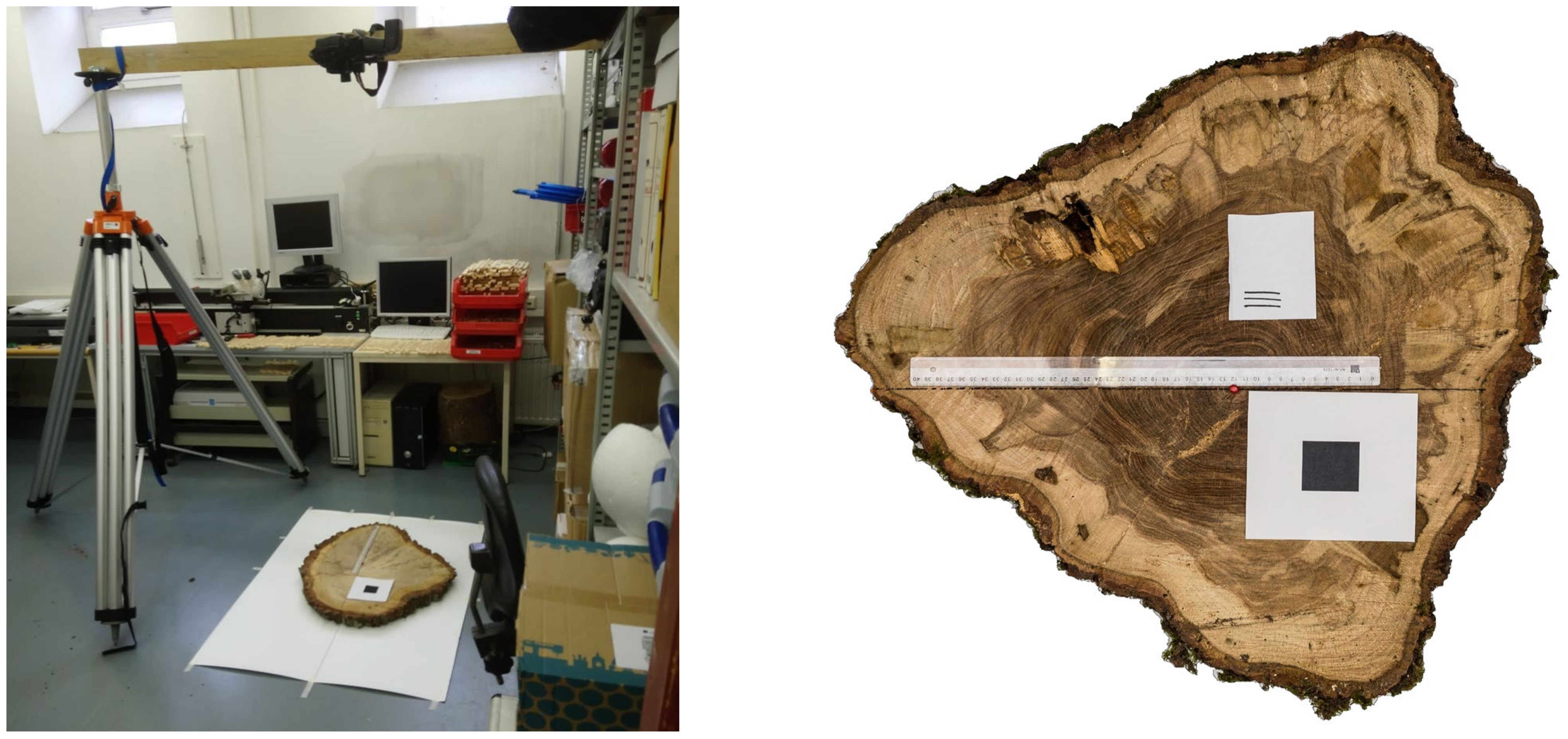
2.1. Study Area and Point Cloud Data Collection

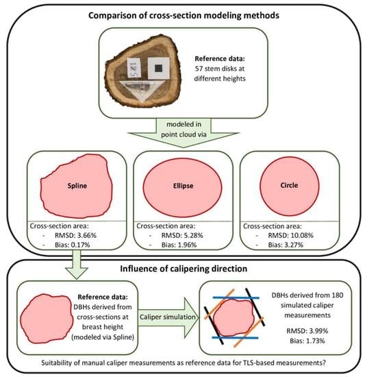
The workflow for data collection, presented in the following sections, is also clearly summarized in Appendix A.

The study site was located near Kattau, Lower Austria (48°41′N, 15°47′E). Laser scanning was conducted in February 2020 using a FARO Focus^3D X330 (Faro Technologies Inc., Lake Mary, FL, USA) terrestrial laser scanning system. The FARO Focus^3D X330 measures up to 976,000 points per second with a maximum range of 330 m using a wavelength of 1550 nm and providing an accuracy of ±2 mm per 10 m distance. For this study, the scanning parameters were set as described in Gollob et al. [12], with a quality parameter of 4× and a resolution of r = 6.136 mm/10 m.

In total, 20 sample trees were randomly selected from a pure sessile oak (Quercus petraea (Matt.) Liebl.) stand. Prior to the scans, breast height was indicated with paint mark spray, and the DBH of the standing trees were derived from crosswise measurements with a caliper at a height of 1.3 m above the ground. DBH measurements ranged from 22.5 to 44.5 cm, with an average of 34.65 cm and a standard deviation of 4.78 cm. Tree heights were measured with a Vertex IV Hypsometer (Haglöf AB, Långsele, Sweden); measurements ranged from 16.3 to 26.6 m, the average was 21.42 m and the standard deviation was 2.3 m. Tree diameters and heights were measured for descriptive purposes only and were not further used in the course of this study. All sample trees had an upright stem position, i.e., tilted stem orientations did not occur. Hence, the inclination was neglected for the DBH measurement.

Each individuum of the 20 total sample trees was scanned from at least three positions at approx. 10 m distance, to acquire complete point cloud data. Twelve white spheres with a diameter of 200 mm were positioned on tripods across the site to enable co-registration of the point cloud data of the multiple scans with the FARO SCENE 6.2 [25] software. As our study focus was on the analysis of the stem profiles, points that represented leaves, branches, underground vegetation, and soil were removed by using the CloudCompare 2.10.2 software [26].

2.2. Reference Data

To compare real-world and modeled cross-sections, the previously scanned sample trees were felled. From each of the felled sample trees, stem disks were cut from 2 to 4 different stem positions (depending on the tree height). This resulted in a total of 57 stem disks, which had thicknesses of 4–8 cm. For each of the stem disks, its position along the stem axis, its thickness, and two crosswise diameters were measured (

Table A2. Table with important parameters of the tree disks. The ratio of intersection and union represents the ratio that can be reached with the optimal parameter settings described in Section 3.1.

Tree Disk	Diameter 1 (cm)	Diameter 2 (cm)	Thickness (cm)	Height above the Ground (m)	Reference Area (cm²)	Area (cm2) Estimated Via			Ratio Intersection/Union (%)
						Spline	Ellipse	Circle	Spline	Ellipse	Circle
1_a	56	56	5	7	2786	2776	2926	2870	93.36	81.60	81.73
1_b	30	33	5	525	817	813	818	818	96.38	95.29	92.21
1_c	29	28	5	1044	661	660	666	671	94.89	95.02	95.38
1_d	21	21	5	1458	352	305	307	305	91.46	91.86	94.10
10_a	40	41	5	23	1393	1330	1355	1347	93.78	88.18	86.80
10_b	27	25	5	541	550	558	558	556	96.19	95.90	91.18
10_c	24	21	4	1052	422	411	420	415	94.33	92.30	88.06
11_a	45	41	5	11	1487	1461	1462	1488	94.70	93.66	90.31
11_b	32	30	5	331	753	750	750	751	96.33	95.72	94.45
11_c	29	28	4	646	643	640	635	632	93.56	92.69	93.09
12_a	46	59	6	10	2215	2158	2249	2370	89.99	83.06	82.60
12_b	33	32	6	333	869	904	905	903	95.65	94.84	93.62
13_a	35	37	5	22	1205	1167	1177	1173	95.12	94.36	93.67
13_b	26	25	4	340	532	533	534	533	95.70	95.39	94.57
13_c	22	22	4	653	382	393	400	394	94.30	94.24	95.57
13_d	17	18	4	964	258	240	238	239	91.72	90.47	91.53
14_a	36	37	5	8	1104	1095	1090	1077	94.26	91.96	89.61
14_b	26	29	5	337	581	582	582	577	97.24	96.55	91.97
15_a	54	46	5	12	2019	1990	2157	2242	93.87	84.12	85.21
15_b	35	33	5	340	987	965	965	960	95.42	95.93	93.27
15_c	32	32	4	637	813	819	817	816	96.54	96.21	96.12
15_d	28	29	4	940	669	668	672	672	96.67	96.95	96.43
16_a	41	44	5	9	1668	1648	1710	1766	92.52	91.60	88.19
16_b	33	33	5	332	876	882	883	881	96.78	96.92	95.25
16_c	31	31	5	636	767	754	761	762	93.63	94.82	94.11
17_a	39	42	6	21	1715	1759	1862	1842	90.15	75.23	77.38
17_b	31	30	5	343	738	711	710	712	92.62	93.79	93.43
17_c	29	27	4	658	620	647	647	647	94.52	93.67	93.09
18_a	51	52	5	17	2233	2252	2284	2273	95.47	90.20	90.76
18_b	34	35	8	344	935	928	929	932	96.45	96.44	96.27
18_c	33	31	5	659	843	833	836	840	96.10	95.37	93.88
19_a	68	56	6	18	2900	3029	2961	3215	92.13	85.70	79.64
19_b	37	36	5	290	1047	1009	1016	1019	96.96	95.91	95.96
20_a	67	63	5	10	2471	2462	2673	2750	82.84	73.88	76.95
20_b	35	33	5	331	890	903	905	897	92.79	92.94	93.39
21_a	57	50	5	7	2582	2770	2755	3190	85.74	86.05	85.10
21_b	33	31	6	321	856	823	824	826	96.36	95.88	94.04
21_c	31	27	5	639	684	710	713	713	95.36	94.61	91.34
22_a	42	46	5	28	1553	1569	1613	1589	92.61	84.21	83.70
22_b	30	28	5	344	674	687	689	692	95.35	94.16	92.85
22_c	27	27	4	660	575	560	558	558	96.41	95.52	95.62
22_d	34	34	5	974	476	478	504	486	85.29	85.84	87.73
3_a	37	32	5	15	1251	1240	1261	1280	91.77	88.56	85.33
3_b	21	23	4	537	416	395	394	391	86.87	79.90	85.02
3_c	20	19	4	1057	290	303	302	301	91.57	80.97	90.89
5_a	45	43	5	8	1116	1109	1228	1192	89.49	73.75	74.41
5_b	21	19	5	534	319	328	325	328	95.24	95.47	94.20
5_c	20	20	4	850	296	283	284	285	93.82	94.01	93.71
6_a	68	55	6	17	3031	3017	3058	3087	92.32	90.63	85.22
6_b	36	37	5	539	1115	1132	1147	1136	95.41	94.87	94.58
7_a	47	45	6	5	1765	1867	1869	1852	93.39	93.13	92.32
7_b	21	21	4	528	337	305	305	301	91.19	91.67	92.33
8_a	52	53	5	11	2327	2320	2355	2356	95.51	93.43	90.31
8_b	25	26	5	536	528	517	515	513	96.35	94.42	93.16
9_a	40	47	5	14	1966	2015	2032	1993	95.01	89.48	86.68
9_b	26	30	5	535	607	600	600	593	96.24	95.57	90.34

in Appendix A). The diameters had a range of 17.5–65.0 cm; the mean was 34.85 cm, and the standard deviation was 11.71 cm. These diameters were collected for descriptive purposes only and were not further used for the investigations regarding DBH caliper measurements, which are described in Section 2.6. The reference data for the latter were exclusively derived from the TLS point clouds since no real-life stem disks were taken at breast height.

One major objective of our analyses was to evaluate the in situ measurements of the TLS by means of in vitro measurements of the stem disks to quantify the influence of different cross-section modeling methods and parameter settings on the precision and accuracy of the cross-section area estimations with TLS. For this purpose, digital images of the stem disks were produced using a Canon EOS 6D camera (Canon Inc., Ōta, Tokyo, Japan) mounted on a scaffold 2 m above the stem slices, as shown in Figure 1. The surface of the stem disks was not enhanced by grinding or polishing prior to the taking of the photographs.

The plane of the camera sensor was aligned parallel to the floor using a Benro GD3WH geared head (Benro Precision Machinery Co., Ltd., Zhuhai, China) to avoid perspectival distortions. For the images of the larger stem disks, we used a Canon EF 50 mm f/1.8 STM lens, and for the smaller disks, we used a Canon EF 85 mm f/1.8 USM lens. We chose a wireless shutter release to avoid vibration. The image data were stored in the raw image file format. Exposure time (¹/₈₀ s), aperture (f/11), and sensor sensitivity (ISO400) were chosen manually. To achieve shadow-free illumination, exposure control was conducted with matrix metering and E-TTL bounce flash (Canon Speedlight 580 EX, Tokyo, Japan) against the ceiling. The RAW files were converted to JPEG files with a resolution of 5472 × 3648 pixels using Adobe Lightroom 5.7.1 (Adobe Inc., San José, CA, USA). The processing of the photos included white balance (5400 K), exposure adjustment (+1.21 EV), contrast enhancement (+20), and clarity (+50), as well as a lens distortion correction.

After the completion of these processing steps, the images as well as the outlines of the stem disks were cropped using a Magnetic Lasso tool in the image editing program PixBuilder Studio (WnSoft Ltd., Kirov, Russia, 2012). The cropped images were imported as tagged image files (TIFF) into the workspace of the R software (Version 3.6.3) [27] by using the stack command from the raster package [28]. A metric scale was placed along the stem disks during image collection. Hence, it was possible to calculate a geometric scaling factor for the raster images of the stem slices, using the functions zm [29] and locator [27]. The latter functions were also used to mark the center points of the cross-sections.

The images of the stem disk contour were likewise imported as TIFF files to extract the XY coordinates of the outer boundaries using the command xyFromCell [28]. The XY coordinates were transformed into polar coordinates using the center points as the origin.

To obtain continuous reference data, the circumference of stem disks was modeled with a cyclic cubic regression spline smoother and methodology implemented in the mgcv package [30]. For this purpose, the distances of the vertices to the center point were regressed against their azimuthal angle. The fitted models were subsequentially used to generate a set of predicted distances given a fine sequence of azimuthal angles in a 1° step width. The predicted polar coordinates were then transformed into Cartesian coordinates. The “true” reference area of the stem disks was calculated using the vertices of the smoothed circumference as outer boundary coordinates for polygon operation functionalities provided by the spatstat package [31].

2.3. Identification of Cross-Sections in the 3D TLS Point Clouds

To enable a comparison between the in vitro reference measurements of the stem disks and the in situ TLS measurements of the stem cross-sections, horizontal segments were extracted from the ground-based normalized point clouds at the position coordinates of the respective trees and at the height from where the stem disks were removed. Because the vertical width measurement of the stems disks in the field was tendentiously too small, and to consider the loss produced by the chainsaw kerf, we added an extra offset of 1 cm to the recorded upper and lower edges when we extracted the subsets from the point clouds. The exact position, orientation, and dimension of this subset in the point cloud were found via a grid search optimization (brute force algorithm). The contrast measure (minimum criterion) of the optimization was defined by the root mean squared deviation (RMSD) between 360 radius measurements from both the point cloud cross-sections and the corresponding in vitro stem disk measurements. The grid was spanned by four parameters: (i) the vertical height position with its set defined by the original height measurement and an offset of plus/minus 1 cm, the (ii) X and (iii) Y coordinates of the center point location that was iteratively shifted by a sequence of offsets ranging from −5 cm to 5 cm and having a step width of 2.5 cm, and (iv) the lateral rotation that was iteratively altered in 1° azimuthal steps. This approach produced a total number of 27,000 combinations of the position parameters. The initial starting point for the center point was derived via an ellipse fit using EllipseDirectFit from the conicfit package [32]. For each parameter combination, the circumference of the stem cross-section was modeled by a cyclic cubic regression spline smooth using the mgcv package. For a precise limitation of the optimal parameter combinations, the described grid search was conducted a second time by investigating only the 10 best parameter combinations, with the quality measure being the RMSD between the 360 radius measurements of the stem disk and the fitted circumference of the cross-section in the point cloud. In this second approach, the location parameters were no longer varied around an initial center derived via an ellipse fit, but around the initial center of the already-altered stem slice from the first level of this grid search.

The parameter combination that achieved the lowest RMSD was finally chosen to define the location and orientation of a point cloud subset that produces an optimal match with the outer boundary vertex coordinates of the collected stem disk. Once the optimum parameter configuration was found, the circumference of the cross-section was additionally modeled by using a cyclic cubic regression spline smooth, a circle fit, and an ellipse fit. The latter two fits were performed with the LMcircleFit and the EllipseDirectFit functions from the package conicfit [32].

The major goal of the analysis was to assess the precision and accuracy of the automatic stem cross-section modeling in 3D point clouds from TLS. For this purpose, the ratio of the intersection area and the union area of the geometries from both the stem disk and the cross-section modeling was used as a diagnostic measure. The geospatial computation was performed in R by using the gUnion and gIntersection functions from the rgeos [33] package.

2.4. Parameters of Cross-Section Modeling in the 3D TLS Point Clouds

Once the optimal position of the cross-section in the 3D TLS point cloud was determined by the procedure outlined above (Section 2.3), another optimization was conducted with respect to the modeling of the cross-section and to assess the optimal parameter combination of the cross-section models. Hence, we examined in detail the influence of the vertical cross-section width, the effect of data clustering prior to the cross-section modeling, and the number of knots of the smoothing splines, which was only applied to the spline fitting variant.

The optimization was performed via a grid search (brute force algorithm) across a large number of parameter combinations. The vertical cross-section width varied between 0.01 and 1 m in a step width of 0.01 m, the choice of clustering was binary (yes/no), and the tested number of knots of the spline bases was chosen from 5° to 245° in a 10° step width, resulting in 5000 possible parameter combinations for spline and 200 for circle and ellipse. Parameters of the cluster routines implemented in the optics and extractDBSCAN functions from the dbscan [34] package were fixed to constant values based on the results of preliminary experiments: eps_cl was set to 5, representing the threshold distance of two neighboring clusters; eps was set to 4.3; and minPts, the minimum number of points in a cluster, was set to 5. The contrast measure for this grid search was defined by the ratio of the intersection area and the union area of the cross-sections and the stem disks, i.e., the final performance criterion of the automatic measurement routines.

2.5. Comparison of the Different Cross-Section Modeling Methods

Once the optimal parameter combinations for the three different cross-section modeling methods were determined by the procedure outlined above (Section 2.4), the cross-section models with the optimal parameter combinations were selected and compared for all stem slices.

Precision and accuracy of the three investigated cross-section modeling methods were assessed in terms of estimated percentual RMSD (Equation (1)) and percentual estimated bias (Equation (2)), with ${\widehat{y}}_i$ being the modeled cross-section area of the ith stem disk, $y_i$ being the reference cross-section area of the ith stem disk, and $\overline{y}$ being the mean reference cross-section area of all $n=57$ stem disks.

$$RMSD\%=\frac{100}{\overline{y} }\sqrt{\frac{1}{n}{{\displaystyle \sum }}_{i=1}^n{\left({\widehat{y}}_i-y_i\right)}^2}$$

(1)

$$bias\%=\frac{100}{\overline{y}}\frac{1}{n} {{\displaystyle \sum }}_{i=1}^n\left({\widehat{y}}_i-y_i\right)$$

(2)

A repeated-measures ANOVA with Greenhouse-Geisser sphericity correction was performed to assess the statistical significance of the observed differences between cross-section areas, modeled by the different methods and the reference cross-section areas. Post hoc pairwise comparisons were performed using Holm corrected pairwise paired t-tests.

2.6. Calipering Direction and Accuracy

To analyze the influence of the caliper direction on the accuracy of the manual DBH measurement and its further propagation to the volume estimates, extra cross-sections of 2 cm thickness were cropped at 1.3 m breast height from the TLS point clouds. The geometry of these cross-sections was modeled using cyclic cubic regression splines with the optimum parameter settings derived from Section 2.4. Under the assumption of a circular cross-section, the reference diameter at breast height DBH* was calculated via $2\sqrt{\frac{are{a}_{ref}}{\pi }}$, with $are{a}_{ref}$ being the area estimate of the stem disk modeled by a regression spline smoother. The methodology for modeling with this regression spline smoother was the same as described in Section 2.2. Moreover, DBH measurements were simulated using the modeled cross-section areas for iteratively changed caliper directions from 0° to 179° in a 1° step width. These simulated caliper DBH measurements were then compared with DBH* to analyze the effect of circular assumptions on the DBH estimate. Precision and accuracy of the simulated caliper measurements were assessed in terms of estimated percentual RMSD (Equation (1)) and percentual estimated bias (Equation (2)), with ${\widehat{y}}_i$ being the ith simulated DBH measurement, $y_i$ being the ith DBH*, $\overline{y}$ being the mean DBH* and $n=3600$ being the number of simulated caliper measurements (20 trees and 180 measurements per tree). The cross-section areas derived from the TLS data (as described in Section 2.4) were thus used as reference data for the simulated caliper measurements. The histograms in Appendix B show the distribution of 180 simulated DBH measurements for each tree separately. Cross-calipering was simulated by tree-wise calculating the arithmetic, quadratic, and geometric mean of the minimum and maximum DBH value obtained from the 180 simulated caliper measurement directions.

A repeated-measures ANOVA with Greenhouse-Geisser sphericity correction was performed to assess the statistical significance of the observed differences between the DBH estimates from simulated cross-calipering and DBH*. Post hoc pairwise comparisons were performed using Holm corrected pairwise paired t-tests.

3. Results

3.1. Optimization of Parameters for Cross-Section Modeling

As described in Section 2.4, we analyzed the ratio of the intersection and the union area between the cross-sections of the stem disks and their counterparts extracted from the point cloud in terms of different parameter combinations (slice thickness, clustering, number of knots for spline). The best match, i.e., the highest ratio, was obtained by a prior clustering of the data and by using a slice thickness of 2 cm. This setting proved to be the best solution for all three cross-section modeling methods. The maximum ratio achieved with an ellipse fit was 91.27% and 89.57% with a circle fit. The spline regression achieved a ratio of 94.05% with an optimum number of 95 knots. However, we found that the accuracy of the spline regression did not significantly change when we tested different numbers of knots. With 125 knots, the spline regression produced a ratio of 94.01%, and with 35 knots, the ratio became 94.00%. Hence, choosing the thickness of the extracted slice and the clustering was more important than the number of knots.

When we analyzed the effect of the different cross-section thicknesses that were extracted from the point cloud, we found that the ratio of the intersection area and the union area decreases with an increasing thickness beyond the optimum of 2 cm (Figure 2). Slices thinner than 2 cm proved to be unfavorable because the number of included points was simply too small to enable an accurate model fit of the outer circumference.

When the number of knots was automatically determined by the statistical methodology implemented in mgcv, useful results were produced in terms of a relatively high ratio of the intersection area and the union area. However, the maximum possible ratio was obtained with a predefined number of 95 knots for the regression splines. With an increased thickness of the cross-sections, the difference became smaller between the ratio values obtained by the automatic knot selection and by a fixed number of 95 basis spline knots.

The results showed that clustering, which was conducted to remove possible outliers, was generally favorable, especially for a cross-section thinner than 60 cm. For wider cross-sections, clustering had only a small effect (Figure 2). In addition, we found that clustering had only minor relevance for the spline regression method, whereas the ratios of the intersection areas obtained from the ellipse and the circle fitting methods could be enhanced through clustering by approximately 3% and 1%, respectively.

In addition to the ratio of the intersection and the union area, the parameter selection was also assessed by means of the relative difference between the modeled cross-section areas of the stem disks and the point clouds (Figure 3). To calculate this quality measure, the difference between the modeled and reference cross-section areas was divided through the reference cross-section area. We found that the difference was generally lower for thinner cross-sections from the point cloud, i.e., the modeled cross-section area from the point clouds approached the modeled area of the stem disk for thinner slices. However, the differences showed a distinct maximum around slice thicknesses between 0.4 and 0.5 m for the spline and the ellipse model fits. In addition, we found that the difference was generally lowered by a prior clustering of the point cloud.

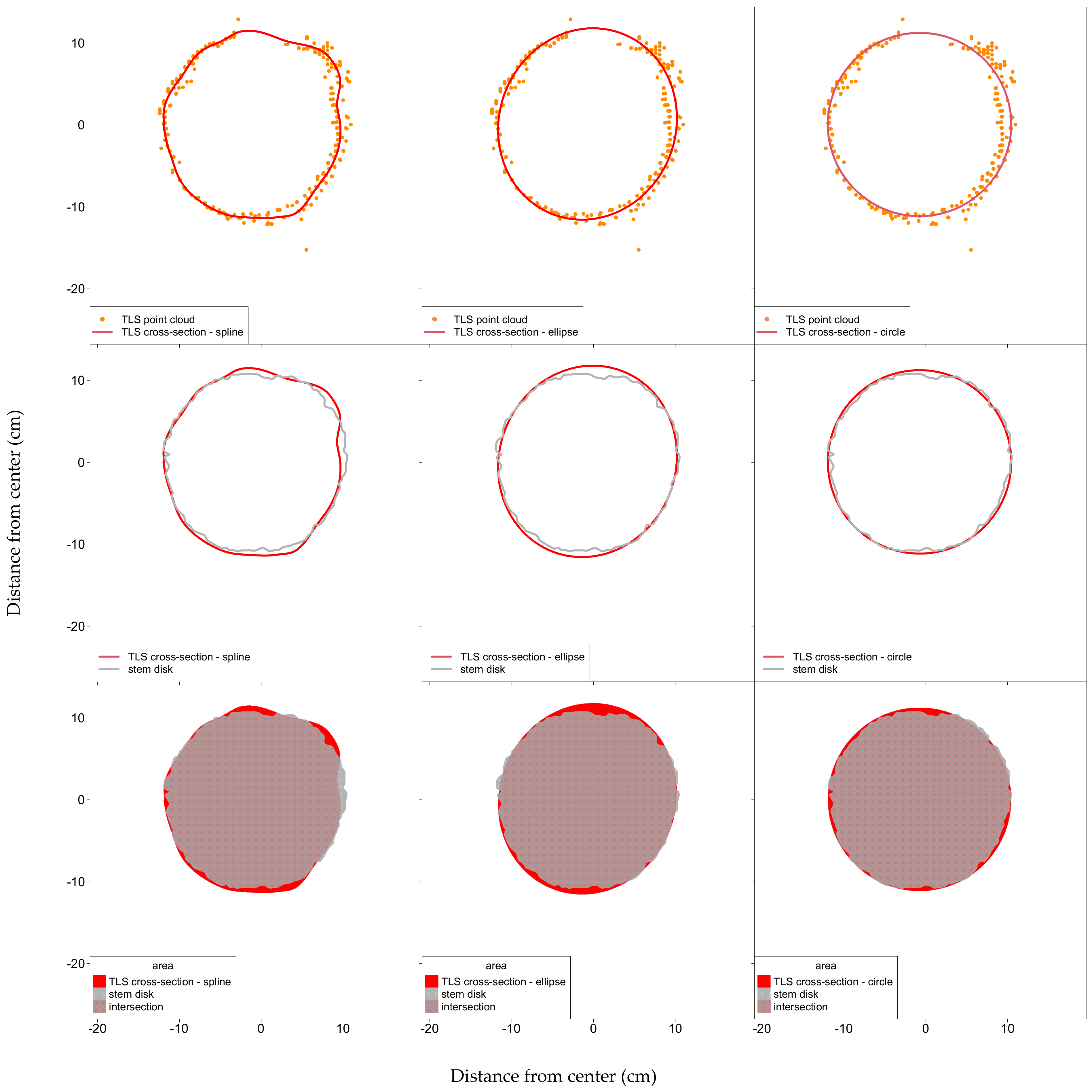
3.2. Comparison of Cross-Section Modeling Methods

3.2.1. Effect of Parameter Selection

The ratio of the intersection area and the union area between the modeled cross-sections from the point clouds and the stem disks was also analyzed to compare the spline, ellipse, and circle fit techniques for the modeling of the stem slice shape (Figure 4). Across all 5000 possible parameter combinations, the ratio of the intersection and the union area was on average 88.69% and ranged from 84.14% to 94.05% with the spline approach. The ellipse fit achieved an average ratio of 84.46% across all 200 possible parameter combinations and the range was 80.03% to 91.27%. The circle fit ratios had an average of 86.54% and ranged from 84.05% to 89.57%. The circle fit method was relatively robust for a wide range of different parameter combinations.

3.2.2. Comparison of the Different Models with Optimal Parameter Combination

As demonstrated on a cross-section extracted from a 14 cm stem height (Figure 5), the spline approach is flexible and can also represent irregular stem circumferences. This is contrary to the ellipse and circle fitting techniques, which both simply failed in this situation.

However, the ellipse and the circle fit have also produced accurate results, especially for cross-sections that were extracted from higher stem positions and had a more regular shape. For example, this was the case for stem slices such as the one depicted in Figure 6, which was taken at a stem height of 6.57 m. The height above the ground along with the ratio of intersection and union for each investigated stem disk can be derived from Table A2 in Appendix A.

The different accuracies of the three investigated modeling methods were also assessed by comparing the percentual RMSD and the percentual bias of the modeled cross-section areas, as described in Section 2.5. Figure 7 shows the results of these calculations. The percentual RMSD values were 3.657%, 5.275% and 10.075% for spline, ellipse, and circle fitting, respectively. The percentual bias was 0.173% for spline fitting, 1.963% for ellipse fitting, and 3.266% for circle fitting. The coefficient of determination R² was quite high for all three cross-section models, ranging from 0.991 for circle to 0.997 for spline and ellipse. Note that the ellipse performed better in Figure 7 than in Figure 4 because the cross-section areas in Figure 7 were derived solely from the cross-sections modeled with the parameter settings from Section 3.1 and clustering was conducted, whereas Figure 4 analyzes the performance of the three modeling methods for all possible parameter combinations.

The repeated-measures ANOVA indicated significant differences (p = 0.005) between the cross-section areas obtained by the different modeling approaches and the reference. Holm corrected pairwise paired t-tests indicated no significant difference between the spline and the reference (p = 0.725), but significant differences between circle and reference (p = 0.039) and ellipse and reference (p = 0.016) (Figure 8).

3.3. Influence of Caliper Orientation

The influence of the caliper orientation on the diameter estimation was examined as outlined in Section 2.6. The applied method allowed for a detailed comparison of the DBH estimates obtained from the simulated caliper measurements with the reference DBH* obtained from the TLS data via spline fitting. DBH* was used as ground truth because it can be assessed non-destructively and because the spline fit showed no significant difference to the reference data in Section 3.2. The average coefficient of variation (standard deviation divided through DBH*) of the simulated DBH measurements of a single tree was 3.22% and ranged from 1.44% to 5.84% (Figure 9).

On average and across all trees, the ideal DBH* lay at the 34th percentile of the simulated DBH measurements (Figure 10). Hence, 66% of the caliper DBH measurements led to an overestimation of the true cross-section area. The bias of the DBH measurements was 0.596 cm (Figure 11), corresponding to a percentual bias of 1.726%. The percentual RMSD of the DBH measurements was 3.985%.

Stem volume estimation is usually based on the assumption of a circular cross-section area. Thus, the estimated stem volume and basal area increase geometrically with increasing DBH. Overestimating DBH by 1.726% would thus result in an overestimation of the cross-section area and volume of 3.482%.

The repeated-measures ANOVA indicated significant differences (p < 0.0001) between the DBH values obtained from simulated cross-calipering and DBH*. Holm corrected pairwise paired t-tests indicated a significant difference between DBH* and all simulated cross-calipering estimates (p < 0.0001) (Figure 12).

4. Discussion

4.1. Optimization of Parameters for Cross-Section Modeling

A sufficient point cloud density is crucial when geometric shapes are modeled from TLS data. In our study, a slice thickness of 2 cm produced the best results for the cross-section modeling. However, the point cloud density was relatively high in our study because each tree was scanned from three positions that had a close distance to the trees.

As indicated by Liu et al. [8], thinner stem disks might also enable precise modeling if the point cloud density is sufficiently high, whereas an increasing thickness of the stem disks could rather increase the number of outliers and produce more noise. In general, it is recommended to use thinner cross-sections with higher point densities. This was also demonstrated in Srinivasan et al. [19], who chose a slice thickness of 10 and 20 cm to retrieve the DBH from high-density TLS point cloud data acquired in the multi-scan mode, and when slice thickness was increased up to 60 cm for single-scan data. These results were also in accordance with the findings of Liu et al. [8], who suggested using larger height bins for the single-scan mode and smaller height bins for the multi-scan mode.

However, the choice of a thicker cross-section might also be favorable as it can reduce the cross-section height error, which likely occurs due to inaccuracies of the DTM and the stem base estimation [19]. This effect could explain the maximum deviation of the cross-section area in Figure 3. Below a threshold of 40–50 cm slice thickness, the deviation might have increased through the increasing influence of outliers. Beyond this threshold, the effect of a reduction in the cross-section height error might have outweighed the error introduced by an increasing number of outliers.

Another explanation for the latter phenomenon might be the increasing number of points in general, which was associated with a tendentiously stronger increase in evaluable points than in outlying points. Likewise, this large increase in the number of evaluable points might have compensated for the effects produced by the outliers, eventually leading to lower deviations from the true cross-section area. This approach would also explain why the positive impact of clustering on the accuracy of cross-section modeling was only noticeable for a slice thickness below 60 cm (Figure 2), as the impact of outliers decreases with an increasing slice thickness. The small difference between the modeling methods with and without clustering above the threshold of 60 cm could thus be the result of the decreasing influence of outliers for a slice thickness larger than 60 cm. Clustering, however, is in most cases a crucial component of data preprocessing [18].

As described by Wang et al. [20], the influence of slice thickness on the results of DBH estimation largely depends on the angular step width. The authors found that the accuracy of DBH estimation was generally enhanced with increasing slice thickness, but this finding only held for larger angular step widths. However, smaller angular step widths generally resulted in a sufficient number of points, making an additional increase in the point number through an increased slice thickness unnecessary. The authors thus hypothesized that the angular step width had a greater impact on DBH estimation than the slice thickness. Nevertheless, slice thickness is considered an important parameter for cross-section modeling in many studies [8,19,21].

Another important modeling parameter relevant for spline fitting is the knot number. Pfeifer and Winterhalder [35], for example, noted the importance of knot number for spline modeling: a greater number of knots allows for a precise approximation of the stem profile, whereas a restricted knot number provides a smooth spline curve fit and prevents greater “wiggliness” through outliers. For the identification of the ideal knot number for spline fitting, Pfeifer and Winterhalder [35] suggested a method for sequentially inserting knots, which is, however, time- and computation-intensive. In fact, our results suggest that the slice thickness and the clustering have greater impacts on the spline modeling than the knot number. The five best solutions of the parameter settings had a slice thickness of 2 cm combined with clustering, whereas a varying knot number had only a minor influence. As demonstrated in Figure 2, the ratio of the intersection and union area did not differ much between the different solutions varying in the number of knots.

4.2. Comparison of Cross-Section Modeling Methods

In our study, the regression spline method generally showed the best performance in the modeling of the stem cross-sections and achieved the highest ratios of the intersection and union area (84.14–94.05%) and the lowest bias for cross-section area estimation (0.173%). The post hoc pairwise comparisons of the repeated-measures ANOVA indicated significant differences between the cross-section area estimates obtained by circle and ellipse fit and the reference, whereas no significant differences were found between the estimates obtained by spline fit and the reference. The superiority of the spline fits over simpler modeling techniques was likewise confirmed in other studies [18,36]. You et al. [18] noted that more flexible cross-section modeling methods, such as convex hull line fitting, closure Bézier curve, or B-spline fitting, can consider irregular shapes of the cross-sections. However, these approaches have disadvantages, as well—implementation is not always straightforward and reliable fits require a higher point cloud density. Therefore, circle or cylinder fitting algorithms might be also recommended, especially if the completeness of the stem point cloud is below a certain threshold [18]. Outliers and a heterogeneous point cloud density around the stem cross-section are common sources of error, which might produce illogical curve fits [35].

The ratio of the intersection and union area showed a wider range and a higher variance with the ellipse fitting approach than with the other two methods (Figure 4). For the majority of the examined stems, the spline regression performed better than the ellipse fit. This was especially because the ellipse fit was more sensitive to outliers (see results without clustering in Figure 3). Our results correspond well with similar findings by Åkerblom et al. [13], who used circular as well as elliptical cones for stem reconstructions and noted a larger instability for the latter approach compared to the other modeling methods.

Ritter et al. [11] stated that an ellipse fit might be superior to a circle fit. In our study, the ellipse fitting results were, depending on the parameter combinations, able to achieve higher ratios of intersection-to-union compared to the circle fitting method. The average ratio achieved with a circle fit, however, was higher than that of the ellipse fit. This finding emphasizes the higher robustness of a circle fit that was further confirmed by the tight range of ratios achieved with circle fitting (84.05% to 89.57%). Similar results were derived in the study of Åkerblom et al. [13], in that the circular cones proved to be the more robust in terms of data quality and modeling parameter settings when compared with elliptical cones and other, more complex approaches. Nevertheless, the cross-section areas estimated via ellipse fits exhibited a lower percentual bias (1.963%) than the area estimates from circle fitting (3.266%). The percentual RMSD of the latter was also relatively high (10.075%) compared to the percentual RMSD of the cross-section areas from ellipse fitting (5.275%). When analyzing the differences between these values and the modeling methods in Figure 7, it becomes obvious that especially for the larger, more eccentric stem cross-sections, the additional flexibility provided by ellipse fitting is an advantage. However, as mentioned before, clustering and outlier removal are crucial factors for obtaining accurate results from ellipse fitting.

Another important factor that influences the cross-section modeling is the height from which the cross-section was extracted. As demonstrated in Figure 5 and Figure 6, the accuracy of the chosen model technique is strongly dependent on the shape of the cross-section’s circumference. Similar to what we had expected, cross-sections from an upper part of the stem had nearly circular shapes, whereas those from the lower trunk often had irregular shapes. Thus, a circle fit provided accurate results for the upper cross-sections, and a regression spline fit was better suited for the lower stem. Our results correspond well with Hunčaga et al. [5], who found that circle fits produced a larger RMSE of the diameter estimation on cross-sections from lower stem parts. Accordingly, the bias of the cross-section areas estimated via circle fitting in Figure 7 is larger for large cross-sections that were taken from lower stem parts.

4.3. Influence of Caliper Orientation

The problems and inaccuracies that eccentric cross-sections may produce in forest mensuration when manual caliper measurements are used have already been discussed in the literature [2,37]. For the estimation of basal area and stem volume from caliper diameter measurements, a circular cross-section area is traditionally assumed. However, perfectly circular cross-sections rarely occur in practice. In particular, the lower parts of the stem usually have an undulating contour, which has a major influence on the diameter measurement using calipers [5,23].

Similar to the approach in our study, You et al. [18] examined caliper measurements on simulated convex hulls. The ovality, i.e., the ratio of the minimum and the maximum diameter, of the simulated cross-sections ranged from 2.60% to 49.30% and was on average 8.80%. These values indicate a high potential for errors in the diameter and thus volume estimation by manual caliper measurements, corresponding well with our findings. The oaks in our study exhibited highly eccentric contours in lower stem parts, resulting in possible volume estimation errors of up to 20% because of stem eccentricity.

Our results showed that caliper diameter measurements together with circular basal area assumptions produce a systematic overestimation of the stem volume compared with the reference cross-sections. This was because in 66% of the cases, the simulated caliper DBH measurements were larger than those derived from the regression spline fit (Figure 10). The percentual bias of the simulated caliper DBH measurements was 1.726%, with a percentual RMSD of 3.985% (Figure 11). Cross-calipered diameters also exhibited significant differences to the reference DBH*, with highly significant differences occurring between different averaging methods as well (arithmetic, quadratic, and geometric mean) (Figure 12). This corresponds with the findings of Smaltschinski [24], who investigated the same averaging methods for cross-calipering and discovered a high potential for cross-section area estimation errors.

Regarding these facts, the common approach of assessing the accuracy of TLS-based DBH estimates by comparing them with caliper measurements (ground truth) becomes questionable. At least for our data, TLS was more accurate and precise than the caliper measurements, and using ground truth that is less exact than the remotely sensed data is paradoxical.

Besides the more accurate single-tree basal area measurement, TLS can also provide additional measurements at other locations from upper parts along the stem axis. Hence, the broader application of terrestrial laser-scanning technology in future forest inventory applications will contribute to enhanced accuracy of the growing stock volume estimates, in general.

5. Conclusions

In this study, we compared circle, ellipse and spline fits as possible cross-section modeling methods. After an optimization of the parameters—possible clustering, the slice thickness, and the number of basis spline knots (only applied to the spline method)—the best performance was achieved by the spline method. Although the cross-section modeling via regression splines provided the closest congruence with the cross-sections of stem disks extracted from the felled trees (bias% = 0.173%), the spline method was sensitive to the parameter settings. In contrast, the circle and ellipse fits were less sensitive to parameter settings that differed from the optimum solution. Because of this fact and due to their easy implementation, circle and ellipse fits can be regarded as highly efficient, especially when applied to cross-sections that have a nearly regular shape. However, with modern computer facilities and the high completeness and density of TLS point cloud data, we generally recommend the regression spline method as a standard technique for cross-section modeling. As a drawback, the regression spline technique requires a more careful adjustment of parameters depending on the point cloud density and the quality of the acquired data.

Because of the high accuracy of the spline technique, it was further used to study the influence of stem eccentricity and caliper orientation on the accuracy of the cross-section area estimation by means of manual diameter measurements with traditional calipers. Our simulation study showed that manual calipering leads to a systematic overestimation of the stand volume, with the corresponding bias% = 1.726% (Figure 11). Moreover, 66% of all measurable diameters were larger than the “perfect” diameter (Figure 10).

At least for our data, TLS-based estimates have reached an accuracy level surpassing traditional caliper measures. Thus, further usage of caliper measures as ground truth for TLS-based estimates becomes paradoxical if TLS data quality is high enough to obtain reliable spline fits.

References

1. Kershaw, J.A.; Ducey, M.J.; Beers, T.W.; Husch, B. Forest Mensuration, 5th ed.; John Wiley & Sons, Ltd.: Chichester, UK, 2016; ISBN 9781118902028. [Google Scholar]
2. Tischendorf, W. Der Einfluss Der Exzentrizität der Schaftquerflächen Auf Das Messungsergebnis Bei Bestandesmassenermittlungen Durch Kluppung. Cent. Gesamte Forstwes. 1943, 69, 87–94. [Google Scholar]
3. Liang, X.; Kankare, V.; Hyyppä, J.; Wang, Y.; Kukko, A.; Haggrén, H.; Yu, X.; Kaartinen, H.; Jaakkola, A.; Guan, F.; et al. Terrestrial Laser Scanning in Forest Inventories. ISPRS J. Photogramm. Remote Sens. 2016, 115, 63–77. [Google Scholar] [CrossRef]
4. Panagiotidis, D.; Abdollahnejad, A. Accuracy Assessment of Total Stem Volume Using Close-Range Sensing: Advances in Precision Forestry. Forests 2021, 12, 717. [Google Scholar] [CrossRef]
5. Hunčaga, M.; Chudá, J.; Tomaštík, J.; Slámová, M.; Koreň, M.; Chudý, F. The Comparison of Stem Curve Accuracy Determined from Point Clouds Acquired by Different Terrestrial Remote Sensing Methods. Remote Sens. 2020, 12, 2739. [Google Scholar] [CrossRef]
6. Olofsson, K.; Holmgren, J.; Olsson, H. Tree Stem and Height Measurements Using Terrestrial Laser Scanning and the RANSAC Algorithm. Remote Sens. 2014, 6, 4323–4344. [Google Scholar] [CrossRef] [Green Version]
7. Pueschel, P.; Newnham, G.; Rock, G.; Udelhoven, T.; Werner, W.; Hill, J. The Influence of Scan Mode and Circle Fitting on Tree Stem Detection, Stem Diameter and Volume Extraction from Terrestrial Laser Scans. ISPRS J. Photogramm. Remote Sens. 2013, 77, 44–56. [Google Scholar] [CrossRef]
8. Liu, C.; Xing, Y.; Duanmu, J.; Tian, X. Evaluating Different Methods for Estimating Diameter at Breast Height from Terrestrial Laser Scanning. Remote Sens. 2018, 10, 513. [Google Scholar] [CrossRef] [Green Version]
9. Heinzel, J.; Huber, M.O. Tree Stem Diameter Estimation from Volumetric TLS Image Data. Remote Sens. 2017, 9, 614. [Google Scholar] [CrossRef] [Green Version]
10. Bu, G.; Wang, P. Adaptive Circle-Ellipse Fitting Method for Estimating Tree Diameter Based on Single Terrestrial Laser Scanning. J. Appl. Remote Sens. 2016, 10, 026040. [Google Scholar] [CrossRef]
11. Ritter, T.; Schwarz, M.; Tockner, A.; Leisch, F.; Nothdurft, A. Automatic Mapping of Forest Stands Based on Three-Dimensional Point Clouds Derived from Terrestrial Laser-Scanning. Forests 2017, 8, 265. [Google Scholar] [CrossRef]
12. Gollob, C.; Ritter, T.; Wassermann, C.; Nothdurft, A. Influence of Scanner Position and Plot Size on the Accuracy of Tree Detection and Diameter Estimation Using Terrestrial Laser Scanning on Forest Inventory Plots. Remote Sens. 2019, 11, 1602. [Google Scholar] [CrossRef] [Green Version]
13. Åkerblom, M.; Raumonen, P.; Kaasalainen, M.; Casella, E. Analysis of Geometric Primitives in Quantitative Structure Models of Tree Stems. Remote Sens. 2015, 7, 4581–4603. [Google Scholar] [CrossRef] [Green Version]
14. Wang, D.; Hollaus, M.; Puttonen, E.; Pfeifer, N. Fast and robust stem reconstruction in complex environments using terrestrial laser scanning. In Proceedings of the International Archives of the Photogrammetry, Remote Sensing and Spatial Information Sciences—ISPRS Archives; International Society for Photogrammetry and Remote Sensing, Prague, Czech Republic, 12–19 July 2016; Volume 41, pp. 411–417. [Google Scholar]
15. Thies, M.; Pfeifer, N.; Winterhalder, D.; Gorte, B.G.H. Three-Dimensional Reconstruction of Stems for Assessment of Taper, Sweep and Lean Based on Laser Scanning of Standing Trees. Scand. J. For. Res. 2004, 19, 571–581. [Google Scholar] [CrossRef]
16. Puletti, N.; Grotti, M.; Scotti, R. Evaluating the Eccentricities of Poplar Stem Profiles with Terrestrial Laser Scanning. Forests 2019, 10, 239. [Google Scholar] [CrossRef] [Green Version]
17. Sun, H.; Wang, G.; Lin, H.; Li, J.; Zhang, H.; Ju, H. Retrieval and Accuracy Assessment of Tree and Stand Parameters for Chinese Fir Plantation Using Terrestrial Laser Scanning. IEEE Geosci. Remote Sens. Lett. 2015, 12, 1993–1997. [Google Scholar] [CrossRef]
18. You, L.; Wei, J.; Liang, X.; Lou, M.; Pang, Y.; Song, X. Comparison of Numerical Calculation Methods for Stem Diameter Retrieval Using Terrestrial Laser Data. Remote Sens. 2021, 13, 1780. [Google Scholar] [CrossRef]
19. Srinivasan, S.; Popescu, S.C.; Eriksson, M.; Sheridan, R.D.; Ku, N.W. Terrestrial Laser Scanning as an Effective Tool to Retrieve Tree Level Height, Crown Width, and Stem Diameter. Remote Sens. 2015, 7, 1877–1896. [Google Scholar] [CrossRef] [Green Version]
20. Wang, P.; Gan, X.; Zhang, Q.; Bu, G.; Li, L.; Xu, X.; Li, Y.; Liu, Z.; Xiao, X. Analysis of Parameters for the Accurate and Fast Estimation of Tree Diameter at Breast Height Based on Simulated Point Cloud. Remote Sens. 2019, 11, 2707. [Google Scholar] [CrossRef] [Green Version]
21. Koreň, M.; Hunčaga, M.; Chudá, J.; Mokroš, M.; Surový, P. The Influence of Cross-Section Thickness on Diameter at Breast Height Estimation from Point Cloud. ISPRS Int. J. Geo-Inf. 2020, 9, 495. [Google Scholar] [CrossRef]
22. Tong, Q.J.; Zhang, S.Y. Stem Form Variations in the Natural Stands of Major Commercial Softwoods in Eastern Canada. For. Ecol. Manag. 2008, 256, 1303–1310. [Google Scholar] [CrossRef]
23. Matérn, B. On the Geometry of the Cross-Section of a Stem; Statens Skogsforskningsinstitut: Stockholm, Sweden, 1956. [Google Scholar]
24. Smaltschinski, T. Fehler Bei Stammscheiben-Und Bohrspananalysen. Forstwiss. Cent. 1986, 105, 163–171. [Google Scholar] [CrossRef]
25. FARO Technologies FARO SCENE. Available online: https://www.faro.com/en/Products/Software/SCENE-Software/ (accessed on 23 February 2019).
26. Girardeau-Montaut, D.C. 3D Point Cloud and Mesh Processing Software. 2017. Available online: https://www.cloudcompare.org/ (accessed on 25 February 2020).
27. R Core Team. R: A Language and Environment for Statistical Computing. 2020. Available online: https://www.r-project.org/ (accessed on 20 December 2019).
28. Hijmans, R.J. Raster: Geographic Data Analysis and Modeling. 2020. Available online: https://cran.r-project.org/web/packages/raster/index.html/ (accessed on 11 March 2020).
29. Barbu, C.M. Zoom: A Spatial Data Visualization Tool. 2013. Available online: https://cran.r-project.org/web/packages/zoom/index.html/ (accessed on 20 February 2020).
30. Wood, S.N. Generalized Additive Models: An Introduction with R, 2nd ed.; Chapman and Hall/CRC: London, UK, 2017. [Google Scholar]
31. Baddeley, A.; Turner, R. Spatstat: An R Package for Analyzing Spatial Point Patterns. J. Stat. Softw. 2005, 12, 1–42. [Google Scholar] [CrossRef] [Green Version]
32. Gama, J.; Chernov, N. Conicfit: Algorithms for Fitting Circles, Ellipses and Conics Based on the Work by Prof. Nikolai Chernov. 2015. Available online: https://cran.r-project.org/web/packages/conicfit/index.html/ (accessed on 29 February 2020).
33. Bivand, R.; Rundel, C. Rgeos: Interface to Geometry Engine—Open Source (‘GEOS’). 2020. Available online: https://cran.r-project.org/web/packages/rgeos/index.html/ (accessed on 3 March 2020).
34. Hahsler, M.; Piekenbrock, M.; Doran, D. Dbscan: Fast Density-Based Clustering with R. J. Stat. Softw. 2019, 91, 1–30. [Google Scholar] [CrossRef] [Green Version]
35. Pfeifer, N.; Winterhalder, D. Modelling of Tree Cross Sections from Terrestrial Laser Scanning Data with Free-Form Curves. Int. Arch. Photogramm. Remote Sens. Spat. Inf. Sci. 2004, 36 Pt 8, W2. [Google Scholar]
36. Hong’e, R.; Yan, W.U.; Zhu, X.-M. The Quadratic B-Spline Curve Fitting for the Shape of Log Cross Sections. J. For. Res. 2006, 17, 150–152. [Google Scholar]
37. Graves, H.S. Forest Mensuration, 1st ed.; John Wiley & Sons: New York, NJ, USA, 1906. [Google Scholar]
Figure 1. Configuration of scaffold for photographing, and photo of an exemplary stem slice (slice_id = 3).
Remotesensing 14 01923 g001
Figure 2. Ratio of intersection and union between modeled and reference cross-section areas depending on slice thickness, clustering, and knot number.
Remotesensing 14 01923 g002
Figure 3. Relative difference of modeled and reference cross-section areas depending on slice thickness, clustering, and knot number.
Remotesensing 14 01923 g003
Figure 4. Ratio of intersection and union for the 3 modeling methods over all investigated parameter combinations for cross-section modeling.
Remotesensing 14 01923 g004
Figure 5. Comparison of the ratios of intersection and union between reference and modeled cross-section areas for an exemplarily irregular stem cross-section and 3 modeling methods. The illustrations for spline, ellipse, and circle (red) are depicted column-wise, in that order. In the first row, the point cloud of the TLS stem slice to which the cross-section model has been fitted is shown in a transparent red. This cross-section model is further compared with the outline of the photographed reference stem slice (gray) in the second row. In the third row, the difference between the areas of modeled (red) and reference (gray) cross-sections as well as the intersection of these two (reddish gray) are depicted. The ratio of intersection and union was 94.77% for spline fitting, 81.59% for ellipse fitting and 81.69% for circle fitting.
Remotesensing 14 01923 g005
Figure 6. Comparison of the ratios of intersection and union between reference and modeled cross-section areas for an exemplarily regular stem cross-section and 3 modeling methods. The ratio of intersection and union was 93.46% for spline fitting, 93.72% for ellipse fitting and 95.52% for circle fitting.
Remotesensing 14 01923 g006
Figure 7. Modeled spline, ellipse, and circle cross-section areas compared to reference cross-section areas; the reference line is the 1:1 line.
Remotesensing 14 01923 g007
Figure 8. Visualization of the pairwise paired t-tests for the cross-section models. ns and * indicate significance for type-one-error probabilities of p ≥ 0.05 and p < 0.05, respectively.
Remotesensing 14 01923 g008
Figure 9. Distribution of the coefficient of variation of the simulated DBH measurements per tree.
Remotesensing 14 01923 g009
Figure 10. Quantiles of the ideal DBH* measurements within the distributions of the simulated caliper measurements.
Remotesensing 14 01923 g010
Figure 11. Comparison of the diameters from the caliper simulation (DBH) and the diameters derived from the real cross-section area (DBH*). For every tree, there is one DBH* and 180 DBHs.
Remotesensing 14 01923 g011
Figure 12. Visualization of the pairwise paired t-test for the DBH estimates. **** indicate significance for type-one-error probability of p < 0.0001.
Remotesensing 14 01923 g012
Publisher’s Note: MDPI stays neutral with regard to jurisdictional claims in published maps and institutional affiliations.