
Semi-Automated Mapping of Complex-Terrain Mountain Glaciers by Integrating L-Band SAR Amplitude and Interferometric Coherence

 ,
, 
 , ,
, ,  and
and
Abstract
:1. Introduction
2. Study Area and Dataset
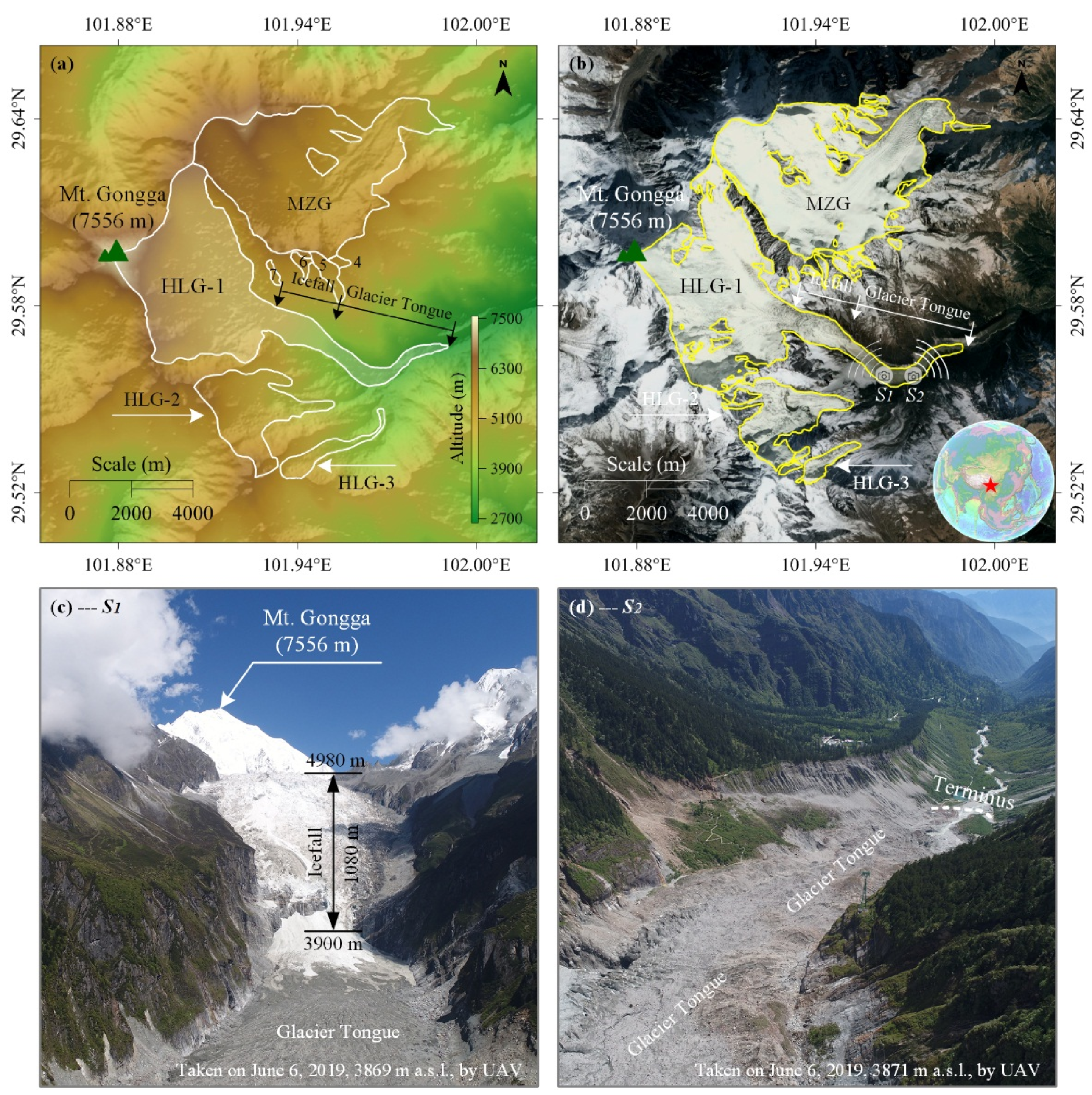
2.1. Study Area
2.2. Data Sets
3. Method
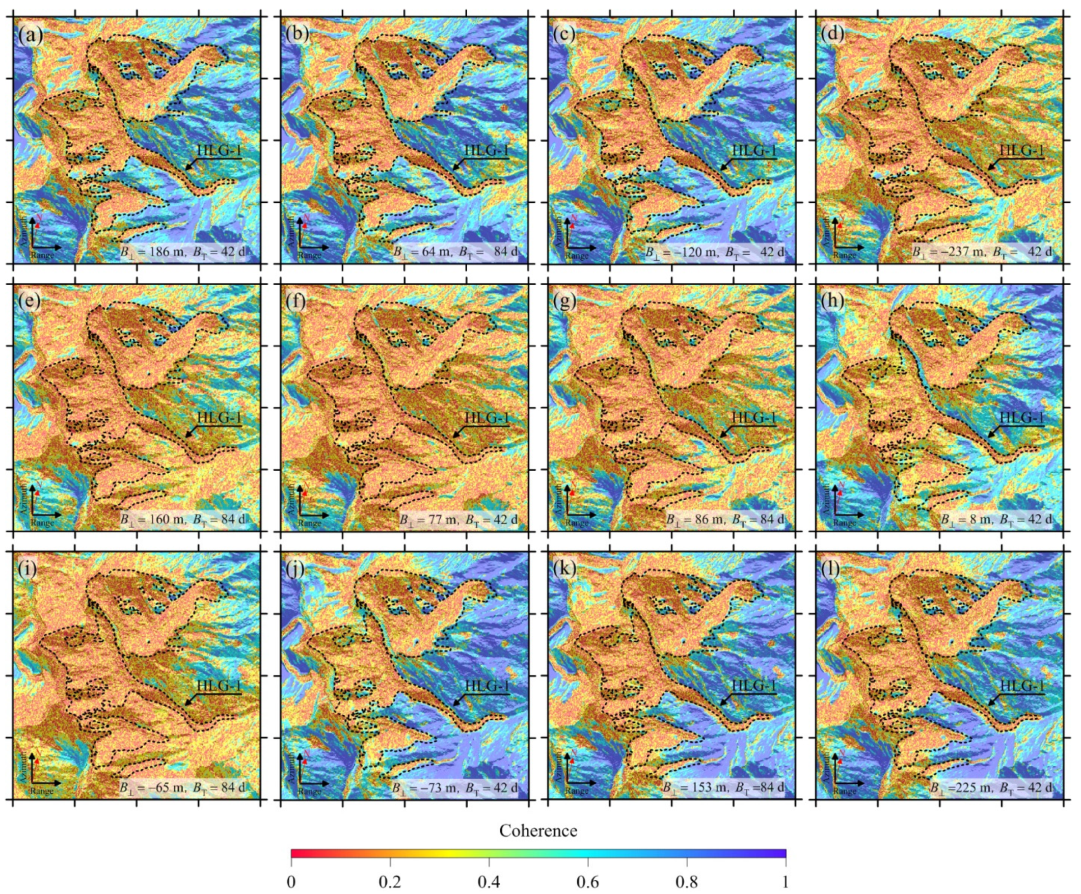
3.1. Coherence
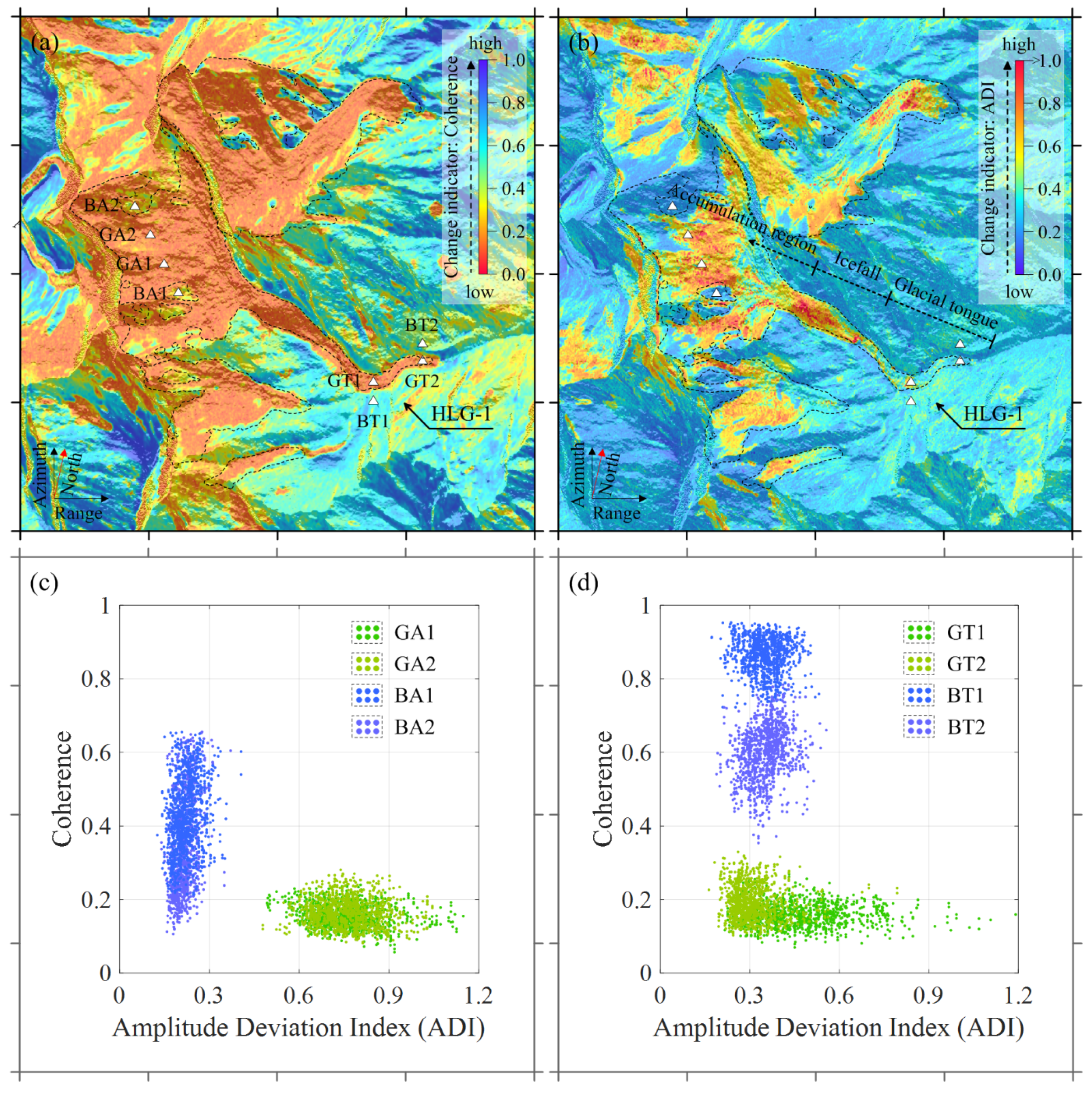
3.2. SAR Amplitude Dispersion Index
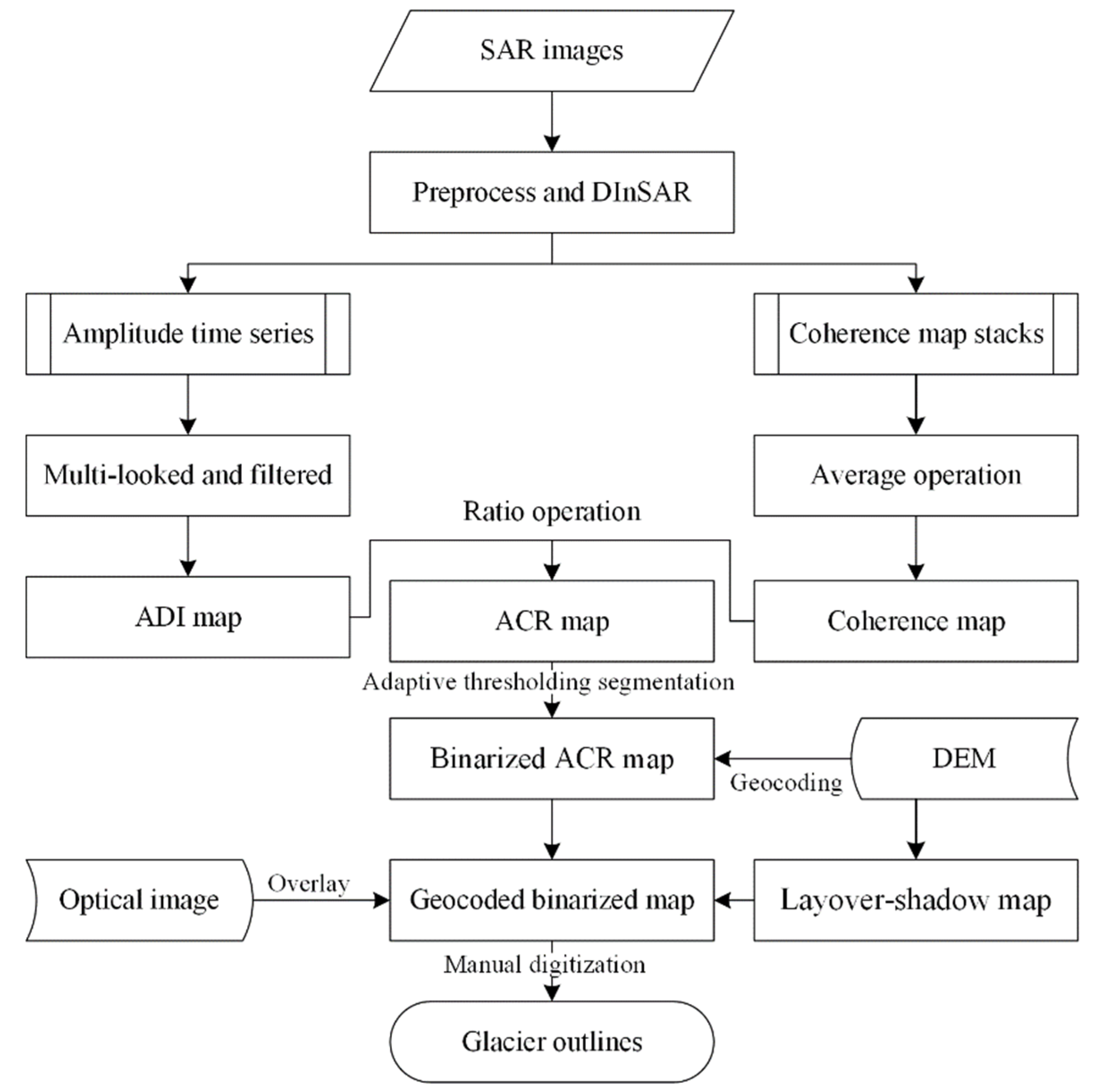
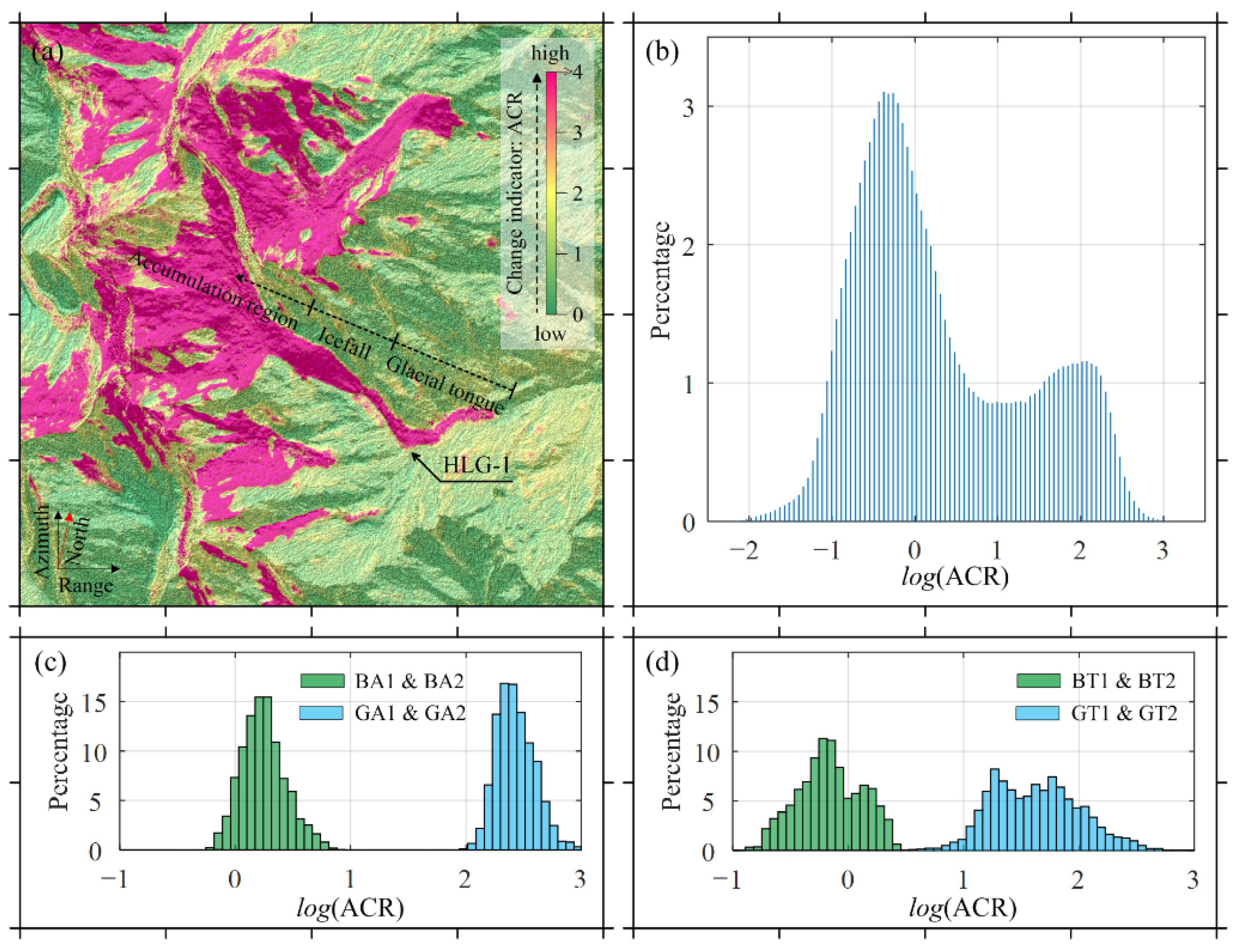
3.3. Generation of an ACR Map Combining ADI and Coherence
3.4. Delineating the Glacier Outlines by Combining the Classified ACR Map and an Optical Image
3.5. Accuracy Assessment
4. Results
4.1. Glacier Boundaries Delineated Based on the ACR Map
4.2. Validations of the Glacier Outlines from the ACR Map
5. Discussion
5.1. Comparisons with the Glacier Classifications from Satellite Optical Images
5.2. Comparisons of ACR with SAR Coherence for Glacier Classification
5.3. Limitations of Glacier Mapping Based on ACR
6. Conclusions
Author Contributions
Funding
Data Availability Statement
Acknowledgments
Conflicts of Interest
References
- Raup, B.; Kääb, A.; Kargel, J.S.; Bishop, M.P.; Hamilton, G.; Lee, E.; Paul, F.; Rau, F.; Soltesz, D.; Khalsa, S.J.; et al. Remote sensing and GIS technology in the Global Land Ice Measurements from Space (GLIMS) Project. Comput. Geosci. 2007, 33, 104–125. [Google Scholar] [CrossRef]
- Bishop, M.P.; Olsenholler, J.A.; Shroder, J.F.; Barry, R.G.; Raup, B.H.; Bush, A.B.G.; Copland, L.; Dwyer, J.; Fountain, A.G.; Haeberli, W.; et al. Global Land Ice Measurements from Space (GLIMS): Remote Sensing and GIS Investigations of the Earth’s Cryosphere. Geocarto Int. 2004, 19, 57–84. [Google Scholar] [CrossRef]
- Pfeffer, W.T.; Arendt, A.A.; Bliss, A.; Bolch, T.; Cogley, J.G.; Gardner, A.; Hagen, J.-O.; Hock, R.; Kaser, G.; Kienholz, C.; et al. The Randolph Glacier Inventory: A globally complete inventory of glaciers. J. Glaciol. 2014, 60, 537–552. [Google Scholar] [CrossRef] [Green Version]
- Guo, W.; Liu, S.; Xu, J.; Wu, L.; Shangguan, D.; Yao, X.; Wei, J.; Bao, W.; Yu, P.; Liu, Q.; et al. The second Chinese glacier inventory: Data, methods and results. J. Glaciol. 2015, 61, 357–372. [Google Scholar] [CrossRef] [Green Version]
- Nuimura, T.; Sakai, A.; Taniguchi, K.; Nagai, H.; Lamsal, D.; Tsutaki, S.; Kozawa, A.; Hoshina, Y.; Takenaka, S.; Omiya, S.; et al. The GAMDAM glacier inventory: A quality-controlled inventory of Asian glaciers. Cryosphere 2015, 9, 849–864. [Google Scholar] [CrossRef] [Green Version]
- Sakai, A. GAMDAM glacier inventory for High Mountain Asia. PANGAEA 2015. [Google Scholar] [CrossRef]
- Liu, Q.; Liu, S.Y.; Guo, W.Q.; Nie, Y.; Shangguan, D.H.; Xu, J.L.; Yao, X.J. Glacier Changes in the Lancang River Basin, China, between 1968–1975 and 2005–2010. Arctic Antarct. Alp. Res. 2015, 47, 335–344. [Google Scholar] [CrossRef] [Green Version]
- Wu, K.; Liu, S.; Jiang, Z.; Xu, J.; Wei, J.; Guo, W. Recent glacier mass balance and area changes in the Kangri Karpo Mountains from DEMs and glacier inventories. Cryosphere 2018, 12, 103–121. [Google Scholar] [CrossRef] [Green Version]
- Liu, Q.; Mayer, C.; Wang, X.; Nie, Y.; Wu, K.; Wei, J.; Liu, S. Interannual flow dynamics driven by frontal retreat of a lake-terminating glacier in the Chinese Central Himalaya. Earth Planet. Sci. Lett. 2020, 546, 116450. [Google Scholar] [CrossRef]
- Kargel, J.S.; Abrams, M.J.; Bishop, M.P.; Bush, A.; Hamilton, G.; Jiskoot, H.; Kääb, A.; Kieffer, H.H.; Lee, E.M.; Paul, F.; et al. Multispectral imaging contributions to global land ice measurements from space. Remote Sens. Environ. 2005, 99, 187–219. [Google Scholar] [CrossRef]
- Shukla, A.; Gupta, R.; Arora, M. Estimation of debris cover and its temporal variation using optical satellite sensor data: A case study in Chenab basin, Himalaya. J. Glaciol. 2009, 55, 444–452. [Google Scholar] [CrossRef] [Green Version]
- Bolch, T.; Menounos, B.; Wheate, R. Landsat-based inventory of glaciers in western Canada, 1985–2005. Remote Sens. Environ. 2010, 114, 127–137. [Google Scholar] [CrossRef]
- Paul, F.; Bolch, T.; Kääb, A.; Nagler, T.; Nuth, C.; Scharrer, K.; Shepherd, A.; Strozzi, T.; Ticconi, F.; Bhambri, R.; et al. The glaciers climate change initiative: Methods for creating glacier area, elevation change and velocity products. Remote Sens. Environ. 2015, 162, 408–426. [Google Scholar] [CrossRef] [Green Version]
- Kaushik, S.; Joshi, P.K.; Singh, T. Development of glacier mapping in Indian Himalaya: A review of approaches. Int. J. Remote Sens. 2019, 40, 6607–6634. [Google Scholar] [CrossRef]
- Racoviteanu, A.; Williams, M.W. Decision Tree and Texture Analysis for Mapping Debris-Covered Glaciers in the Kangchenjunga Area, Eastern Himalaya. Remote Sens. 2012, 4, 3078–3109. [Google Scholar] [CrossRef] [Green Version]
- Raup, B.; Khalsa, S.J.S. GLIMS Analysis Tutorial; National Snow: Boulder, CO, USA, 2010; Available online: http://www.glims.net/MapsAndDocs/assets/GLIMS_Analysis_Tutorial_a4.pdf (accessed on 22 February 2022).
- Goldstein, R.M.; Engelhardt, H.; Kamb, B.; Frolich, R.M. Satellite Radar Interferometry for Monitoring Ice Sheet Motion: Application to an Antarctic Ice Stream. Science 1993, 262, 1525–1530. [Google Scholar] [CrossRef]
- Strozzi, T.; Luckman, A.; Murray, T.; Wegmuller, U.; Werner, C. Glacier motion estimation using SAR offset-tracking procedures. IEEE Trans. Geosci. Remote Sens. 2002, 40, 2384–2391. [Google Scholar] [CrossRef] [Green Version]
- Winsvold, S.H.; Kääb, A.; Nuth, C.; Andreassen, L.M.; van Pelt, W.J.J.; Schellenberger, T. Using SAR satellite data time series for regional glacier mapping. Cryosphere 2018, 12, 867–890. [Google Scholar] [CrossRef] [Green Version]
- Friedl, P.; Weiser, F.; Fluhrer, A.; Braun, M.H. Remote sensing of glacier and ice sheet grounding lines: A review. Earth-Sci. Rev. 2020, 201, 102948. [Google Scholar] [CrossRef]
- Atwood, D.K.; Meyer, F.; Arendt, A. Using L-band SAR coherence to delineate glacier extent. Can. J. Remote Sens. 2010, 36, S186–S195. [Google Scholar] [CrossRef]
- Frey, H.; Paul, F.; Strozzi, T. Compilation of a glacier inventory for the western Himalayas from satellite data: Methods, challenges, and results. Remote Sens. Environ. 2012, 124, 832–843. [Google Scholar] [CrossRef] [Green Version]
- Robson, B.A.; Nuth, C.; Dahl, S.O.; Hölbling, D.; Strozzi, T.; Nielsen, P.R. Automated classification of debris-covered glaciers combining optical, SAR and topographic data in an object-based environment. Remote Sens. Environ. 2015, 170, 372–387. [Google Scholar] [CrossRef] [Green Version]
- Lippl, S.; Vijay, S.; Braun, M. Automatic delineation of debris-covered glaciers using InSAR coherence derived from X-, C- and L-band radar data: A case study of Yazgyl Glacier. J. Glaciol. 2018, 64, 811–821. [Google Scholar] [CrossRef] [Green Version]
- Shi, Y.; Liu, G.; Wang, X.; Liu, Q.; Zhang, R.; Jia, H. Assessing the Glacier Boundaries in the Qinghai-Tibetan Plateau of China by Multi-Temporal Coherence Estimation with Sentinel-1A InSAR. Remote Sens. 2019, 11, 392. [Google Scholar] [CrossRef] [Green Version]
- Zakhvatkina, N.; Smirnov, V.; Bychkova, I. Satellite SAR Data-based Sea Ice Classification: An Overview. Geosciences 2019, 9, 152. [Google Scholar] [CrossRef] [Green Version]
- Ferretti, A.; Prati, C.; Rocca, F. Permanent scatterers in SAR interferometry. IEEE Trans. Geosci. Remote Sens. 2001, 39, 8–20. [Google Scholar] [CrossRef]
- Wei, M.; Sandwell, D. Decorrelation of L-Band and C-Band Interferometry Over Vegetated Areas in California. IEEE Trans. Geosci. Remote Sens. 2010, 48, 2942–2952. [Google Scholar] [CrossRef]
- Liu, Q.; Liu, S.; Zhang, Y.; Wang, X.; Zhang, Y.; Guo, W.; Xu, J. Recent shrinkage and hydrological response of Hailuogou glacier, a monsoon temperate glacier on the east slope of Mount Gongga, China. J. Glaciol. 2010, 56, 215–224. [Google Scholar] [CrossRef] [Green Version]
- Hooper, A.; Segall, P.; Zebker, H. Persistent scatterer interferometric synthetic aperture radar for crustal deformation analysis, with application to Volcán Alcedo, Galápagos. J. Geophys. Res. Earth Solid Earth 2007, 112, 112. [Google Scholar] [CrossRef] [Green Version]
- Touzi, R.; Lopes, A.; Bruniquel, J.; Vachon, P.W. Coherence estimation for SAR imagery. IEEE Trans. Geosci. Remote Sens. 1999, 37, 135–149. [Google Scholar] [CrossRef] [Green Version]
- Werner, C.; Wegmüller, U.; Strozzi, T.; Wiesmann, A. Gamma SAR and interferometric processing software. In Proceedings of the Ers-Envisat Symposium, Gothenburg, Sweden, 16–20 October 2000. [Google Scholar]
- Ferretti, A.; Monti-Guarnieri, A.; Prati, C.; Rocca, F.; Massonnet, D. InSAR Principles: Guidelines for SAR Interferometry Processing and Interpretation; European Space Agency (ESA) Publications: Noordwijk, The Netherlands, 2007. [Google Scholar]
- Bradley, D.; Roth, G. Adaptive Thresholding using the Integral Image. J. Graph. Tools 2007, 12, 13–21. [Google Scholar] [CrossRef]
- Otsu, N. A threshold selection method from gray-level histograms. IEEE Trans. Syst. Man Cybern. 1979, 9, 62–66. [Google Scholar] [CrossRef] [Green Version]
- Basnett, S.; Kulkarni, A.V.; Bolch, T. The influence of debris cover and glacial lakes on the recession of glaciers in Sikkim Himalaya, India. J. Glaciol. 2013, 59, 1035–1046. [Google Scholar] [CrossRef] [Green Version]
- Alifu, H.; Tateishi, R.; Johnson, B. A new band ratio technique for mapping debris-covered glaciers using Landsat imagery and a digital elevation model. Int. J. Remote Sens. 2015, 36, 2063–2075. [Google Scholar] [CrossRef]
- Rignot, E.; Echelmeyer, K.; Krabill, W. Penetration depth of interferometric synthetic-aperture radar signals in snow and ice. Geophys. Res. Lett. 2001, 28, 3501–3504. [Google Scholar] [CrossRef] [Green Version]
- Brun, F.; Berthier, E.; Wagnon, P.; Kääb, A.; Treichler, D. A spatially resolved estimate of High Mountain Asia glacier mass balances from 2000 to 2016. Nat. Geosci. 2017, 10, 668–673. [Google Scholar] [CrossRef] [PubMed]
- Dehecq, A.; Gourmelen, N.; Gardner, A.S.; Brun, F.; Goldberg, D.; Nienow, P.W.; Berthier, E.; Vincent, C.; Wagnon, P.; Trouvé, E. Twenty-first century glacier slowdown driven by mass loss in High Mountain Asia. Nat. Geosci. 2019, 12, 22–27. [Google Scholar] [CrossRef]


| No. | Master | Slave | Perp-Baseline | Time Interval | Coherence Map |
|---|---|---|---|---|---|
| 1 | 20171201 | 20180112 | 186 m | 42 d | Figure 3a |
| 2 | 20171201 | 20180223 | 67 m | 84 d | Figure 3b |
| 3 | 20180112 | 20180223 | −120 m | 42 d | Figure 3c |
| 4 | 20180223 | 20180406 | −237 m | 42 d | Figure 3d |
| 5 | 20180223 | 20180518 | 160 m | 84 d | Figure 3e |
| 6 | 20180406 | 20180518 | 77 m | 42 d | Figure 3f |
| 7 | 20180406 | 20180629 | 86 m | 84 d | Figure 3g |
| 8 | 20180518 | 20180629 | 8 m | 42 d | Figure 3h |
| 9 | 20180518 | 20180810 | −65 m | 84 d | Figure 3i |
| 10 | 20180629 | 20180810 | −73 m | 42 d | Figure 3j |
| 11 | 20180629 | 20180921 | 153 m | 84 d | Figure 3k |
| 12 | 20180810 | 20180921 | 225 m | 42 d | Figure 3l |
| Sample No. | Category | Surface Features | ADI | Coherence | ACR |
|---|---|---|---|---|---|
| GA1 and GA2 | Glacier | Pure ice | high | low | high |
| GT1 and GT2 | Glacier | Moraine | both | low | high |
| BA1 and BA2 | Non-glacier | Bedrock | low | high | low |
| BT1 and BT2 | Non-glacier | Bare soil and vegetation | low | high | low |
| - | Area (km2) | Type | ||
|---|---|---|---|---|
| ACR | SCGI | GGI | - | |
| HLG-1 | 21.47 | 24.59 | 24.60 | V |
| HLG-2 | 5.26 | 7.32 | 5.89 | V |
| HLG-3 | 0.82 | 1.60 * | 0.99 | H |
| HLG-4 | 0.16 | NR | H | |
| HLG-5 | 0.13 | 0.18 | 0.38 | H |
| HLG-6 | 0.15 | 0.79 | 0.42 | H |
| HLG-7 | 0.07 | 0.30 | 0.21 | H |
| HLG-8 | 0.06 | NR | 0.12 | H |
| HLG-9 | 0.22 | 0.20 | 0.12 | H |
| MZG-1 | 23.70 | 25.88 | 25.80 | V |
| MZG-2 | 0.14 | NR | 0.24 | H |
| MZG-3 | 0.03 | NR | 0.29 * | H |
| MZG-4 | 0.07 | NR | H | |
| Total | 52.28 | 60.85 | 58.75 | - |
| - | Ground Truth | ACR | GGI | SCGI |
|---|---|---|---|---|
| Area (km2) | 5.66 | 5.41 | 6.21 | 7.31 |
| Difference (km2) | - | −0.25 | 0.55 | 1.65 |
| Difference rate | - | 4.4% | 9.7% | 29.1% |
| Misclassification | - | 2.6% | 3.9% | 13.8% |
| Deficiency | 4.2% | 2.7% | 4.5% |
Publisher’s Note: MDPI stays neutral with regard to jurisdictional claims in published maps and institutional affiliations. |
© 2022 by the authors. Licensee MDPI, Basel, Switzerland. This article is an open access article distributed under the terms and conditions of the Creative Commons Attribution (CC BY) license (https://creativecommons.org/licenses/by/4.0/).
Share and Cite
Zhang, B.; Liu, G.; Wang, X.; Fu, Y.; Liu, Q.; Yu, B.; Zhang, R.; Li, Z. Semi-Automated Mapping of Complex-Terrain Mountain Glaciers by Integrating L-Band SAR Amplitude and Interferometric Coherence. Remote Sens. 2022, 14, 1993. https://doi.org/10.3390/rs14091993
Zhang B, Liu G, Wang X, Fu Y, Liu Q, Yu B, Zhang R, Li Z. Semi-Automated Mapping of Complex-Terrain Mountain Glaciers by Integrating L-Band SAR Amplitude and Interferometric Coherence. Remote Sensing. 2022; 14(9):1993. https://doi.org/10.3390/rs14091993
Chicago/Turabian StyleZhang, Bo, Guoxiang Liu, Xiaowen Wang, Yin Fu, Qiao Liu, Bing Yu, Rui Zhang, and Zhilin Li. 2022. "Semi-Automated Mapping of Complex-Terrain Mountain Glaciers by Integrating L-Band SAR Amplitude and Interferometric Coherence" Remote Sensing 14, no. 9: 1993. https://doi.org/10.3390/rs14091993
APA StyleZhang, B., Liu, G., Wang, X., Fu, Y., Liu, Q., Yu, B., Zhang, R., & Li, Z. (2022). Semi-Automated Mapping of Complex-Terrain Mountain Glaciers by Integrating L-Band SAR Amplitude and Interferometric Coherence. Remote Sensing, 14(9), 1993. https://doi.org/10.3390/rs14091993