Article

Impact of BRDF Spatiotemporal Smoothing on Land Surface Albedo Estimation

1
College of Surveying and Mapping and Geographic Science, Liaoning Technical University, Fuxin 123000, China
2
Xinjiang Institute of Ecology and Geography, Chinese Academy of Sciences, Urumqi 830011, China
3
University of Chinese Academy of Sciences, Beijing 100049, China
4
Research Center for Ecology and Environment of Central Asia, Chinese Academy of Sciences, Urumqi 830011, China
5
State Key Laboratory of Remote Sensing Science, Faculty of Geographical Science, Beijing Normal University, Beijing 100875, China
6
School of Aeronautics and Astronautics, Sun Yat-sen University, Guangzhou 510006, China
*
Author to whom correspondence should be addressed.
These authors contributed equally to this work.
Remote Sens. 2022, 14(9), 2001; https://doi.org/10.3390/rs14092001
Submission received: 28 March 2022 / Revised: 18 April 2022 / Accepted: 19 April 2022 / Published: 21 April 2022
(This article belongs to the Special Issue Remote Sensing for Surface Biophysical Parameter Retrieval)

Abstract

:
Surface albedo, as a key parameter determining the partition of solar radiation at the Earth’s surface, has been developed into a satellite-based product from various Earth observation systems to serve numerous global or regional applications. Studies point out that apparent uncertainty can be introduced into albedo retrieval without consideration of surface anisotropy, which is a challenge to albedo estimation especially from observations with fewer angular samplings. Researchers have begun to introduce smoothed anisotropy prior knowledge into albedo estimation to improve the inversion efficiency, or for the scenario of observations with signal or poor angular sampling. Thus, it is necessary to further understand the potential influence of smoothed anisotropy features adopted in albedo estimation. We investigated the albedo variation induced by BRDF smoothing at both temporal and spatial scales over six typical landscapes in North America using MODIS standard anisotropy products with high quality BRDF inversed from multi-angle observations in 500 m and 5.6 km spatial resolutions. Components of selected typical landscapes were assessed with the confidence of the MCD12 land cover product and 30 m CDL (cropland data layer) classification maps followed by an evaluation of spatial heterogeneity in 30 m scale through the semi-variogram model. High quality BRDF of MODIS standard anisotropy products were smoothed in multi-temporal scales of 8 days, 16 days, and 32 days, and in multi-spatial scales from 500 m to 5.6 km. The induced relative and absolute albedo differences were estimated using the RossThick-LiSparseR model and BRDFs smoothed before and after spatiotemporal smoothing. Our results show that albedo estimated using BRDFs smoothed temporally from daily to monthly over each scenario exhibits relative differences of 11.3%, 12.5%, and 27.2% and detectable absolute differences of 0.025, 0.012, and 0.013, respectively, in MODIS near-infrared (0.7–5.0 µm), short-wave (0.3–5.0 µm), and visible (0.3–0.7 µm) broad bands. When BRDFs of investigated landscapes are smoothed from 500 m to 5.6 km, variations of estimated albedo can achieve up to 36.5%, 37.1%, and 94.7% on relative difference and absolute difference of 0.037, 0.024, and 0.018, respectively, in near-infrared (0.7–5.0 µm), short wave (0.3–5.0 µm), and visible (0.3–0.7 µm) broad bands. In addition, albedo differences caused by temporal smoothing show apparent seasonal characteristic that the differences are significantly higher in spring and summer than those in autumn and winter, while albedo differences induced by spatial smoothing exhibit a noticeable relationship with sill values of a fitted semi-variogram marked by a correlation coefficient of 0.8876. Both relative and absolute albedo differences induced by BRDF smoothing are demonstrated to be captured, thus, it is necessary to avoid the smoothing process in quantitative remote sensing communities, especially when immediate anisotropy retrievals are available at the required spatiotemporal scale.

Graphical Abstract

1. Introduction

Land surface albedo, defined as the ratio of upwelling to downwelling solar radiation at the land surface over the whole solar spectrum, is an important parameter determining the partition of solar energy between Earth’s surface and atmosphere [1,2]. Surface albedo quantifies the solar energy intercepted by components within various ecosystems to trigger more energy cycles, such as the phase transition of water via latent heat and heat transfer through conduction, convection, or radiation within components of biogeophysical and biogeochemical processes [2,3,4,5]. Land surface albedo is a major parameter of land surface models and directly affects the heat and water-vapor exchange between ground and atmosphere [6]. The budget of energy between ground and atmosphere is influenced by surface albedo, thus it affects the atmospheric movement and medium/long-term weather forecast [7]. Albedo changes due to land use/cover change (LUCC) such as deforestation have a profound impact on surface net radiation flux, which should not be ignored in the study of land surface temperature and monsoon [8,9,10]. Therefore, land surface albedo is valuable for studies of land surface models, circulation models, LUCC and the global climate.
The accuracy requirements of albedo keep increasing with the need from various user communities or with increasing understanding of processes of earth systems. An albedo accuracy of 0.02–0.05 is required by the community of global climate change [11,12] but increases to 0.02 for regional investigations [13]. Further, a revised land surface model based on albedo with higher accuracy could modify the predicted net radiation and sensible heat exchange by 5–30% [14]. A 10% error in albedo for agricultural landscape may induce a relative uncertainty in net radiation of 5% [15]. In evapotranspiration investigation, an uncertainty of 10% in albedo can introduce a potential error of 20 W/m2 in net radiation [16]. Therefore, accurate surface albedo is important to achieve relevant energy estimation for numerous molders or applications in ecosystems, the carbon cycle, and climate communities [14,17].
Satellite remote sensing is the only way to routinely produce regional or global albedo. In the early stage, observations with a single angle were the dominant scheme provided by satellite-based sensors. Later, multi-angle sensors represented by POLDER and MISR were launched with the ability to simultaneously provide multi-angle observations [18,19,20]. In addition, multi-angle observations can be achieved in wide-swath satellite images with a trade-off between angles and time [21,22,23]. Compared with previous signal-angle estimation, modern albedo algorithms rely on multiple-angle observations to first build a BRDF (bi-directional reflectance distribution function), then integrate over incident and view hemispheres to calculate albedo. Studies have pointed out that the relative errors can reach up to 45% in inferring hemispherical reflectance from nadir reflectance without consideration of angle effects [24,25]. Thus, multi-angle observations are essential to inverse the BRDF model and guarantee the estimation of albedo accuracy.
BRDF was defined by Nicodemus in 1977 [26] and has been accepted widely as an intrinsic feature of land cover. Numerous studies have demonstrated that ground, airborne, or spaceborne observations exhibit obvious angle-effect phenomena [27,28,29]. BRDF theoretically describes the variation of directional reflectance in terms of incident-view geometry within both hemispheres [22,30,31,32]. Multi-angle observations have been collected from ground measurements and several satellite sensors, such as POLDER [33], MISR, and MSG, and MODIS and AVHRR have achieved angle sampling from overlapped swaths within a given period. The standard BRDF products retrieved from multi-angle satellite observations include the MODIS nominal daily anisotropy dataset at spatial scales from 500 m to 5.6 km [34], POLDER at 6 km by 7 km spatial scale, and some other sporadic anisotropic products.
Anisotropy information at fine resolution is needed in the retrieval of surface albedo in the tens of meters spatial resolution. Compared with observations at kilometers, satellites providing observations at fine resolution are required to collect surface details in global or regional areas, such as the Sentinel series of Europe, the Landsat series of the United States, and the HuanJing and GF series of China. However, these observation systems can’t provide instantaneous multi-angle observations, nor trade-off angle with time through swath overlapping. Thus, researchers have begun to introduce BRDF priori knowledge into surface albedo retrieval, especially at high spatial resolution due to the lack of multi-angle observations. Shuai et al., 2011 and 2014, proposed the MODIS-Concurrent algorithm, which combined MODIS 500 m BRDF with corresponding Landsat surface reflectance to estimate surface albedo at 30 m resolution [35], followed by an extension to the pre-MODIS era, back to the 1980s, through an anisotropic LUT (look-up table) established from high-quality 500 m MCD43A-BRDF data [36]. Franch used smoothed 5.6 km MODIS BRDF with a further adjustment by NDVI in their VJB method, then decomposed it to estimate 30 m Landsat surface albedo [37,38]; Jiao established a BRDF archetype database by using a clustering algorithm and parameter smoothing of BRDF based on anisotropic flat index (AFX) [39,40]. Zhang Hu estimated surface albedo based on the archetype database classified by AFX [41]. However, there is a lack of understanding of the difference within estimated albedo induced by the anisotropy information smoothed at spatiotemporal scales. This work will focus on this issue to investigate the effects of smoothed BRDF on albedo magnitude through case studies using MODIS operational BRDF products.

2. Study Sites and Data

2.1. Study Sites

Six study sites in the MODIS golden tile H09V05 in the Southwestern United States were selected to cover rich types of land surface as the study region (92.38°W to 117.49°W, 30°N to 40°N). Details of the six selected sites are shown in Table 1, which includes the IGBP classification type, location, and climate zone.

2.2. MODIS Products

We selected MODIS BRDF/Albedo products in three broad bands which are near-infrared (NIR, 0.7–5.0 µm), short wave (SW, 0.3–5.0 µm), and visible (VIS, 0.3–0.7 µm) at 500 m and 5.6 km resolutions, and land cover products (Table 2), which we downloaded from the NASA official open data pool (https://ladsweb.modaps.eosdis.nasa.gov/search/ (accessed on 30 January 2021)). The operational MODIS BRDF/Albedo algorithm assumes that the land surface does not change significantly during the period of data accumulation (16 days), but with a further enhancement on the observations close to the retrieval day in the nominal daily inversion. The kernel-driven linear model expressed as RossThick-LiSparseR is adopted to determine the kernel parameters f i s o   f g e o   f v o l respectively for isotropic kernel, K i s o ; volumetric scattering kernel, K v o l ; and geometric kernel, K g e o , to estimate the gridded 500 m and 5600 m BRDF/Albedo at that shown in Equation (1), where λ is the spectral band [22,34].
R e f l e c t a n c e = f i s o λ k i s o + f g e o λ k g e o + f v o l λ k v o l
MODIS land cover products MCD12C1 and MCD12Q1 provide global land cover maps at 5600 m and 500 m, at annual time steps. The MCD12Q1 product is produced using supervised classification of MODIS Nadir BRDF-adjusted reflectance and MCD12C1 is aggregated and reprojected from 500 m MCD12Q1 products [42,43]. MODIS land cover type products had an overall accuracy of 75% by cross-validation accuracy assessment [43] and the majority class confidence can assist to assess majority land cover type in MCD12C1 pixels. IGBP contains 17 types of land cover, and its original data source (AVHRR) and goal of modeling biophysical parameters of land surface is similar to MODIS [42,43,44,45]. Thus, we selected IGBP in MCD12C1 and MCD12Q1 to provide the classification of land cover.

2.3. CDL Database

CDL (cropland data layer) annually produced by USDA-NASS (United States Department of Agriculture-National Agricultural Statistics Service) is a geospatial crop-specific open 30 m land cover thematic dataset and serving numerous user communities. The 2019 CDL is generated from Landsat-8 OLI/TIRS, DEIMOS-1, UK2, LISS-3 of ResourceSat-2, SENTINEL-2A/B and downloaded from https://nassgeodata.gmu.edu/CropScape/ (accessed on 16 February 2021). The crop-specific classification map with a spatial resolution of 30 m, covering the continental United States, is produced by satellite imagery. The quality of CDL is high, with the total crop mapping accuracies ranging from 85% to 95% for the major crop categories [46]. The accuracy of CDL in non-agricultural land cover classes ranges from 82–89% depending upon the USGS, National Land Cover Database (NLCD) [47]. We selected CDL to assess the land cover types in MODIS pixels in detail.

2.4. Landsat-8 Dataset

To evaluate the spatial heterogeneity of land surface in pixels at coarse spatial scale, the corresponding land surface albedo at higher resolution is needed as the basic data. The Landsat-8 satellite is in a sun-synchronous, near-polar, 705 km circular orbit and can produce scenes within 185 km × 180 km. Compared with MODIS, Landsat-8 OLI (operational land imager) can provide reflectance product of land cover at a spatial resolution of 30 m and can be used to reconstruct the surface albedo at 30 m. Landsat-8 has a repeat cycle of 16 days, which can provide sequential repeated images 22 or 23 times for a fixed location per year [48]. Landsat-8 OLI provides spectral reflectance information of land cover in 9 bands from visible to shortwave infrared. We selected landsat-8 OLI surface reflectance products after radiometric and geometric correction under cloud-free condition in 2019 as the basic data and the datasets for six study sites were downloaded from https://earthexplorer.usgs.gov/ (accessed on 15 August 2021).

2.5. Data Preprocessing

A series of preprocessing steps were performed, including the selection and assessment of study areas, re-projection between different products, and screening of high quality BRDF/Albedo. MODIS land cover type products (MCD12C1 and MCD12Q1) were used to determine specific study pixels (500 m). MCD12C1 IGBP layer in 5600 m scale was used to choose study sites with high confidence, followed by reprojection to the 500 m IGBP layer of MCD12Q1 (Figure 1). From Figure 1, we can see that a representative site (500 m) is selected from homogeneous underlayer with the pixels of the same land cover type around.
To further analyze the internal land cover types in MODIS pixels (5600 m and 500 m), CDL pixels were counted to show the proportions of land cover categories within MODIS pixels (5600 m and 500 m) (Figure 2). It can be seen from Figure 2a–l that, compared with pixels at 5600 m, the proportions of the main categories at 500 m are significantly higher, which indicates that pixels at 500 m are more homogeneous, which is consistent with conventional cognition (the larger the range, the more complex the land cover). We selected the representative MODIS pixels (500 m) with homogeneous underlayer for the study of temporal smoothing, together with their corresponding MODIS pixels at 5600 m for the study of spatial smoothing.
To focus on the investigation of targets located on the land surface, observations contaminated by snow and cloud were removed from the temporal MODIS data series using the snow and cloud flag. Further, high-quality MODIS BRDF and albedo data labeled by related pixel-based QA (0, 1, 2) were screened out from collected datasets. This could not only ensure the acquisition of sufficient DOYs (days of the year) in 2019 with high-quality, but also eliminate the impact of data with low quality to a great extent.
In addition, Re-projection is required between different datasets. MODIS products with spatial resolution of 5600 m adopt longitude and latitude projection, while MODIS products with spatial resolution of 500 m use Sinusoidal projection (Table 2) [49,50,51]. The CDL uses Albers projection, while landsat-8 is UTM (universal transverse Mercator) projection [46,48]. When conversion was required between different types of datasets, re-projection processing was performed: (1) in order to investigate the classification within MODIS pixels (5600 m), MCD12C1 pixels were re-projected to MCD12Q1 products; (2) in order to investigate the type complexity of MODIS pixels in detail, MCD12C1 and MCD12Q1 pixels were re-projected to CDL; (3) to assess the surface heterogeneity, MCD12C1 pixels were re-projected to landsat-8 OLI images.

3. Method

3.1. Strategy of Spatiotemporal Smoothing

To obtain BRDF in multi-temporal scales, BRDF parameters of land surface are smoothed in different temporal scales (8 days–16 days–1 month), see Figure 3a. As BRDF can be represented by a kernel-driven linear model (Equation (1)), smoothed BRDF can also be represented by these smoothed model parameters (Equation (2)), where f k is the parameter of the isotropic, volumetric, geometric-optical kernel, scale is 8 days, 16 days, or a month, respectively, and N is the number of scale periods. To maintain the consistency of the temporal range, the number of days in the monthly scale is set to 32 days. It should be noted that the MCD43A1 is named ‘daily’ though it is a nominal daily period and is the weighted synthesis of surface reflectance under clear sky over a 16-day period.
f s m o o t h e d k = i = 1 S c a l e f k i N
For BRDF smoothing in multi-spatial scales (Figure 3b), as MODIS provides two BRDF products (MCD43A and MCD43C) at different resolutions (500 m and 5600 m), we directly extracted BRDF parameters from these datasets to represent BRDF before and after spatial smoothing. Here, we obtained BRDF parameters before and after smoothing in multi-spatiotemporal scales and the reflectance under any incident-view geometry could be inversed based on a set of fixed BRDF parameters. In this paper, the research version of the operating AMBLARS algorithm [22,30,52], provided by Boston University, was used to retrieve reflectance under given incident-view geometries based on RossThick-LiSparseR model.
According to the integral mode, MODIS-albedo can be defined as: black sky albedo (BSA), which is the integration of BRDF in the view hemisphere with direct incident light (Equation (3)); white sky albedo (WSA), which is the integration of BRDF in both incident and view hemispheres with isotropic incident light (Equation (4)). In Equations (3) and (4), θ i   and   i are zenith and azimuth angles of incident solar direction; θ r   and   r are zenith and azimuth angles of view direction, and f r θ i , i ; θ r , r is the BRDF function. Both the BSA and WSA are based on a set of fixed kernel coefficients to integrate in hemispherical or bi-hemispherical space. Theoretically, albedo obtained from BRDF parameters at the coarse scale after spatial and temporal smoothing is consistent with the smoothed value of albedo before smoothing (Equation (5), and θ   and   are the zenith and azimuth angle in hemispherical or bi-hemispherical space).
B S A = 0 2 π 0 π / 2 f r θ i , i ; θ r , r sin θ r cos θ r d θ r d r
W S A = 1 π 0 2 π 0 π / 2 ( B S A ) sin θ i cos θ i d θ i d i
i = 1 N f i s o i N k i s o + i = 1 N f g e o i N k g e o + i = 1 N f v o l i N k v o l sin θ cos θ d θ d = i = 1 N ( f i s o i k i s o + f g e o i k g e o + f v o l i k v o l sin θ cos θ d θ d ) / N
As MODIS provides two albedo products (MCD43A3 and MCD43C3) at different resolutions (500 m and 5600 m), we extracted albedo from MCD43A3 and smoothed daily albedo in multi-temporal scales to represent the integration of the corresponding smoothed BRDF, meanwhile we directly extracted albedo from MCD43C3 to represent the integration of the corresponding smoothed BRDF in multi-spatial scales. The workflow of this paper is shown in Figure 4.

3.2. Differences of BRDF

In the view hemisphere, the principal plane, which is determined by the directions of incident illumination and outgoing reflectance that intersect at the identical target, implies typical anisotropy features, such as variations in reflectance in magnitude and shapes of BRDF (Figure 5a). In this paper, the difference in BRDF is investigated by comparing the magnitude and shape between BRDF principal planes. The average reflectance with an interval of 1° from −70° (backward) to 70° (forward) was used to describe magnitude of principal plane (Equation (6)).
To describe the change in BRDF shape, we took ±70°, ±45°, LSN (local solar noon), zenith direction as characteristic directions and calculated differences in reflectance compared to smoothed BRDF at characteristic directions (Figure 5b and Equation (7), where N is the number of principal planes to be compared and j is ±70°, ±45°, LSN, 0°, respectively, and Fixed-Reflectance stands for the smoothed principal planes). Furthermore, the SD (standard deviation) of differences of reflectance at characteristic directions is adopted to measure the variation in the shape of BRDF (Equation (8)). If the distribution of differences in reflectance in the six characteristic directions is relatively concentrated, it indicates that the differences in reflectance in the six characteristic directions is relatively uniform and the difference between BRDF shapes is small, meanwhile the SD is smaller in this situation. On the contrary, a larger SD means that the difference between the shapes of BRDF is greater.
Magnitude BRDF = i = 70 70 R e f l e c t a n c e i 141
D i f f e r e n c e j = i = 1 N R e f l e c t a n c e i j F i x e d R e f l e c t a n c e j N
Standard   Deviation BRDF = j = 1 6 D i f f e r e n c e j D i f f e r e n c e ¯ 2 6 1

3.3. Differences of Albedo

Albedo is a hemispherical integration of BRDF, the magnitude and shape of BRDF have potential impacts on albedo. MODIS-albedo products are available in two types: WSA and BSA. Considering that WSA is highly correlated with BSA [53,54], we selected WSA as the albedo before and after BRDF smoothing to serve for the difference comparison.
To explore differences in albedo caused by temporal smoothing of BRDF, as shown in Figure 3a, first, smoothed monthly values of albedo for 12 months were calculated; then, the smoothed albedo values at 16-day and 8-day scales within one month were calculated; Lastly the daily albedo values were compared with the corresponding smoothed albedo values in three broad bands: near-infrared (NIR), short wave (SW), and visible (VIS). We selected the relative and absolute differences in albedo to describe the relationship between them (Equations (9) and (10), where scales are 8 days, 16 days, and 32 days). Through the absolute and relative differences in albedo, we can quantitatively analyze the difference in daily albedo from smoothed albedo in a specific temporal scale.
When discussing the influence of BRDF spatial smoothing on the retrieval of albedo, we extracted albedo at 500 m and 5600 m from MCD43A3 and MCD43C3 products, then calculated the relative and absolute differences between them. Lastly, we counted the daily differences to explore the magnitudes of the differences (Figure 3b). Albedo difference due to BRDF spatial smoothing can be calculated by Equations (11) and (12), where N is the number of MODIS-pixels at 500 m within one MODIS pixel at 5600 m.
R e l a t i v e   d i f f e r e n c e temporal = i = 1 s c a l e WSA i WSA s m o o t h e d WSA s m o o t h e d scale
A b s o l u t e   d i f f e r e n c e temporal = i = 1 s c a l e WSA i WSA s m o o t h e d scale
R e l a t i v e   d i f f e r e n c e spatial = i = 1 N WSA 500 m i WSA 5600 m WSA 5600 m N
A b s o l u t e   d i f f e r e n c e spatial = i = 1 N WSA 500 m i WSA 5600 m N

3.4. Semi-Variogram

The spatial heterogeneity is related to the distribution and complexity of land cover, and the different land cover is related to albedo differences. A semi-variogram model is an effective way to describe heterogeneity of land cover, and its model parameters have a certain corresponding relationship with the landscape pattern. Some studies have used a semi-variogram function to evaluate the homogeneity of land cover and applied it to assess the spatial representativeness of ground tower measurement points [55,56,57,58]. As the landscape pattern may affect the distribution of spatial albedo, we analyzed the correlation between the land surface heterogeneity described by semi-variogram parameters and the differences in albedo due to BRDF spatial smoothing.
In order to evaluate the spatial heterogeneity within MODIS pixels, the surface albedo at 30 m needed to be reconstructed based on landsat-8 images under cloud-free weather in 2019. Among the 22 or 23 images over the whole year, we selected images from leaf-on or leaf-off stages under cloud-free weather to compare the seasonality of the surface. To completely cover MODIS pixels, we made a semi-variogram analysis of land cover within 6 km (slightly greater than 5600 m), centered on the selected study sites. The specific steps were as follows:
(1)
Pixels corresponding to the study sites were extracted from Landsat-8 OLI surface reflectance products in band 2 to band 7;
(2)
Narrowband-to-broadband parameters were used to produce albedo in three broad bands (near-infrared, short wave, and visible) from Landsat-8 pixels. As the imaging bands of Landsat OLI are different from the three broadbands in MODIS products, narrowband-to-broadband conversion was required (Equations (13)–(15)), where α is the albedo in the corresponding band [59,60];
(3)
Equation (16) was used to calculate half the average-squared-difference between pixels with three broadband albedos. The parameters of the semi-variogram model, such as range and sill, were fitted by sequential half the average-squared-difference (Equation (17)). In Equations (16)–(17), h is the lag distance, N(h) is the number of pixel pairs corresponding to h, Z x is the albedo at location x, C 0 is the nugget, C is the sill, and a is the range.
Range (a) describes the correlation distance of point pairs in study sites. There is a certain correlation between point pairs within range distance, and there is no correlated attribute between point pairs beyond this distance. Range is of great significance to judge spatial representativeness between different scales. Sill (C) describes the intensity of albedo change, and a smaller sill represents a more homogeneous land cover. In this paper, the area around the samples is fixed (6 km, covering 5600 m pixel), and sill (C) is used to analyze the heterogeneity of land cover.
α V I S = 0.5621 α 2 + 0.1479 α 3 + 0.2512 α 4 0.0015
α N I R = 0.5911 α 5 + 0.3155 α 6 + 0.0731 α 7 + 0.0019
α S W = 0.2453 α 2 + 0.0508 α 3 + 0.1804 α 4 + 0.3081 α 5 + 0.1332 α 6 + 0.0521 α 7 + 0.0011
γ E h = i = 1 N h Z x i Z x i + h 2 N h 0.5
γ E h = C 0 + C 1.5 h a 0.5 h a 3                 0 h a C 0 + C                                                                         h > a

4. Results and Analysis

4.1. Vegetation Index

EVIs shown in Figure 6a were calculated from the zenith reflectance provided by MCD43A4. Then, the seasonal distribution of EVI could be counted according to spring (March to May), summer (June to August), autumn (September to November) and winter (December, January and February) (Figure 6b). EVI (enhanced vegetation index) can reflect the growth and coverage of land cover and has a significant advantage in vegetation saturation, atmospheric impact, and soil background compared with other vegetation indexes [61,62,63]. It can be seen from Figure 6a,b that, generally, the EVIs of land cover in spring and summer are higher than in autumn and winter, which indicates that vegetation has a stronger growth state and higher coverage in spring and summer, which are more suitable for growth. But for EBF, the EVI in spring is slightly lower than that in autumn. This may be attributed to the change in EVI over the whole year being relatively mild for EBF growing in four seasons, and that the EVI in winter is high, resulting in a high EVI in autumn as the transition between summer and winter. For ENF, we only extracted data without snow from June to November, while the EVI in summer is higher than autumn. For DBF, Savannas, Grassland, and Cropland, EVI shows the obvious seasonal characteristic that EVIs in spring and summer are higher.

4.2. Spatial Heterogeneity

Figure 7a,b shows that the sill (C) values corresponding to the long horizontal lines of the spherical model (one of the fitting methods for the semi-variogram) on day 205 of 2019 (DOY 205) in three broad bands (1226 × 10−6, NIR; 454 × 10−6, SW; 128 × 10−6 VIS) are significantly lower than those on day 365 of 2019 (2196 × 10−6, NIR; 971 × 10−6, SW; 320 × 10−6, VIS). This is consistent with Figure 7c,d, which shows that the spatial heterogeneity of Savanna on day 205 of 2019 is lower than that on day 365 of 2019 (DOY 365). The reason can be explained as smaller sill (C) corresponding to lower spatial heterogeneity of land cover, and sill (C) being an effective parameter to describe spatial heterogeneity.
Table 3 shows the parameters of the semi-variogram for each study site in leaf-on and leaf-off seasons, corresponding to the growing and senescence seasons. For DBF, Savanna and Grassland samples with four distinct seasons, sill (C) values in the senescence season are significantly higher than those in the growing season. In the NIR and SW bands, Cropland shows similar characteristic to other samples, but the heterogeneity of the VIS band in winter (DOY352, 842 × 10−6) is lower than that in summer (DOY192, 1128 × 10−6) due to crop rotation and other factors. Meanwhile, the spatial heterogeneity of samples growing in four seasons is more complex. The sill (C) value of EBF on DOY319 within the senescence season is smaller than on DOY207, which indicates that spatial homogeneity is lower. However, heterogeneity of ENF in late autumn (DOY277) is higher than that in early autumn (DOY247). This shows that variation in land surface heterogeneity with temporal series is very complex. Therefore, we took the DOYs with Landsat8 OLI images to explore the relationship between the albedo difference due to BRDF spatial smoothing and the spatial heterogeneity.

4.3. Variation of BRDF Smoothing

4.3.1. Temporal Smoothing of BRDF

Figure 8 shows the principal planes after BRDF smoothing in one month compared with daily BRDF over selected study sites. We took June of 2019, in which the EVI level is high, as an example to show the variation in BRDF smoothing. It can be seen from Figure 8 that, compared with daily BRDF, the magnitudes and shapes of smoothed BRDF have changed after temporal smoothing. In addition, smoothed BRDF is almost in the middle location of daily principal plane curves and the ability to capture features of BRDF is reduced. To quantify the changes in BRDF, the difference in magnitude (Equation (6)) and standard deviation of multi-characteristic directions (Equations (7) and (8)) within principal planes were to be counted (Figure 9).
Figure 9a,b shows that the magnitude difference is largest in the NIR band and lowest in the VIS band for each selected study site, for example, the magnitude differences in the NIR, SW, and VIS bands are 0.63%, 0.27%, and 0.09%, respectively, for ENF in 2019/06. The standard deviation of each study site shows a similar characteristic in that the average SDs in the NIR, SW, and VIS bands are 0.32, 0.20, and 0.14, respectively. This indicates that the dispersion and shape change of BRDF are also gradually decreasing from the NIR and SW to the VIS band in 2019/06, which is consistent with the information shown in Figure 8.
Figure 9c,d shows the statistics of average magnitude difference and standard deviation in principal planes in 2019 for each study site. The average magnitude difference and standard deviation are highest in NIR and lowest in VIS for each study site. This shows that the spectral band is an important reason for the variation in BRDF. For land cover types, each study site shows various levels of differences: the average difference in BRDF magnitude in three broad bands is EBF 0.25%, DBF 0.41%, Savanna 0.39%, Grassland 0.35%, Cropland 0.46%, and ENF 0.26%, and the average standard deviation is EBF 0.15, DBF 0.31, Savanna 0.38, Grassland 0.32, Cropland 0.51 and ENF 0.34, respectively. This indicates that variations exist in the magnitude and shape of BRDF after smoothing in multi-temporal scales and the differences are related to land cover types and spectral bands.

4.3.2. Spatial Smoothing of BRDF

Figure 10 shows the comparison of BRDF principal planes at 5600 m with the BRDF at 500 m over selected ENF and Grassland. From our study sites, we selected ENF and Grassland to show the variation of BRDF after spatial smoothing as the largest and smallest daily albedo difference occurred in ENF and Grassland respectively and the BRDF variation is representative on the extreme day of albedo difference.
Figure 10a shows the variations in BRDF shapes are largest in the NIR band and smallest in the VIS band, meanwhile the locations of smoothed BRDF are not in the middle of daily BRDF principal planes strictly of three broad bands for ENF. However, Figure 10b shows variations in BRDF shapes of ENF are relatively stronger than those of Grassland and the locations of smoothed BRDF are almost in the middle of daily BRDF principal planes strictly of three broad bands for Grassland. To quantify the variations in BRDF, the difference in magnitude (Equation (6)) and standard deviation of multi-characteristic directions (Equations (7) and (8)) within BRDF principal planes needed to be counted (Table 4).
Table 4 shows that the magnitude differences in ENF are NIR 1.57%, SW 0.85%, and VIS 0.39% on DOY176, DOY180, and DOY180, which are higher than NIR 0.86%, SW 0.37%, and VIS 0.29% on DOY152, DOY153, and DOY260 for Grassland. The SD of ENF in three broad bands are NIR 2.20, SW 0.97, and VIS 0.52 which are also higher than NIR 0.35, SW 0.22, and VIS 0.16 for Grassland. This indicates that smoothed BRDFs for ENF have more discreteness and variability than Grassland due to spatial smoothing on the corresponding days. Considering albedo is the hemispherical integration of BRDF, variations in BRDF due to spatial smoothing has potential impact on albedo retrievals.

4.4. Albedo Differences Induced by BRDF Smoothing

4.4.1. Albedo Differences Induced by BRDF Temporal Smoothing

Figure 11a–c shows the relative differences (Equation (9)) and absolute differences (Equation (10)) in albedo due to BRDF temporal smoothing in multi-temporal scales (8 days, 16 days and 32 days) in three broad bands for each selected study site. As the smoothing scale increases from 8 days to 16 days and 32 days, the albedo differences (relative and absolute) compared to smoothed albedo also gradually increase. It indicates that a larger temporal scale produces higher albedo difference, and BRDF at coarser temporal scale has lower temporal representativeness.
Figure 11d shows the statistic of average monthly albedo difference in three broad bands for each selected study site. From the perspective of spectral band, the magnitude of relative difference in the VIS band (7.17%) is the highest, followed by NIR (3.36%) and SW (3.12%), while the absolute difference in the NIR band (0.67%) is the highest followed by (0.40%) and VIS (0.27%). This indicates that albedo in VIS band is generally the lowest among the three broad bands while albedo in the NIR and SW bands is relatively larger, which is consistent with the characteristic that vegetation absorbs energy in VIS band and strongly reflects in the NIR band. Thus, albedo differences in vegetation due to BRDF smoothing in multi-temporal scales are highest in the NIR band absolutely, and largest in the VIS band relatively.
From the perspective of land cover type, the relative and absolute differences in EBF in the three broad bands are smaller than DBF, indicating that EBF-BRDF has better temporal representativeness. Thus, EBF which is in low latitude and growing in four seasons shows better stability than DBF. For DBF, Savanna, and Grassland growing in four seasons, the average relative differences in the three broad bands (NIR, SW, and VIS) are 6.29%, 3.71%, and 2.49%, respectively. Considering Savanna is a collection of forest and grassland, while Grassland brings lower differences than DBF, thus with the increase in deciduous forest, the relative difference could be significantly increased. Both Cropland and Grassland are sites with uniform land cover types and four distinctive seasons. However, the relative and absolute differences in Cropland in three broad bands are higher than those of Grassland. This may be due to the influence of artificial disturbance and crop rotation. ENF, which is at high latitude and is growing in four seasons, only has data in half the year due to the climate. ENF shows the highest relative differences in summer and autumn, meanwhile their relative and absolute differences are significantly higher than those of EBF, indicating that the temporal representativeness of ENF-BRDF is poor.
From the above analysis, BRDF smoothing at coarser temporal scales can produce higher albedo differences, and the albedo differences of vegetation due to temporal smoothing of BRDF are highest in the NIR band absolutely, and largest in the VIS band relatively. Land cover type can significantly affect albedo differences. EBF, which is in low latitude and growing in four seasons shows better temporal representativeness compared to other forest samples (such as DBF and ENF), meanwhile the proportion of forest and artificial disturbance are also influencing factors for albedo differences.
Figure 12a–d shows the monthly relative and absolute albedo differences which were counted according to spring (March–May), summer (June–August), autumn (September–November), and winter (December, January, and February). While ENF only has data from June to November with snowless coverage, only data in summer and winter were counted. It can be seen from Figure 12a–c that the seasonal characteristics and trends of relative difference and absolute difference are consistent for each study site. We combined the data in Figure 12a–c to obtain Figure 12d. The data for each season within Figure 12d comes from the average values of the six study sites in Figure 12a–c.
Figure 12d shows that albedo differences due to temporal smoothing of BRDF in spring and summer are significantly higher than those in autumn and winter in the three broadbands (NIR, SW, and VIS). As EVI curves (Figure 6a) show that land covers in spring and summer have stronger growing states and higher vegetation coverage for study sites with obvious growing cycles. This indicates that the growing state of vegetation could significantly affect albedo differences of land cover. Spring and summer, which are suitable for vegetation growth, are more likely to lead to albedo differences, and BRDF is less representative in spring and summer. The relative albedo differences of NIR 4.57% and SW 3.96% in spring are higher than those in summer with NIR 3.73% and SW 3.63%. The absolute differences of NIR 1.08% and SW 0.59% in spring are also higher than those in summer with NIR 0.76% and SW 0.46%. This means that the temporal representativeness of BRDF is lowest in spring in the NIR and SW bands. However, both the relative albedo difference and absolute albedo difference in summer, with values of 10.67% and 0.37%, are higher than those in spring with 7.13% and 0.35% for the VIS band. This indicates that the temporal representativeness of BRDF is the lowest in summer in the VIS band, which may be due to the highest vegetation index in summer and strong absorption by photosynthesis. Autumn and winter are insensitive to albedo differences due to temporal smoothing, BRDF in autumn and winter are more representative. Thus, albedo differences show obvious seasonal characteristics due to BRDF temporal smoothing.
Table 5 shows the extreme monthly albedo differences of albedo due to BRDF temporal smoothing at all study sites. The smoothed BRDF from daily to monthly phase in three broad bands (NIR, SW, and VIS) could produce relative differences of 11.3%, 12.5%, and 27.2%, and absolute differences of 0.025, 0.012, and 0.013. Thus, albedo differences due to temporal smoothing of BRDF are significant and should not be ignored.

4.4.2. Albedo Differences Induced by BRDF Spatial Smoothing

Figure 13 shows the daily relative and absolute albedo difference due to spatial smoothing of BRDF from 500 m to 5600 m for each selected site (Equations (11) and (12)). Figure 14 shows statistics of the relative and absolute differences at annual level in the three broad bands (NIR, SW, and VIS). Combining the data from the two figures, the average absolute difference in NIR (1.33%) is higher than SW (0.81%) and VIS (0.51%), while the average relative difference in VIS (12.53%) is higher than NIR (6.70%) and SW (6.37%). This is consistent with the characteristic of green vegetation with higher albedo in the NIR band and lower albedo in the VIS band as photosynthesis needs to absorb visible light, which also indicates that albedo differences due to spatial smoothing are affected by the spectral band.
Regarding land cover types, both the annual relative and absolute albedo differences of Grassland are smallest in all study sites. Thus, Grassland-BRDF had the best spatial representativeness. Compared with Grassland, albedo differences for the three forest sites (EBF, DBF, and ENF) are complex and higher. With increasing latitude, the relative albedo differences become greater. This shows that spatial representativeness of EBF-BRDF is higher than DBF and ENF.
From DBF, to Savanna, to Grassland, with the decrease in forest proportion, the relative and absolute differences gradually decrease. This indicates that forest effectively increases the albedo difference. However, with similar roughness and uniform land cover types, the albedo differences for Cropland are significantly higher than Grassland due to the disturbance of human activities. Thus, albedo differences due to spatial smoothing of BRDF are influenced by characteristics of vegetation and land cover types.
Table 6 shows the maximal daily relative and absolute albedo differences for each selected sites due to spatial smoothing of BRDF. The highest relative differences of 36.5%, 37.1%, and 94.7% and absolute differences of 0.037, 0.024, and 0.018 occurred in NIR, SW, and VIS after spatial smoothing of BRDF.
Figure 15 shows the statistical analysis of sill (C) values combined with albedo differences and RMSE on the DOYs with coverage by Landsat-8 images. There is a high correlation between sill values and absolute differences or RMSE, while the overall correlation coefficients in the three broad bands is 0.8876 and 0.8674, respectively. Thus, the heterogeneity of land cover is related to albedo difference. The higher the surface heterogeneity, the higher the Sill value, the lower the spatial representativeness of BRDF at coarser scales, and the larger the albedo difference.

5. Discussion

It is a feasible approach to introduce BRDF priori knowledge into the estimation of surface albedo at fine resolutions, but there is a potential for apparent uncertainty existing in the derived albedo values, especially when BRDF priori knowledge at coarse scales is used in fine resolution albedo calculations. This work focused on several typical case studies to investigate its variation. Our results show that BRDFs of different land cover types can produce captured differences into the retrieval of albedo after spatiotemporal smoothing. Moreover, the differences have the seasonal characteristic that differences in spring and summer are higher in temporal smoothing and heterogeneity so that the overall correlation coefficient between sill values and absolute differences is also high. In spatial smoothing, the direct causes are changes in land surface condition in the spatial and temporal scale, such as the spatial continuity of surface biophysical characteristics, various rhythmic cycles of land surface biomes with the change of seasons, and as well as residual uncertainties left in the nominal corrected input observations [40,64,65,66]. Though observations within a 16-day period are enhanced on the most recent day of the retrieval date, it should be noted that the time–angle trade-off scheme preserves land surface signatures from other days in the nominal daily BRDF retrieval.
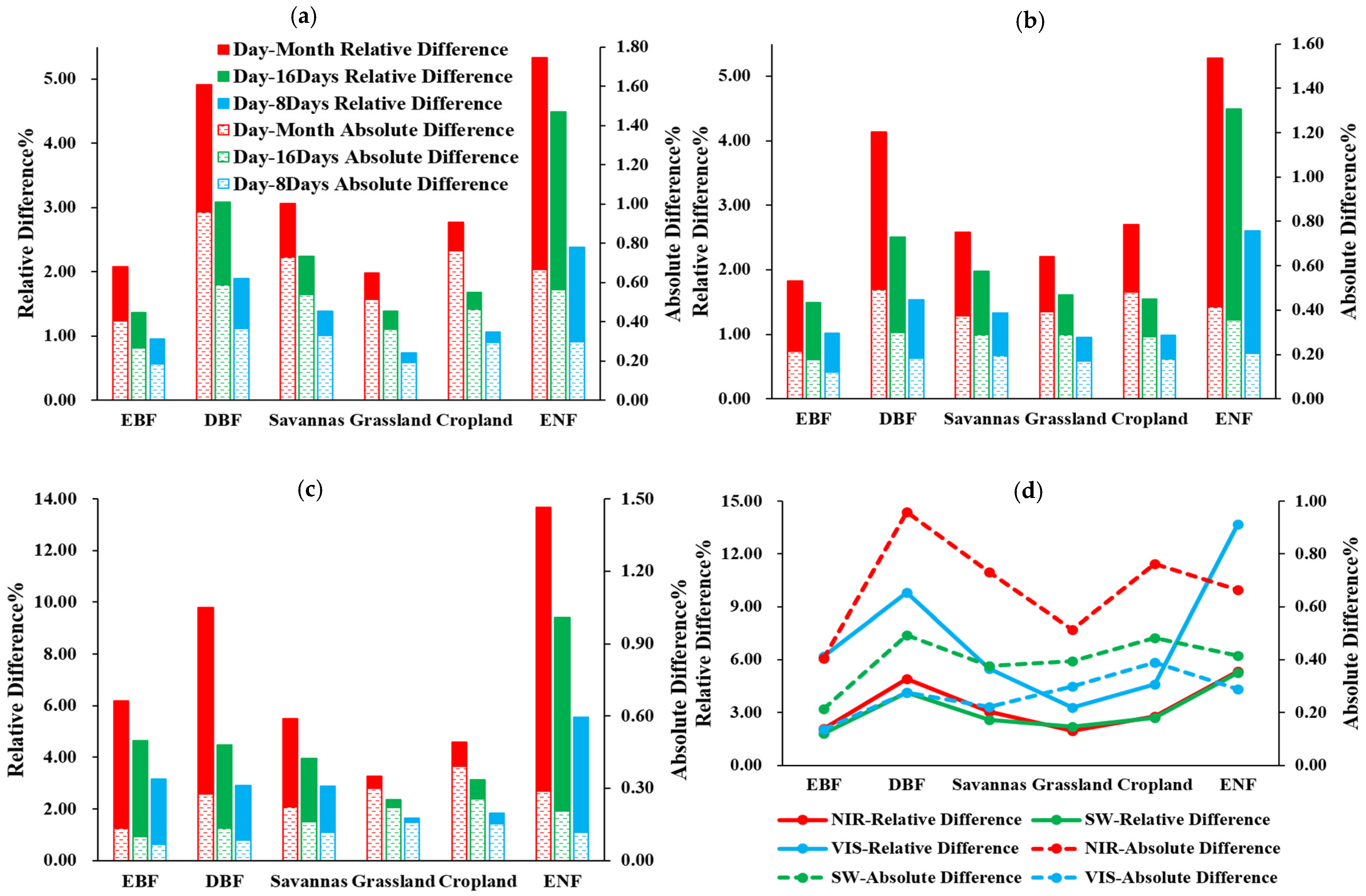
Regarding analysis of albedo differences due to BRDF temporal smoothing, the temporal smoothing of BRDF shows obvious scale effect and seasonality. With the increase in smoothing scale, the albedo differences gradually increase (Figure 11a–c). This conclusion is applicable to the three broad bands (NIR, SW, and VIS) for each study site. Generally, the absolute differences caused by temporal smoothing of BRDF in the NIR band are the largest, while the relative differences in the VIS band are the largest (Figure 11d). This may be related to the biophysical characteristic of vegetation that it needs to absorb light in the VIS band, meanwhile the light in NIR band could be strongly scattered by leaf structure. In addition, the impact of BRDF temporal smoothing shows certain seasonal characteristics, with elevated variation in spring and summer due to the vigorous growth of vegetation (Figure 12d), and limited variation in autumn and winter due to lesser temporal changes over land surface.
The impact of spatial BRDF smoothing on albedo implies certain spectral features accompanied by connections with spatial heterogeneity. The absolute differences caused by spatial BRDF smoothing show the highest values in the NIR band and the highest relative differences in the VIS band (Figure 14). This is consistent with the biophysical characteristics of the vegetation analyzed above, that photosynthesis needs to absorb visible light and produce higher reflectance in the NIR band. Compared with flat grassland, forest effectively increased the differences. In addition, we reconstructed the land surface albedo at 30 m based on Landsat8-OLI images to analyze the spatial heterogeneity of land covers. The results show that the spatial heterogeneity of land cover is related to the albedo differences due to spatial smoothing of BRDF (Figure 15).

6. Conclusions

Several studies have introduced BRDF priori knowledge into albedo retrievals smoothed at different scales. This paper investigated the effects of smoothed BRDF on albedo differences through case studies over six North American regions using operational MODIS-BRDF/Albedo products. Our results show that: (1) as the BRDFs smoothed temporally from daily to monthly, and spatially from 500 m to 5600 m, variations in the magnitude and shapes during BRDF smoothing can be captured, with potential relationships with spectral band, land cover types, and characteristic of vegetation. (2) Temporally smoothed BRDF in NIR, SW, and VIS could lead to apparent relative differences of estimated albedo to smoothed values of 11.3%, 12.5%, and 27.2% and detectable absolute differences of 0.025, 0.012, and 0.013. Further, albedo differences show an obvious seasonal characteristic that differences in spring and summer are significantly higher than those in autumn and winter in the three broadbands. (3) Spatially smoothed BRDF from 500 m to 5.6 km in NIR, SW, and VIS bands could lead to albedo achieving apparent relative differences to smoothed values of 36.5%, 37.1%, and 94.7% and detectable absolute differences of 0.037, 0.024, and 0.018, while albedo differences due to BRDF spatial smoothing are related to heterogeneity of land cover and the overall correlation coefficient between sill values and absolute differences in the three broad bands was 0.8876. The introduction of BRDF priori knowledge of land cover is an important way to produce albedo at high resolution. This work demonstrated that smoothed BRDF after temporal and spatial smoothing can introduce variations in the magnitude and shape of BRDF, and the uncertainty propagating into albedo retrieval is obvious. Thus, it is necessary to avoid the smoothing process in quantitative remote sensing communities, especially when immediate anisotropy retrievals are available at the required spatiotemporal scale.

Author Contributions

Conceptualization, Y.S.; program and process, J.Y.; data organization, J.D.; writing—original draft preparation, J.Y. and Y.S.; writing—review and editing D.X., Q.Z., and R.Z. All authors have read and agreed to the published version of the manuscript.

Funding

This work was supported by the National NSF of China (No. 42071351), the National Key Research and Development Program of China (No. 2020YFA0608501,), the Talent Recruited Program of the Chinese Academy of Science (No. Y938091), Key Laboratory of Land Satellite Remote Sensing Application, Ministry of Natural Resources of China (No. KLSMNR-202107), NSF of Liaoning Province (No. 2020-BS-259), and the Project Supported Discipline Innovation Team of Liaoning Technical University (No. LNTU20TD-23).

Data Availability Statement

Publicly available datasets were analyzed in this study. These datasets can be found here: https://ladsweb.modaps.eosdis.nasa.gov/search/ (accessed on 30 January 2021); https://nassgeodata.gmu.edu/CropScape/ (accessed on 16 February 2021); https://earthexplorer.usgs.gov/ (accessed on 15 August 2021).

Acknowledgments

The authors would like to give thanks to researchers at the Boston University for providing AMBRALS codes.

Conflicts of Interest

The authors declare no conflict of interest.

References

  1. Dickinson, R.E. Land surface processes and climate—Surface albedos and energy balance. In Advances in Geophysics; Elsevier: Amsterdam, The Netherlands, 1983; Volume 25, pp. 305–353. [Google Scholar] [CrossRef]
  2. Pinty, B.; Lavergne, T.; Kaminski, T.; Aussedat, O.; Giering, R.; Gobron, N.; Taberner, M.; Verstraete, M.M.; Voßbeck, M.; Widlowski, J.-L. Partitioning the solar radiant fluxes in forest canopies in the presence of snow. J. Geophys. Res. 2008, 113, D04104. [Google Scholar] [CrossRef] [Green Version]
  3. Lyone, E.A.; Jin, Y.; Randerson, J.T. Changes in surface albedo after fire in boreal forest ecosystems of interior Alaska assessed using MODIS satellite observations. J. Geophys. Res. 2008, 113, G02012. [Google Scholar] [CrossRef] [Green Version]
  4. Ollinger, S.V.; Richardon, A.D.; Martin, M.E.; Hollinger, D.Y.; Frolking, S.E.; Reich, P.B.; Plourde, L.C.; Katul, G.G.; Munger, J.W.; Oren, R.; et al. Canopy nitrogen, carbon assimilation, and albedo in temperate and boreal forests: Functional relations and potential climate feedbacks. Proc. Natl. Acad. Sci. USA 2008, 105, 19336–19341. [Google Scholar] [CrossRef] [PubMed] [Green Version]
  5. Peckham, S.D.; Ahl, D.E.; Serbin, S.P.; Gower, S.T. Fire-induced changes in green-up and leaf maturity of the Canadian boreal forest. Remote Sens. Environ. 2008, 112, 3594–3603. [Google Scholar] [CrossRef]
  6. Yin, J.; Zhan, X.; Zheng, Y.; Christopher, R.; Michael, B.; Wen, J.; Li, F.; Liu, J. Improving Noah land surface model performance using near real time surface albedo and green vegetation fraction. Agric. For. Meteorol. 2016, 218, 171–183. [Google Scholar] [CrossRef]
  7. Li, Y.; Hu, Z. A Preliminary Study on Land-Surface Albedo in Northern Tibetan Plateau. Plateau Meteor. 2006, 25, 1034–1041. [Google Scholar] [CrossRef]
  8. Li, Y.; Zhao, M.; Motesharrei, S.; Mu, Q.; Kalnay, E.; Li, S. Local cooling and warming effects of forests based on satellite observations. Nat. Commun. 2015, 6, 6603. [Google Scholar] [CrossRef] [Green Version]
  9. Chase, T.N.; Pielke, R.A.; Kittel, T.; Nemani, R.R.; Running, S.W. Simulated impacts of historical land cover changes on global climate in northern winter. Clim. Dyn. 2000, 16, 93–105. [Google Scholar] [CrossRef]
  10. Chase, T.N.; Knaff, J.A.; Pielke, R.A.; Kalnay, E. Changes in Global Monsoon Circulations Since 1950. Nat. Hazards 2003, 29, 229–254. [Google Scholar] [CrossRef]
  11. Henderson Sellers, A.; Wilson, M. Surface albedo data for climatic modeling. Rev. Geophys. 1983, 21, 1743–1778. [Google Scholar] [CrossRef]
  12. Jacob, F.; Olioso, A. Derivation of diurnal courses of albedo and reflected solar irradiance from airborne POLDER data acquired near solar noon. J. Geophys. Res. 2005, 110, D10104. [Google Scholar] [CrossRef]
  13. Sellers, P.; Meeson, B.; Hall, F.; Asrar, G.; Murphy, R.; Schiffer, R.; Bretherton, F.; Dickinson, R.; Ellingson, R.; Field, C. Remote sensing of the land surface for studies of global change: Models-Algorithms-Experiments. Remote Sens. Environ. 1995, 51, 3–26. [Google Scholar] [CrossRef]
  14. Alton, P.B. A simple retrieval of ground albedo and vegetation absorptance from MODIS satellite data for parameterisation of global Land-Surface Models. Agric. For. Meteorol. 2009, 149, 1769–1775. [Google Scholar] [CrossRef]
  15. Mira, M.M.; Frédéric, B.; Dominique, C.; Olivier, H.; Belen, G.; Albert, O. The MODIS (collection V006) BRDF/albedo product MCD43D: Temporal course evaluated over agricultural landscape. Remote Sens. Environ. 2015, 170, 216–228. [Google Scholar] [CrossRef] [Green Version]
  16. Jacob, F.; Olioso, A.; Gu, X.F.; Su, Z.B.; Seguin, B. Mapping surface fluxes using airborne visible, near infrared, thermal infrared remote sensing data and a spatialized surface energy balance model. Agronomie 2002, 22, 669–680. [Google Scholar] [CrossRef]
  17. Hollinger, D.; Ollinger, S.V.; Richardson, A.D.; Meyers, T.P.; Dail, D.B.; Martin, M.E.; Scott, N.A.; Arkebauer, T.J.; Baldocchi, D.D.; Clark, K.L.; et al. Albedo estimates for land surface models and support for a new paradigm based on foliage nitrogen concentration. Glob. Chang. Biol. 2010, 16, 696–710. [Google Scholar] [CrossRef] [Green Version]
  18. Deschamps, P.Y.; Bréon, F.M.; Leroy, M.; Podaire, A.; Bricaud, A.; Buriez, J.C.; Seze, G. The POLDER mission: Instrument characteristics and scientific objectives. IEEE Trans. Geosci. Remote Sens. 1994, 32, 598–615. [Google Scholar] [CrossRef]
  19. Masuoka, E.; Fleig, A.; Wolfe, R.; Patt, F. Key characteristics of MODIS data products. IEEE Trans. Geosci. Remote Sens. 1998, 36, 1313–1323. [Google Scholar] [CrossRef]
  20. Diner, D.J.; Beckert, J.C.; Reilly, T.H.; Bruegge, C.; Conel, J.; Kahn, R.; Martonchik, J.; Ackerman, T.; Davies, R.; Gerstl, S.; et al. Multiangle Imaging Spectro Radiometer (MISR) description and experiment overview. IEEE Trans. Geosci. Remote Sens. 1998, 36, 1072–1087. [Google Scholar] [CrossRef]
  21. Bréon, F.M.; Maignan, F. A BRDF–BPDF database for the analysis of earth target reflectances. Earth Syst. Sci. Data 2017, 9, 31–45. [Google Scholar] [CrossRef] [Green Version]
  22. Lucht, W.; Schaaf, C.; Strahler, A. An algorithm for the retrieval of albedo from space using semiempirical BRDF models. IEEE Trans. Geosci. Remote Sens. 2000, 38, 977–998. [Google Scholar] [CrossRef] [Green Version]
  23. Bruegge, C.; Chrien, N.L.; Haner, D. A Spectralon BRF data base for MISR calibration applications. Remote Sens. Environ. 2001, 77, 354–366. [Google Scholar] [CrossRef]
  24. Kimes, D.S.; Sellers, P.J. Inferring hemispherical reflectance of the earth’s surface for global energy budgets from remotely sensed nadir or directional radiance values. Remote Sens. Environ. 1985, 18, 205–223. [Google Scholar] [CrossRef]
  25. Kimes, D.S.; Sellers, P.J.; Newcomb, W.W. Hemispherical Reflectance Variations of Vegetation Canopies and Implications for Global and Regional Energy Budget Studies. J. Clim. Appl. Meteorol. 1987, 26, 959–972. [Google Scholar] [CrossRef] [Green Version]
  26. Nicodemus, F.E.; Richmond, J.C.; Hsia, J.J.; Ginsberg, I.W.; Limperis, T. Geometrical Considerations and Nomenclature for Reflectance; National Bureau of Standards: Washington, DC, USA, 1977; pp. 1–50. [Google Scholar] [CrossRef]
  27. Song, F.; Fan, W.; Liu, Q.; Xu, X. A Method of Acquiring BRDF of Objects in the Field. J. Remote Sens. 2007, 11, 296–302. [Google Scholar]
  28. Zhu, G.L.; Ju, W.M.; Chen, J.M.; Liu, Y.B.; Zhu, J.F.; Xing, B.L. Validation of MODIS BRDF model parameters product and the Ross-Li model with POLDER data. J. Remote Sens. 2011, 15, 875–894. [Google Scholar] [CrossRef]
  29. He, D.D.; Jiao, Z.T.; Dong, Y.D.; Zhang, X.N.; Ding, A.X.; Yin, S.Y.; Cui, L.; Chang, Y.X. Preliminary verification of Landsat satellite albedo from airborne WIDAS data. J. Remote Sens. 2019, 23, 53–61. [Google Scholar] [CrossRef]
  30. Wanner, W.; Li, X.; Strahler, A.H. On the derivation of kernels for kernel-driven models of bidirectional reflectance. J. Geophys. Res. Atmos. 1995, 100, 21077–21089. [Google Scholar] [CrossRef]
  31. Roujean, J.L.; Leroy, M.; Deschamps, P.Y. A bidirectional reflectance model of the Earth’s surface for the correction of remote sensing data. J. Geophys. Res. Atmos. 1992, 97, 20455–20468. [Google Scholar] [CrossRef]
  32. Roujean, J.L.; Tanré, D.; Bréon, F.M.; Deuzé, J.-L. Retrieval of land surface parameters from airborne POLDER bidirectional reflectance distribution function during HAPEX-Sahel. J. Geophys. Res. Atmos. 1997, 102, 11201–11218. [Google Scholar] [CrossRef]
  33. Bacour, C.; Bréon, F.M. Variability of biome reflectance directional signatures as seen by POLDER. Remote Sens. Environ. 2005, 98, 80–95. [Google Scholar] [CrossRef]
  34. Schaaf, C.; Gao, F.; Strahler, A.; Lucht, W.; Li, X.; Tsang, T.; Strugnell, N.; Zhang, X.; Jin, Y.; Muller, J. First operational BRDF, albedo nadir reflectance products from MODIS. Remote Sens. Environ. 2002, 83, 135–148. [Google Scholar] [CrossRef] [Green Version]
  35. Shuai, Y.; Masek, J.; Gao, F.; Schaaf, C. An algorithm for the retrieval of 30-m snow-free albedo from Landsat surface reflectance and MODIS BRDF. Remote Sens. Environ. 2011, 115, 2204–2216. [Google Scholar] [CrossRef]
  36. Shuai, Y.; Masek, J.; Gao, F.; Schaaf, C.; He, T. An Approach for the Long-Term 30-m Land Surface Snow-Free Albedo Retrieval from Historic Landsat Surface Reflectance and MODIS-based a Priori Anisotropy Knowledge. Remote Sens. Environ. 2014, 152, 467–479. [Google Scholar] [CrossRef]
  37. Franch, B.; Vermote, E.; Claverie, M. Intercomparison of Landsat albedo retrieval techniques and evaluation against in situ measurements across the US SURFRAD network. Remote Sens. Environ. 2014, 152, 627–637. [Google Scholar] [CrossRef]
  38. Vermote, E.; Justice, C.; Bréon, F. Towards a Generalized Approach for Correction of the BRDF Effect in MODIS Directional Reflectances. IEEE Trans. Geosci. Remote Sens. 2009, 47, 898–908. [Google Scholar] [CrossRef]
  39. Jiao, Z.; Zhang, H.; Li, X. To derive a prior database of archetypal BRDF shapes from ground measurements using anisotropic flat index (AFX). In Proceedings of the 2012 IEEE International Geoscience and Remote Sensing Symposium, Munich, Germany, 22–27 July 2012; pp. 6753–6756. [Google Scholar] [CrossRef]
  40. Jiao, Z.; Michael, J.H.; Crystal, S.; Zhang, H.; Wang, Z.; Li, X. An Anisotropic Flat Index (AFX) to derive BRDF archetypes from MODIS. Remote Sens. Environ. 2014, 141, 168–187. [Google Scholar] [CrossRef]
  41. Zhang, H.; Jiao, Z.; Dong, Y.D.; Huang, X.Y.; Li, J.Y.; Li, X.W. An algorithm for retrieval albedo from BRDF archetype. J. Remote Sens. 2013, 17, 1475–1491. [Google Scholar] [CrossRef]
  42. Friedl, M.; McIver, D.; Hodges, J.; Zhang, X.; Muchoney, D.; Strahler, A.; Woodcock, C.; Gopal, S.; Schneider, A.; Cooper, A.; et al. Global land cover mapping from MODIS: Algorithms and early results. Remote Sens. Environ. 2002, 83, 287–302. [Google Scholar] [CrossRef]
  43. Friedl, M.A.; Sulla-Menashe, D.; Tan, B.; Schneider, A.; Ramankutty, N.; Sibley, A.M.; Huang, X. MODIS Collection 5 global land cover: Algorithm refinements and characterization of new datasets. Remote Sens. Environ. 2010, 114, 168–182. [Google Scholar] [CrossRef]
  44. Loveland, T.; Belward, A. The IGBP-DIS global 1km land cover data set, DISCover: First results. Int. J. Remote Sens. 1997, 18, 3289–3295. [Google Scholar] [CrossRef]
  45. Loveland, T.R.; Reed, B.C.; Brown, J.F.; Ohlen, D.O.; Zhu, Z.; Yang, L.; Merchant, J.W. Development of a global land cover characteristics database and IGBP DISCover from 1 km AVHRR data. Int. J. Remote Sens. 2000, 21, 1303–1330. [Google Scholar] [CrossRef]
  46. Boryan, C.; Yang, Z.; Mueller, R.; Craig, M. Monitoring US agriculture: The US Department of Agriculture, National Agricultural Statistics Service, Cropland Data Layer Program. Geocarto Int. 2011, 26, 341–358. [Google Scholar] [CrossRef]
  47. Wickham, J.D.; Stehman, S.V.; Gass, L.; Dewitz, J.; Sorenson, D.G.; Granneman, B.; Poss, R.V.; Baer, L.A. Thematic accuracy assessment of the 2011 National Land Cover Database (NLCD). Remote Sens. Environ. 2017, 191, 328–341. [Google Scholar] [CrossRef] [Green Version]
  48. Roy, D.P.; Wulder, M.A.; Loveland, T.R.; Woodcock, C.E.; Allen, R.G.; Anderson, M.C.; Helder, D.; Irons, J.R.; Johnson, D.M.; Kennedy, R.; et al. Landsat-8: Science and Product Vision for Terrestrial Global Change Research. Remote Sens. Environ. 2014, 145, 154–172. [Google Scholar] [CrossRef] [Green Version]
  49. Wolfe, R.; Roy, D.; Vermote, E. MODIS land data storage, gridding, and compositing methodology: Level 2 grid. IEEE Trans. Geosci. Remote Sens. 1998, 36, 1324–1338. [Google Scholar] [CrossRef] [Green Version]
  50. Yang, K.; Wolfe, R. MODIS level 2 grid with the ISIN map projection. In Proceedings of the IEEE 2001 International Geoscience and Remote Sensing Symposium, Sydney, Australia, 9–13 July 2001; pp. 3291–3293. [Google Scholar] [CrossRef]
  51. Gao, F. MODIS bidirectional reflectance distribution function and albedo Climate Modeling Grid products and the variability of albedo for major global vegetation types. J. Geophys. Res. Atmos. 2005, 110, D01104. [Google Scholar] [CrossRef] [Green Version]
  52. Wanner, W.; Strahler, A.H.; Hu, B.; Lewis, P.; Muller, J.P.; Li, X.; Barker Schaaf, C.L.; Barnsley, M.J. Global retrieval of bidirectional reflectance and albedo over land from EOS MODIS and MISR data: Theory and algorithm. J. Geophys. Res. 1997, 102, 17143–17162. [Google Scholar] [CrossRef] [Green Version]
  53. Zheng, Y.H.; Huang, L.; Zhai, J. Impacts of land cover changes on surface albedo in China, the United States, India and Brazil. J. Remote Sens. 2020, 24, 917–932. [Google Scholar] [CrossRef]
  54. Zhang, H.; Jiao, Z.T.; Dong, Y.D.; Li, J.Y.; Li, X.W. Albedo retrieved from BRDF archetype and surface directional reflectance. Remote Sens. 2015, 19, 355–367. [Google Scholar] [CrossRef]
  55. Susaki, J.; Yasuoka, Y.; Kajiwara, K.; Honda, Y.; Hara, K. Validation of MODIS Albedo Products of Paddy Fields in Japan. IEEE Trans. Geosci. Remote Sens. 2006, 45, 206–217. [Google Scholar] [CrossRef]
  56. Miguel, O.R.; Schaaf, C.B.; Woodcock, C.E.; Strahler, A.H.; Yang, X.; Braswell, B.; Curtis, P.S.; Davis, K.J.; Dragoni, D.; Goulden, M. The MODIS (Collection V005) BRDF/albedo product: Assessment of spatial representativeness over forested landscapes. Remote Sens. Environ. 2009, 113, 2476–2498. [Google Scholar] [CrossRef] [Green Version]
  57. Wang, Z.; Schaaf, C.B.; Chopping, M.J.; Strahler, A.H.; Wang, J.; Román, M.; Rocha, A.V.; Woodcock, C.E.; Shuai, Y. Evaluation of Moderate-resolution Imaging Spectroradiometer (MODIS) snow albedo product (MCD43A) over tundra. Remote Sens. Environ. 2012, 117, 264–280. [Google Scholar] [CrossRef]
  58. Jiao, Z.; Dong, Y.; Schaaf, C.B.; Chen, J.M.; Román, M.; Wang, Z.; Zhang, H.; Ding, A.; Erb, A.; Hill, M.; et al. An algorithm for the retrieval of the clumping index (CI) from the MODIS BRDF product using an adjusted version of the kernel-driven BRDF model. Remote Sens. Environ. 2018, 209, 594–611. [Google Scholar] [CrossRef]
  59. Liang, S. Narrowband to Broadband Conversions of Land Surface Albedo I: Algorithms. Remote Sens. Environ. 2001, 76, 213–238. [Google Scholar] [CrossRef]
  60. Wang, Z.S.; Erb, A.; Schaaf, C.; Sun, Q.; Liu, Y.; Yang, Y.; Shuai, Y.; Casey, K.; Roman, M. Early spring post-fire snow albedo dynamics in high latitude boreal forests using Landsat-8 OLI data. Remote Sens. Environ. 2016, 185, 71–83. [Google Scholar] [CrossRef] [Green Version]
  61. Huete, A.; Didan, K.; Miura, T.; Rodriguez, E.P.; Gao, X.; Ferreira, L.G. Overview of the radiometric and biophysical performance of the MODIS vegetation indices. Remote Sens. Environ. 2002, 83, 195–213. [Google Scholar] [CrossRef]
  62. Liu, H.Q.; Huete, A. A feedback based modification of the NDVI to minimize canopy background and atmospheric noise. IEEE Trans. Geosci. Remote Sens. 1995, 33, 457–465. [Google Scholar] [CrossRef]
  63. Gao, B. NDWI—A normalized difference water index for remote sensing of vegetation liquid water from space. Remote Sens. Environ. 1996, 58, 257–266. [Google Scholar] [CrossRef]
  64. Gao, F.; Schaaf, C.B.; Strahler, A.H.; Jin, Y.; Li, X. Detecting Vegetation Structure using a Kernel-based BRDF Model. Remote Sens. Environ. 2003, 86, 198–205. [Google Scholar] [CrossRef]
  65. Wang, Q.; Ni-Meister, W. Forest Canopy Height and Gaps from Multiangular BRDF, Assessed with Airborne LiDAR Data. Remote Sens. 2019, 11, 2566. [Google Scholar] [CrossRef] [Green Version]
  66. Wu, S.; Wen, J.; Liu, Q.; You, D.; Yin, G.; Lin, X. Improving Kernel-Driven BRDF Model for Capturing Vegetation Canopy Reflectance with Large Leaf Inclinations. IEEE J. Sel. Top. Appl. Earth Obs. Remote Sens. 2020, 13, 2639–2655. [Google Scholar] [CrossRef]
Figure 1. The distributions of land cover types at 500 m for each study site within MODIS pixels (5600 m).
Remotesensing 14 02001 g001
Figure 2. The proportion of categories in MODIS pixels (5600 m and 500 m) for each study site based on CDL (first three categories).
Remotesensing 14 02001 g002
Figure 3. Diagram of smoothing BRDF/Albedo in multi-spatiotemporal scales. (a) Smoothing in temporal scales; (b) Smoothing in spatial scales.
Remotesensing 14 02001 g003
Figure 4. The Workflow chart.
Remotesensing 14 02001 g004
Figure 5. Schematic diagram of the BRDF principal plane and characteristic directions in the principal plane. (a) Principal plane of BRDF; (b) Characteristic directions of principle plane.
Remotesensing 14 02001 g005
Figure 6. The distribution of daily vegetation index (EVI) and seasonal statistics of EVI for each selected study site. (a) Vegetation index; (b) Statistics of seasonal EVI.
Remotesensing 14 02001 g006
Figure 7. Semi-variogram curves and Landsat-8 OLI images (Savanna, band 7–5–3). (a) Semi-variogram (Savanna, DOY 205); (b) Semi-variogram (Savanna, DOY 365); (c) Landsat-8 bands 7–5–3 (Savannas, DOY 205); (d) Landsat-8 bands 7–5–3 (Savanna, DOY 365).
Remotesensing 14 02001 g007
Figure 8. Comparison of smoothed BRDF in the principal plane with the daily retrievals over selected EBF (a), DBF (b), Savanna (c), Grassland (d), Cropland (e), and ENF (f) sites in June of 2019.
Remotesensing 14 02001 g008
Figure 9. Statistics of magnitude difference and standard deviation of BRDF principal planes due to BRDF temporal smoothing in 2019/06 (a,b) and their annual average level for each study site (c,d).
Remotesensing 14 02001 g009
Figure 10. Comparison of smoothed BRDF principal plane at 5600 m with the retrievals at 500 m within three broadbands on the extreme DOYs for ENF (a) and Grassland (b).
Remotesensing 14 02001 g010
Figure 11. Statistics of albedo differences due to BRDF temporal smoothing in NIR (a), SW (b), VIS (c) and the average monthly albedo differences (d) for each study site.
Remotesensing 14 02001 g011
Figure 12. Statistics of the seasonal distribution for monthly albedo differences in NIR (a), SW (b), VIS (c) and the comprehensive data for each season based on each study site (d).
Remotesensing 14 02001 g012
Figure 13. Daily variation curves of albedo due to BRDF spatial smoothing in three broad bands for each selected EBF (a), DBF (b), Savanna (c), Grassland (d), Cropland (e), and ENF (f) site.
Remotesensing 14 02001 g013
Figure 14. Statistics of albedo differences due to BRDF spatial smoothing at annual level for each site in three broad bands.
Remotesensing 14 02001 g014
Figure 15. The Relationship of sill values with albedo differences (a) and albedo RMSE (b).
Remotesensing 14 02001 g015
Table 1. Statistics of Study Sites.
SiteConfidence (%)Altitude (m)Slope (°)Longitude (°)Latitude (°)Climate Zone
ENF92312416.42−105.5839.68Mountain climate
CropLand9710741.39−101.9837.73Temperate continental climate
Grassland9612762.02−102.6336.43Temperate continental climate
Savannas89832.58−95.7831.38Subtropical climate
DBF93602.84−94.8831.23Subtropical climate
EBF98432.47−93.5830.58Subtropical climate
Note: EBF denotes evergreen broadleaf forests, DBF for deciduous broadleaf forests, and ENF for evergreen needleleaf forests.
Table 2. Statistics of MODIS data sets.
NumberNameResolutionProjectionFunction
1MCD12C15600 mLongitude and latitudeClassification information in 5600 m
2MCD12Q1500 mSinusoidalClassification information in 500 m
3MCD43C15600 mLongitude and latitudeParameters of BRDF in 5600 m
4MCD43C35600 mLongitude and latitudeAlbedo in 5600 m
5MCD43A1500 mSinusoidalParameters of BRDF in 500 m
6MCD43A3500 mSinusoidalAlbedo in 500 m
7MCD43A4500 mSinusoidalObservations of zenith directions
Table 3. Statistics of semi-variogram parameters for each study site.
SiteStationDOYNIRSWVIS
C0 (10−6)C (10−6)A (m)C0 (10−6)C (10−6)A (m)C0 (10−6)C (10−6)A (m)
EBFleaf-on2071085446904924769020112690
leaf-on3197221851026107540773660
DBFleaf-on862761590135082555135013115960
leaf-off358301175013801138031380252931350
Savannasleaf-on2052491226990844541020271281050
leaf-off365329219611701289711140373201200
Croplandleaf-on192123246496080132410507011281140
leaf-off352142319814108016761500468421200
Grasslandleaf-on17663347105041199105023951050
leaf-off352756571560443581560201341560
ENFleaf-on24711513061020535391020201251050
leaf-on27715820151110768731110272081080
Table 4. Differences in BRDF principal planes due to spatial smoothing for ENF and Grassland in extreme DOYs.
SiteBandDOYMagnitude (%)HotSpot (%)−45° (%)−70° (%)+45° (%)+70° (%)Zenith (%)SD
ENFNIR1761.573.481.124.493.378.022.002.20
SW1800.851.590.682.251.523.620.960.97
VIS1800.390.790.311.20.721.870.480.52
GrasslandNIR1520.861.191.211.790.911.720.910.35
SW1530.370.740.631.090.621.080.550.22
VIS2600.290.650.380.830.460.740.530.16
Table 5. Extreme monthly differences in albedo due to BRDF temporal smoothing in all study sites.
BandRelative DifferenceAbsolute Difference
Maximum (%)SiteMonthMaximumSiteMonth
NIR11.3ENF60.025Cropland3
SW12.5ENF60.012Grassland5
VIS27.2DBF70.013Cropland6
Table 6. Maximum daily albedo differences due to BRDF spatial smoothing for each study site.
SiteBandDOYAbsolute DifferenceDOYRelative Difference (%)
ENFVIS3050.01818094.7
NIR1760.03717636.5
SW1760.02418037.1
CroplandVIS1260.01712618.5
NIR1250.0341114.1
SW110.0201113.2
GrasslandVIS1220.0091229.41
NIR1220.0181226.49
SW1220.0111226.12
SavannasVIS970.01021720.8
NIR1010.027611.8
SW1010.015610.1
DBFVIS920.00915827.2
NIR1340.0303317.4
SW1340.0173214.4
EBFVIS1990.00919983.8
NIR650.0296513.8
SW650.0206515.0
Publisher’s Note: MDPI stays neutral with regard to jurisdictional claims in published maps and institutional affiliations.

