Abstract
Warmer or cooler spring in northern high latitudes will, for the most part, directly impact gross primary productivity (GPP) of ecosystems, but also carry consequences for the upcoming seasonal GPP. Spatiotemporal patterns of these legacy effects are still largely unknown but important for improving our understanding of how plant phenology is associated with vegetation dynamics. In this study, impacts of spring temperature anomalies on spring, summer and autumn GPP were investigated, and the dominant drivers of summer and autumn GPP including air temperature, vapor pressure deficit and soil moisture have been explored for northern ecosystems (>30°N). Three remote sensing products of seasonal GPP (GOSIF-GPP, NIRv-GPP and FluxSat-GPP) over 2001–2018, all based on a spatial resolution of 0.05°, were employed. Our results indicate that legacy effects from spring temperature are most pronounced in summer, where they have stimulating effects on the Arctic ecosystem productivity. Spring warming likely lessens the harsh climatic constraints that govern the Arctic tundra and extends the growing season length. Further south, legacy effects are mainly negative. This strengthens the hypothesis that enhanced vegetation growth in spring will increase plant water demand and stress in summer and autumn. Soil moisture is the dominant control of summer GPP in temperate regions. However, the dominant meteorological variables controlling vegetation growth may differ depending on the GPP products, highlighting the need to address uncertainties among different methods of estimating GPP.
1. Introduction
The last decades have seen a rapid increase in global temperatures, particularly more pronounced in the northern high latitudes [1]. The rapid warming may lead to changes in the timing of thermal growing seasons and phenological cycles of plants [2]. Earlier onsets of spring, increased frequency of droughts as well as changing precipitation patterns have been observed [1]. These changes may induce direct and legacy effects on ecosystem gross primary production (GPP—the gross uptake of carbon dioxide (CO) by plant photosynthesis) as well as various types of climate feedback associated with ecosystem responses to climatic warming [3,4].
Direct impacts on growing-season vegetation productivity due to seasonal warming or drought have been studied previously [5,6]. Spring warming directly affects the onset of leaf growth by advancing bud-burst, leading to increases in spring GPP () and a generally earlier greening of vegetation [7,8]. Summer warming may have positive effects on Arctic and alpine biomes. Based on annual shrub ring-width measurements and long-term meteorological records, growth of both evergreen and deciduous dwarf shrubs were found to be stimulated due to summer warmth [9]. However, severe and long-lasting warming events, i.e., heat waves, may dampen vegetation productivity due to soil moisture deficits, or reach the thermal tolerance threshold of photosynthetic decline in forest growth [10,11]. Similarly, autumn warming can enhance photosynthesis rates via the delayed senescence of plants, however, soil decomposition can also increase, leading to net carbon losses of the ecosystems during this season [12].
Nevertheless, the legacy effects of spring temperature () anomalies on seasonal GPP is known to a lesser degree. Currently, even the state-of-the-art terrestrial biosphere models struggle to implement them [3]. As noted by [5], most carbon-cycle models seem to overestimate the positive legacy effects on GPP caused by spring warming and underestimate the potential influence of built-up water stress. Accurately assessing direct and legacy effects of seasonal warming on vegetation productivity is important, as vegetation is a key component of the global carbon, water and energy cycles, and its responses may trigger biogeochemical and biophysical climate feedback [13]. A proper understanding of these highly dynamic systems is crucial, particularly for our general ability to accurately predict and mitigate climate impacts, as well as adapting our society to a changing climate [14].
Recent works [5,6,15] indicate that annual GPP can be suppressed or stimulated by both cooler and warmer springs. For example, boreal forests have seen a dampening effect on peak summer productivity related to early springs [16,17]. The suppressed vegetation productivity in summer can be caused by soil moisture deficits resulting from winter precipitation and early onset of vegetation. Other northern ecosystems, mainly dominated by graminoids, lichens and deciduous shrubs, have been shown to benefit from a fairly early date of snowmelt, as many such species are unable to accelerate or adapt their rate of phenological development [18,19]. The delayed outcome, or carry-over effect, thus depends on a combination of several factors, including meteorological and environmental conditions, vegetation composition and phenological responses of vegetation, but as of now, a comprehensive understanding of how these factors interplay remains lacking. Earlier research in this area has attempted to address these questions utilizing data sets with relatively coarse resolution (50 × 50 km) based on the Normalized Difference Vegetation Index (NDVI) (e.g., [10,16]). As vegetation response to warming is spatially non-uniform, such a coarse resolution may fail to represent explicit details of greening and browning trends of different ecosystems. Moreover, NDVI is often claimed to misrepresent the non-linear nature of vegetation responses, and is thus regarded as less efficient to be a proxy of GPP [20,21].
Recently, a few novel products have been tested and regarded as more robust proxies for canopy structure, leaf pigment content, and, subsequently, plant photosynthetic potential. Among these products, GOSIF (Global Orbiting Carbon Observatory-2 Solar-Induced Chlorophyll Fluorescence data set)-GPP, NIRv (Near-Infrared Reflectance of terrestrial vegetation)-GPP and FluxSat (Fluxnet data fused with satellite images)-GPP, based on Solar-Induced chlorophyll Fluorescence (SIF), canopy near-infrared reflectance, eddy flux and satellite data fusion, respectively, are shown to better reflect photosynthetic activities [22,23,24,25]. In this study, we have utilized these three products, and the approach of each product is distinctly different from the others. Based on a higher spatial resolution (0.05°), we aim to explore the direct and legacy effects of spring temperature anomalies on seasonal GPP with greater detail and accuracy.
We have hypothesized that direct and legacy effects of spring warming or cooling, will either stimulate or suppress GPP in summer, autumn or across both seasons. This, in turn, depends on amplified or dampened water stress, the sensitivity of plant species to summer warmth and biological conditions of spring. The summer response of GPP can further affect the autumn phenology by advancing or delaying the senescence of plants. Therefore, the main aims are to answer the following questions: (1) What are the geographical distribution and patterns of direct and lagged responses of GPP to spring temperature anomalies? (2) How does each biome respond to these direct and lagged effects? (3) How do the dominant drivers (environmental variables, current and pre-seasonal GPP) explain summer and autumnal GPP? For environmental variables, this study only considers warming and drought-related variables, that is, temperature, soil moisture and vapor pressure deficit (VPD).
2. Materials and Methods
2.1. Study Area and Biome Classification
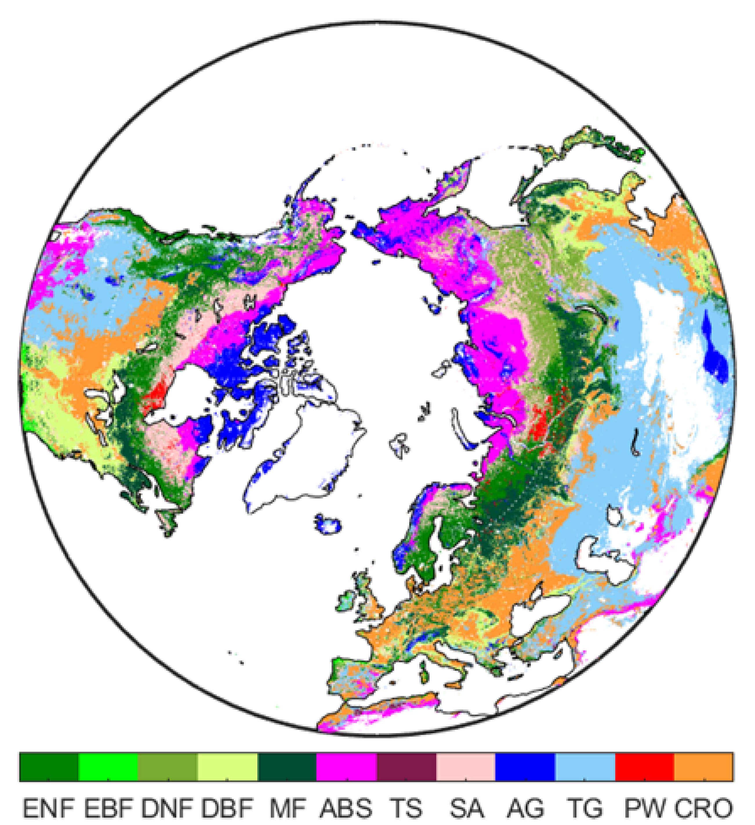
The study area covers land areas (∼41 million km) located north of 30N, encompassing several land cover types from the Arctic/subarctic tundra in the high latitudes to temperate forests and grasslands in the south. Regions located north of 30N have manifested a strong seasonality for climatic thermal conditions and vegetation productivity in the growing season. To make our results comparable to many other studies, the seasons were defined as: spring (March, April, and May), summer (June, July, and August) and autumn (September, October, and November). The biome classification used in this study was based on the global land cover data set from the Terra and Aqua Combined Moderate Resolution Imaging Spectroradiometer (MODIS) Land Cover Climate Modeling Grid (MCD12C1) Version 6 Yearly L3 Product [26] and the Köppen–Geiger climate map (1 × 1 km) of the world [27,28] for the year 2011. The MODIS land cover data set uses the biome classification scheme of the International Geosphere-Biosphere Programme (IGBP), which was to generate 17 land classes to meet the needs of the IGBP core science projects relevant to climate, carbon cycle, and others [29]. To separate alpine and high arctic tundra from low-laying temperate grasslands or shrublands, the MODIS grasslands were divided into temperate and arctic grasslands and the MODIS shrublands were divided into temperate and arctic and boreal shrublands. Overall, there are 12 terrestrial biomes that were included in the study area: evergreen needleleaf forests (ENF), evergreen broadleaf forests (EBF), deciduous needleleaf forests (DNF), deciduous broadleaf forests (DBF), mixed forests (MF), arctic and boreal shrublands (ABS), temperate shrublands (TS), savanna (SV), arctic grasslands (AG), temperate grasslands (TG), permanent wetlands (PW), and croplands (CRO) (Figure A1). A more thorough description of each biome type is given in Table 1.

Table 1.
Definitions of the 12 terrestrial biomes were developed by [26]. Grass- and shrublands were further divided in Arctic/boreal and temperate groups according to [27,28].
2.2. Data Sets of Gross Primary Productivity
All three GPP data sets used in this study can be retrieved freely from the links listed in the Data Availability Statement, and also viewed in Table 2. The time-span of the analysis (2001–2018) was confined by the availability of the NIRv-GPP product, which has only been processed to the year 2018.
2.2.1. GOSIF-GPP
The monthly GOSIF-GPP product (2001–2018) used in this study is generated based on a global SIF data set from the Orbiting Carbon Observatory-2 (OCO-2) (i.e., GOSIF) and its biome-specific linear relationship with the measured GPP [30]. The GOSIF-GPP data set was estimated using a data-driven model, in which variables reflecting vegetation conditions, meteorological conditions, and land cover information were used as model input [31]. It is based on SIF observations made by NASA’s sun-synchronous and polar Orbiting Carbon Observatory-2 (OCO-2) (launched 2014). SIF retrieved by OCO-2 has a higher resolution (1.3 × 2.25 km) and data acquisition rate compared to, e.g., GOSAT or Global Ozone Monitoring Experiment (GOME). These measurements are still too spatially sparse to provide a data set with (spatial) resolution over a long-term period. The authors of [30] used eight biome-specific linear relationships between SIF and GPP, in combination with machine-learning techniques to create a global coverage () of SIF-based GPP from the year 2001 to 2018. Climate data, such as air temperature, photosynthetic active radiation (PAR), and VPD, was used in combination with the Enhanced Vegetation Index (EVI) retrieved from MODIS MCD43C4v006 to help with calibration of SIF. Compared to GPP retrieved from Eddy Covariance (EC) measurements of 91 sites (https://fluxnet.org/data/fluxnet2015-dataset/, accessed on 6 March 2022, FLUXNET tier1) an overall correlation coefficient (R) between EC measurements and GOSIF-GPP is ().
2.2.2. NIRv-GPP
The monthly global NIRv-GPP data set was derived based on the Advanced Very High Resolution Radiometer (AVHRR) reflectance from LTDR (Land Long Term Data Record v4) product [24]. NIRv is the product of total scene near-infrared reflectance (NIR) and NDVI, commonly used as a proxy to represent vegetation productivity [23]. Based on the established linear relationship between NIRv and EC flux-derived GPP from 104 flux towers, the global monthly 0.05 of GPP data set was estimated. This approach yielded a mean , around 0.70, for the validation sites. The NIRv-GPP data set uses no climate data as input.
2.2.3. FluxSat-GPP
The third data set of monthly global GPP (0.05°) was derived based on the MODIS MCD43C4v006 Nadir Bidirectional Reflectance Distribution Function-Adjusted Reflectance (NBAR) product, SIF, PAR, plant and soil classification data, FLUXNET GPP, meteorological and hydrological fields. These data sets were used as input to a neural-network model to estimate GPP on a global scale [25].
Table 2.
Main data sets used in the study. Bilinear interpolation was used to convert the ERA5land climate data from to . The time-span of the analysis (2001–2018) was confined by the availability of the GPP-data products.
Table 2.
Main data sets used in the study. Bilinear interpolation was used to convert the ERA5land climate data from to . The time-span of the analysis (2001–2018) was confined by the availability of the GPP-data products.
| Name | Spatial | Temporal | Time Span | Data Source |
|---|---|---|---|---|
| GOSIF-GPP | 0.05 | monthly | 2001–2018 | [30] |
| NIRv-GPP | 0.05 | monthly | 2001–2018 | [24] |
| FluxSat-GPP | 0.05 | monthly | 2001–2018 | [25] |
| MODIS land cover (MCD12C1 v006) | 0.05 | yearly | 2011 | [26] |
| the Köppen–Geiger climate map | 1 km | static | 2007 | [27,28,32] |
| ERA5-land (air temperature, soil moisture and VPD) | 0.1 | monthly | 2001–2018 | [33] |
2.3. ERA5-Land Air Temperature, Soil Moisture and Vapor Pressure Deficit
ERA5-Land is the high-resolution land component product based on the fifth generation of the European ReAnalysis (ERA5) data set, which is used as forcing to drive the European Centre for Medium-Range Weather Forecasts (ECMWF) land surface model [33]. It provides a consistent view of the evolution of land variables over several decades at an enhanced resolution (9 km) compared to the reanalysis products such as ERA5 (31 km) and ERA-Interim (80 km). The added values of ERA5-land consist of improved representation of hydrological cycle, including soil moisture, river discharge and lake description [33]. We used 2 m air temperature, 2 m dew-point temperature, soil moisture (0–7 cm), and surface pressure from the ERA5-land product. VPD was calculated based on 2 m air and dew-point temperature and surface pressure [34].
2.4. Pre-Treatment of the Data
The spatial resolution of all the data sets in this study needs to be aligned and compatible to be able to produce viable correlations. The spatial scale chosen for this study is , and data with a lower resolution thus needs to be converted. This conversion was performed using bilinear interpolation. The spatial resolution (0.05), that each pixel covers varies across the study-area, and mainly depends on the latitude. Hence, the pixels in the further north cover a smaller area than in the south. However, this is believed to have a marginal effect on the results, since the GPP products are measured as densities (meaning they are area-independent), rather than quantities.
The correlations between climate variables were calculated between anomalies (z-scores) relative to the mean of the period 2001–2018. z-scores were calculated according to Equation (1).
where is the seasonal mean of the whole time period per grid-cell and is the standard deviation. The raw number x can thus be more easily interpreted in terms of standard deviations and whether the anomaly is positive or negative compared to the seasonal mean.
2.5. Pearson’s Correlations between Anomalies to and Anomalies
The main approach for assessing legacy affects of spring temperature on plant productivity and their associated drivers was to use Pearson’s correlation and partial correlation. This method has often been adopted by previous studies (e.g., [35,36]) which attempt to identify the dominant drivers for GPP or plant phenology. and anomalies were the predicted variables, and temperature, soil moisture, VPD, and pre-season GPP anomalies were predictive variables (Table 3). Direct correlations between anomalies and anomalies were calculated to gain an overview of the transition patterns for the legacy effects. Possible co-varying effects between environmental variables were accounted for when performing partial correlations. This yields a clear picture of the degree of correlation between any individual environmental variable and summer/autumn GPP. The correlations were based on 18 years of data (2001–2018) per individual grid-cell. The statistical significance was tested based on p-values, and only correlations with () were kept. The set of variables was chosen to see how lagged effects from pre-season GPP anomalies correlate to summer/autumn GPP anomalies and how they compare to direct climate effects from soil moisture, air temperature, and VPD anomalies. The dominating variable per grid-cell was determined by selecting the maximum partial correlation value (absolute value) to create a spatial representation of which out of pre-season GPP, soil moisture, air temperature, and VPD that dominates in regulating seasonal plant productivity.
Table 3.
Direct correlations between spring temperature and GPP anomalies, as well as two sets of variables (pertaining to summer and autumn GPP anomalies) were used in correlation analysis. All variables were converted into anomalies based on Equation (1) before Pearson’s correlations were performed.
The anomalies correlation to and was further investigated by looking at the transition patterns between summer and autumn. Eight transition patterns were identified: , , , , , , and . The plus, minus, and slash signs denote positive, negative, or non-significant impact, respectively, and the position reveals whether it affects or . Further, the statistical spread of anomalies correlations was also determined for each biome to assess whether the aggregated overall impact could be considered neutral, positive or negative. The mean value of the correlation coefficients grouped per biome-type was determined as the defining factor of this.
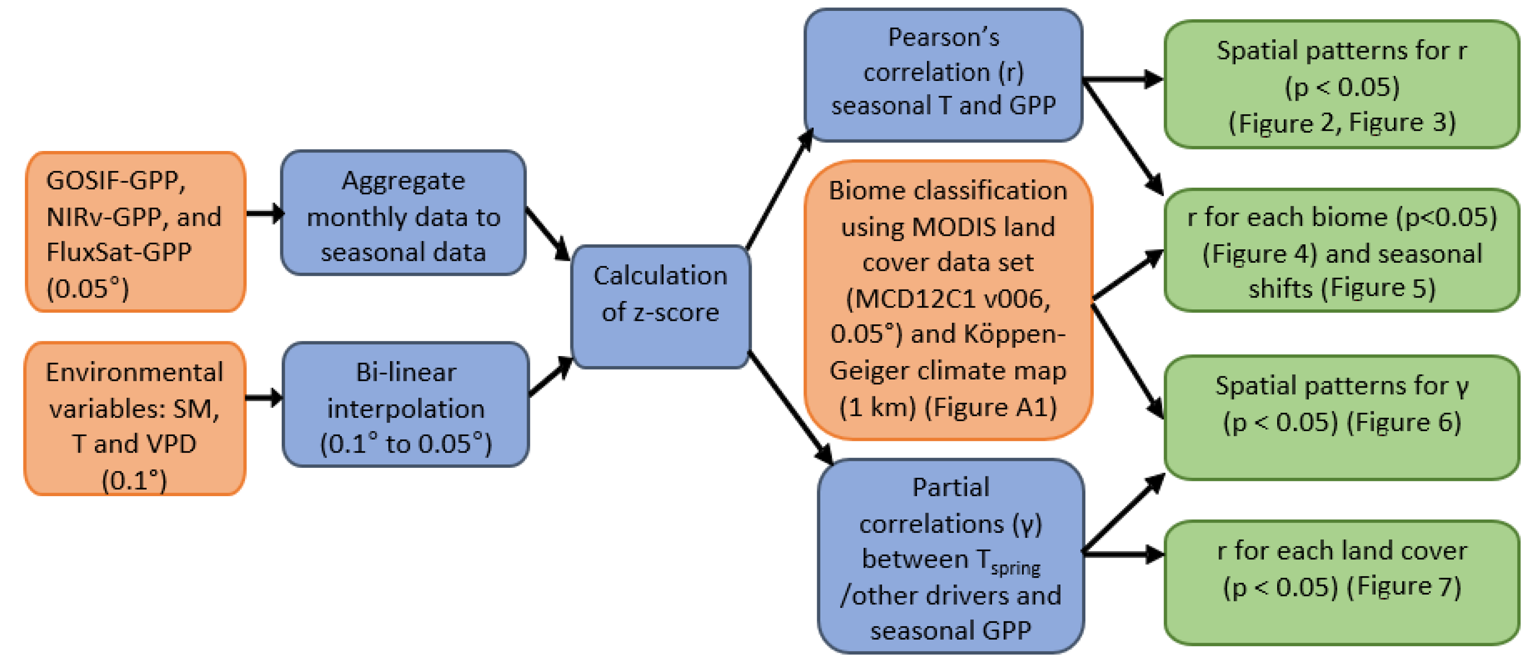
2.6. General Overview of Methodology
An overview of the workflow in this study is given in Figure 1, which illustrates the order of the main procedures. The methodology follows a similar scheme of comparable studies [5,6]. The data analysis was performed using Mathworks MATLAB, version 2020a.
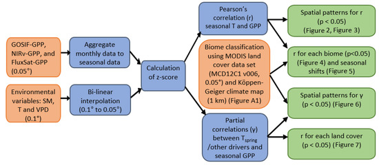
Figure 1.
The diagram of the study workflow. The input data (depicted in orange color) underwent pre-processing and statistics calculations (depicted in blue color), eventually leading to the main results (depicted in green color).
3. Results
3.1. Effects of Anomalies on Current and Post-Season GPP
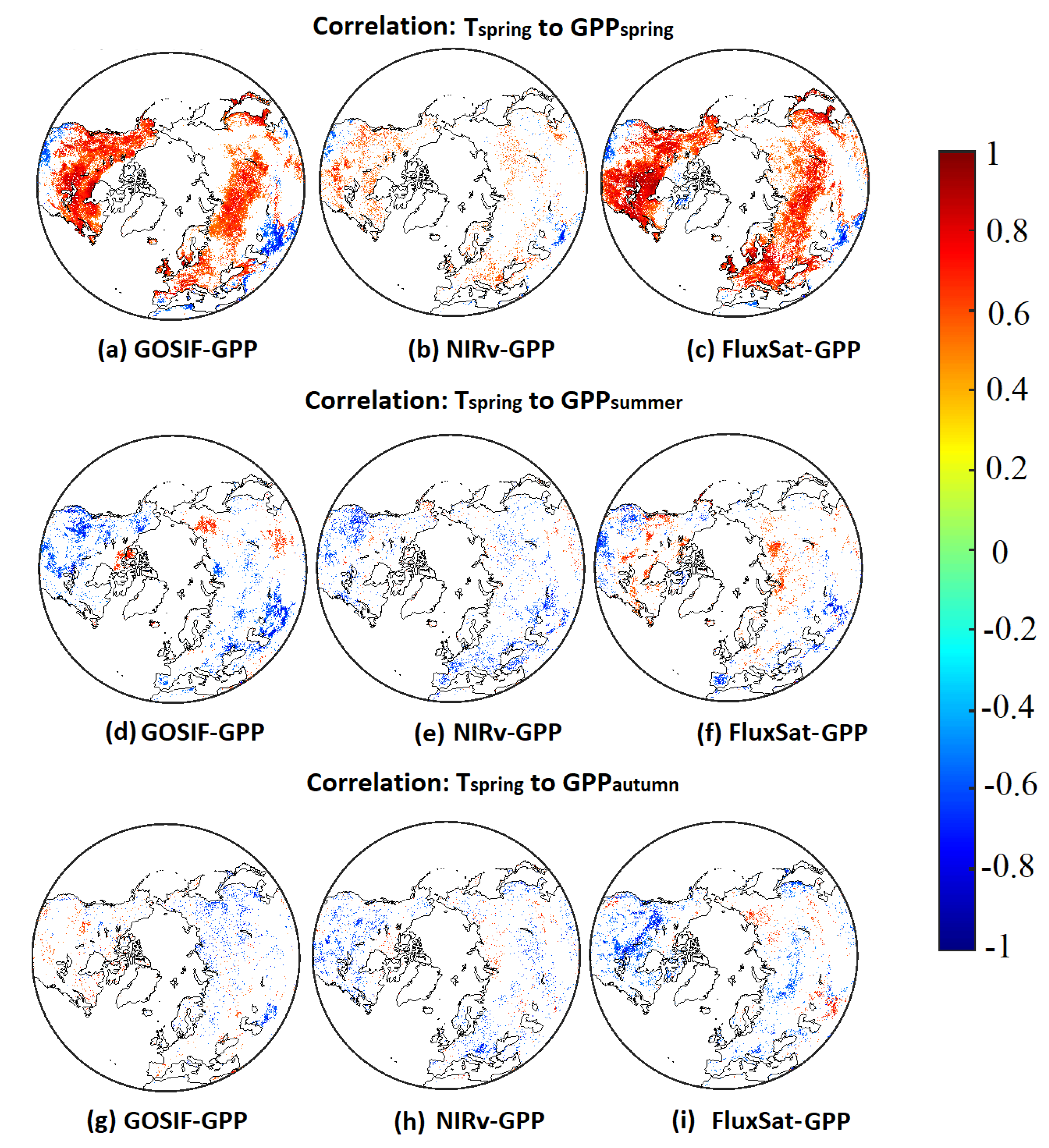
Pearson’s correlations between and showed similar spatial patterns in all three GPP products (Figure 2a–c). A high positive correlation dominated the mid- and high latitudes. Only the southwestern part of North America and South Asia showed a negative correlation. The same pattern was seen in all three products, however, NIRv-GPP had fewer significant correlations, resulting in a sparser pattern.
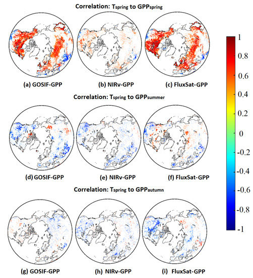
Figure 2.
Pearson’s correlations () between anomalies and (a–c)/ (d–f)/ (g–i).
Lagged effects of anomalies on showed fairly similar effects on certain land areas, and a larger difference among different GPP products was noticeable in the Arctic tundra and North Eurasia (Figure 2d–f). All three GPP products showed negative correlations in North America as well as Southeast Eurasia. The Arctic displayed clear positive effects in GOSIF-GPP and FluxSat-GPP, whereas negative effects dominated the response in NIRv-GPP.
Legacy effects from anomalies on were consistent to legacy effects from summer in the large southern areas (Figure 2g–i). However, GOSIF-GPP showed positive effects in North America, where negative effects were found in NIRv-GPP and FluxSat-GPP. Particularly, PW (Hudson Bay and West Siberia) showed strong negative effects in FluxSat-GPP. Some sporadic patches of positive correlations in Eurasia were also found in NIRv-GPP and FluxSat-GPP.
3.2. Latitudinal Distributions for Legacy Effects of Anomalies on and
Latitudinal distributions for legacy effects of anomalies on and were quantified based on their Pearson’s correlation coefficients (mean and one standard deviation) calculated across all the longitudes at each latitude interval of 0.05 (Figure 3). As the legacy effects largely oscillated in the high latitudes, the results were shown based on a moving average of every five pixels along the latitude. In general, all three GPP products showed positive legacy effects in most areas at north of and negative legacy effects in lower latitudes. GOSIF-GPP and NIRv-GPP had a fairly similar distribution of the legacy effects on , however, NIRv-GPP and FluxSat-GPP had a similar distribution of the legacy effects on . FluxSat-GPP differed from the other two in regards to , where positive legacy effects began to dominate further south, at ∼43N compared to >N for GOSIF-GPP and NIRv-GPP. FluxSat-GPP also displayed a strong negative peak at 55N–60N for , which almost has an inverse pattern of the legacy effects seen in summer.
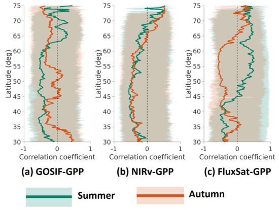
Figure 3.
Latitudinal distribution of Pearson’s correlations () between anomaly to summer (green) and autumn (orange) GPP anomaly, for: (a) GOSIF-GPP, (b) NIRv-GPP, and (c) FluxSat-GPP. The shaded area represents one standard deviation for the pixels with each latitude intervals (0.05). The solid line represents the mean values for the pixels with each latitude intervals. All the values have been processed using the moving average of every five consecutive latitudes.
3.3. Effects of Anomalies on GPP, GPP, and GPP for Each Biome
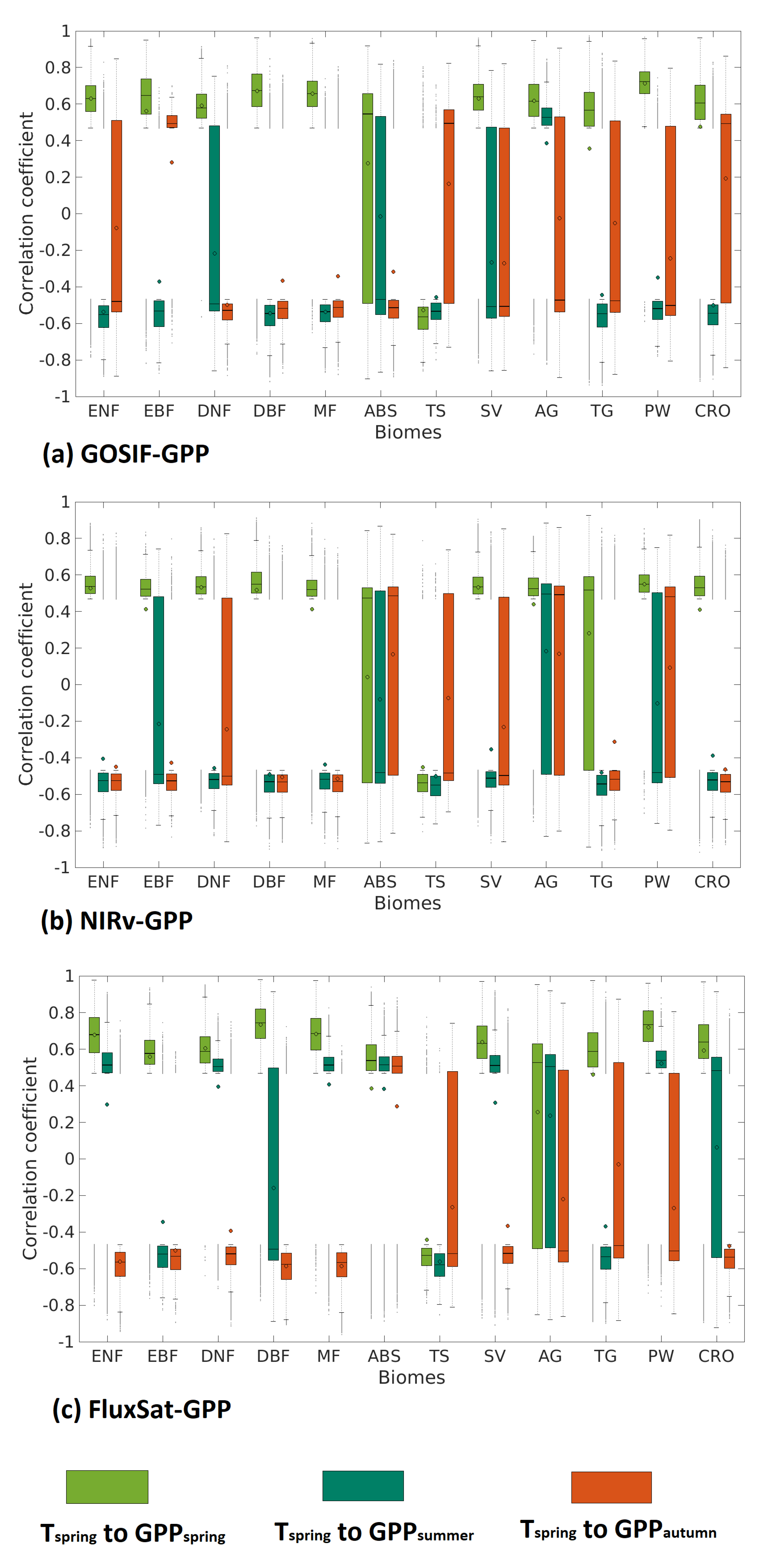
Effects of anomalies on , and GPP were aggregated for each biome based on all three GPP products (Figure 4). Results between GOSIF-GPP, NIRv-GPP and FluxSat-GPP were similar, but differed on certain biomes. In general, the forest biomes had a smaller statistical spread around negative correlations, meaning that these negative effects were specific to trees rather than herbaceous vegetation. The other biomes had a wider statistical spread, stretching across both positive and negative impacts, meaning that the overall impact is more neutral. FluxSat-GPP, on average, showed more positive correlations, particularly in summer. ABS and AG stood out from the rest with overall positive impacts, implying that drought propagation from increased is not promoted to the same extent here, as seen in biomes located further south.

Figure 4.
Boxplot of correlation coefficients to GPP, GPP, and GPP (spring: light green, summer: green and autumn: orange), for: (a) GOSIF-GPP, (b) NIRv-GPP, and (c) FluxSat-GPP. The mean value is represented by a small circle, and the median by a line.
3.4. Transition Patterns for Legacy Effects of on GPP and GPP
How legacy effects of propagated through summer and autumn was investigated based on spatial distribution of transition patterns and their aggregation for different biomes (Figure 5). Insignificant correlations are denoted by /, positive by +, and negative by −. The majority of legacy effects was found either in summer or autumn, meaning that the legacy effects only propagated one season. GOSIF-GPP and NIRv-GPP were dominated by a negative impact in summer (−/), whereas FluxSat-GPP revealed more pixels of a positive impact in summer (+/) and a negative impact in autumn (/−). This means that the timing of water-stress induced by the pre-season stimulated vegetation growth may vary between the GPP data sets.
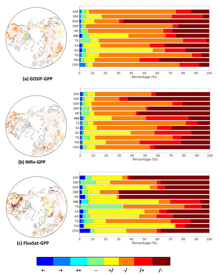
Figure 5.
Transition patterns of legacy effects from T anomalies on GPP and GPP for each biome, for: (a) GOSIF-GPP, (b) NIRv-GPP, and (c) FluxSat-GPP. The labels should be interpreted as follows: +− means there was a positive significant impact seen in summer and a negative in autumn, /− means there was an insignificant correlation seen in summer and a significant negative correlation in autumn). There were a total of eight different transition patterns excluding //, which means no significant legacy for both summer and autumn.
Separating the transition patterns based on biomes further reveals the similarity between GOSIF-GPP and NIRv-GPP, that is, the northern biomes (ABS and AG) showed a clear positive impact during summer. However, FluxSat-GPP showed positive impact in wetlands (PW), savannas (SV) and DNF during summer.
3.5. Dominant Drivers for GPP and GPP
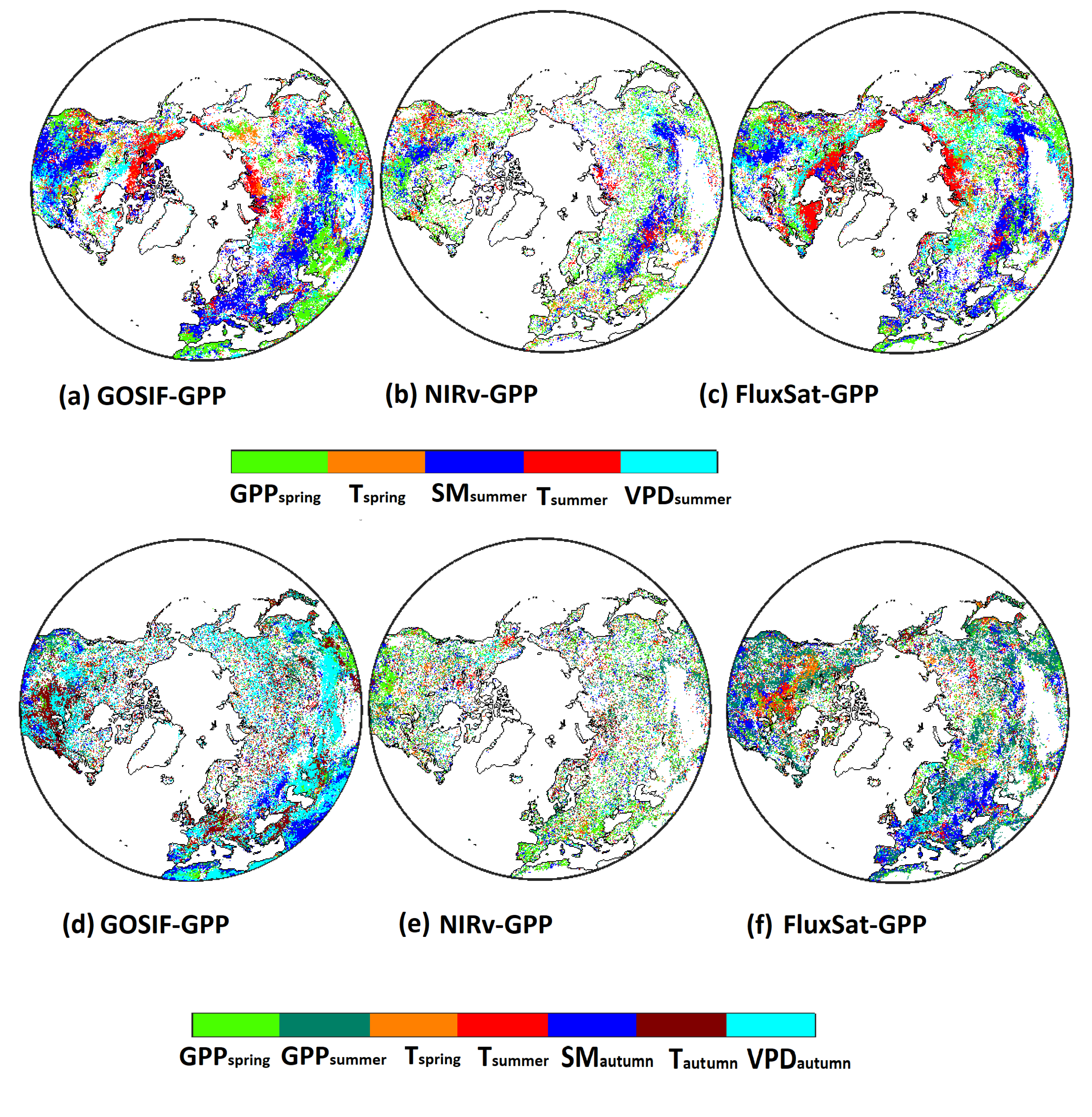
The dominant drivers for GPP showed similar spatial patterns in all three GPP products (Figure 6a–c). In summer, the arctic plant productivity was strongly correlated with temperature, whereas temperate regions showed soil moisture (SM) as the dominant driver. These temperature-dominant patterns also agreed with the patterns for positive legacy effects of T on GPP (Figure 3d–f). Legacy effects from GPP were the dominant driver in many regions, but legacy effects from T were not strong enough to surpass the importance of other drivers.
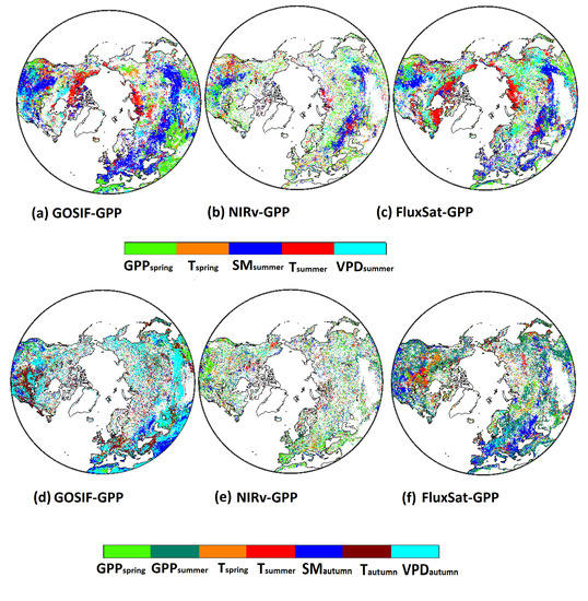
Figure 6.
Dominant variables that explain variance of GPP (a–c) and GPP (d–f) for the three GPP products (i.e., GOSIF-GPP, NIRv-GPP, and FluxSat-GPP). The dominant driver was identified based on the highest correlation coefficient (absolute value).
In contrast to summer, the dominant drivers of GPP were more diverse among the three GPP products (Figure 6d–f). GOSIF-GPP showed strong dependence on current seasonal drivers (e.g., T, VPD, and SM). For NIRv-GPP, the legacy effects were mostly dominated by GPP. For FluxSat-GPP, GPP, T, and SM were found to be the most important drivers.
3.6. The Importance of Drivers on GPP and GPP Aggregated on the Biome Level
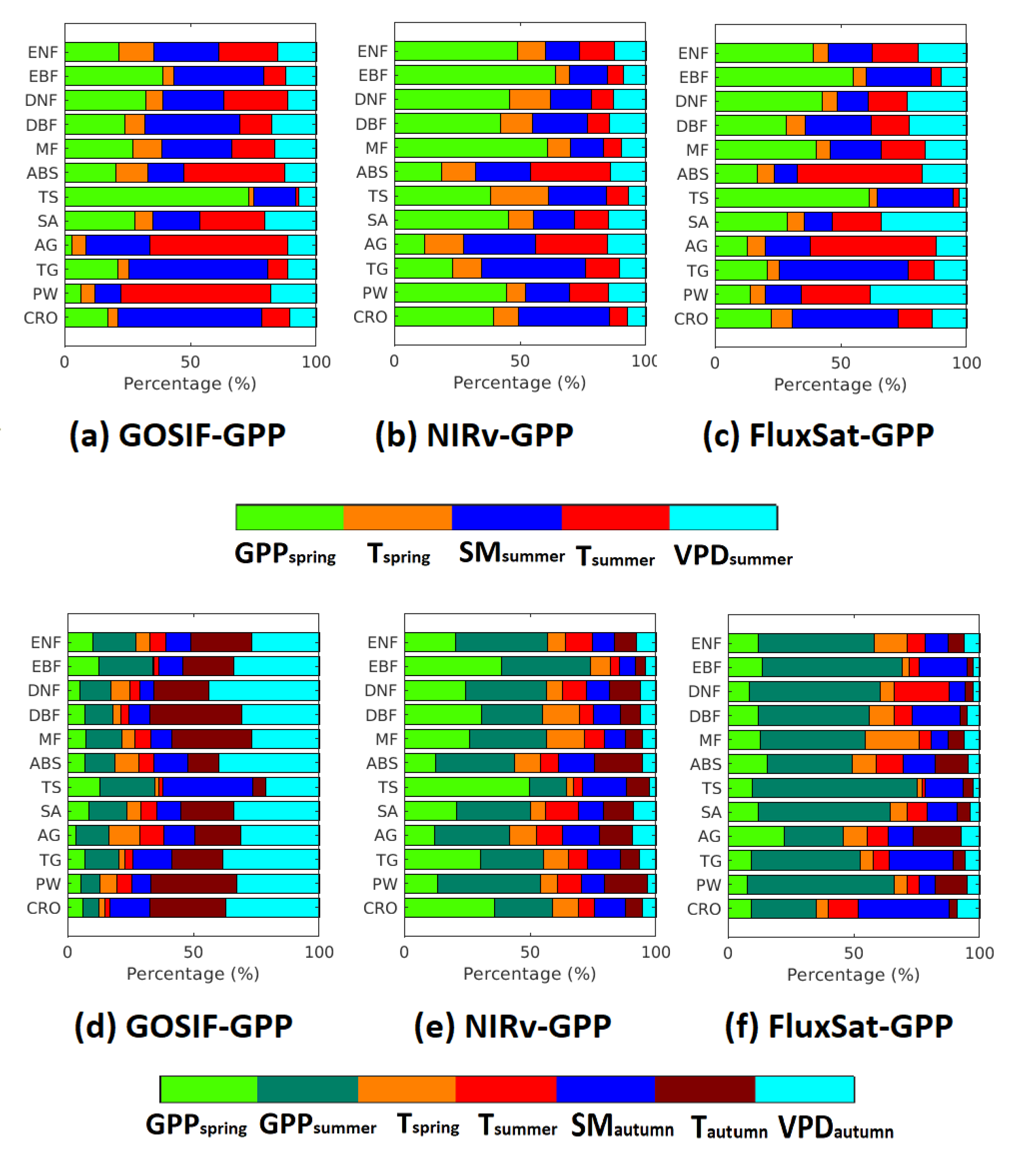
The important drivers for GPP and GPP were analyzed based on the biome level (Figure 7). Both environmental variables and biological variables (i.e., pre-season GPP) have been accounted for. Generally, the largest number of pixels that showed the significant correlation was found in FluxSat-GPP, followed by GOSIF-GPP and NIRv-GPP (Table 4). For the spatial patterns of the dominant driver, only the pixels with significant correlations were considered.
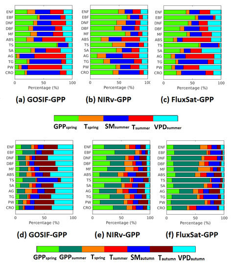
Figure 7.
Relative importance (%) of environmental and biological drivers on GPP (a–c) and GPP (d–f) based on different biomes.
Table 4.
Percentage of pixels with significant correlations, as seen in Figure 7 divided by biome-type and season. The first three columns correspond to summer, and the following to autumn.
The dominant driver varied depending on biome types, but overall, all three GPP data sets showed that among all the biomes, the smallest legacy effects from pre-season GPP were found in ABS and AG. These effects persisted in both summer and autumn. For these two biomes, temperature was the dominant driver for GPP. However, for the GPP, VPD was the dominant driver in GOSIF-GPP and GPP was the dominant driver in NIRv-GPP and FluxSat-GPP. Generally, the forest biomes showed larger legacy effects from pre-season GPP than other biomes in summer and autumn. For the current season drivers (i.e., soil moisture, temperature, and VPD), the contributions to GPP were larger than GPP. The contributions of these drivers were larger in GOSIF-GPP than in NIRv-GPP and FluxSat-GPP. Croplands showed the least amount of effects from the pre-season drivers.
4. Discussion
is reported to cause both negative and positive direct impacts on ecosystem productivity [6,16], but our results make a case for the latter being the dominant influence, at least in the mid- to high latitudes. Damage from, e.g., late spring frost events or acute frost desiccation does not seem to override the growth caused by warming, at least on a global scale. The only biome-type deviation from this trend is temperate shrublands, mainly located in north Africa and Turkey, in other words, close to the southernmost borders of our study area. These regions are known for their warm and dry climate. Warm springs in these regions likely bring adverse effects on water-stressed plants, causing a negative correlation.
The cohesive correlation trend between spring temperatures and spring productivity does not persist in the same vein for the legacy effects. A warm spring will not necessarily lead to the same legacy effects to summer and autumn productivity, as an unusually lush and productive spring would. The fact that these two usually go hand in hand makes this result somewhat surprising, but also highlights the importance of keeping these qualities separate. The legacy effects from warmer springs with high ecosystem productivity also differ strongly between GPP products. There are several uncertainties in the data sets that could contribute to this. One possible explanation, pointed out in [37], is the difficulty to separate snow cover decrease from leaf area increase. The spring months, particularly in the northernmost regions, are often characterized by partially covered snow. Increasing temperatures might lower the fraction of snow cover in spring, leading to a false signal of greening.
Our results also indicate that forests overall had the most prevalent negative responses from the legacy effects, whereas grasslands and shrublands showed an ambiguous response (Figure 4). The patterns (i.e., narrow spread of correlation coefficients in forests and wide spread of correlation coefficients in other types) are seen in all three GPP products. This result is much in line with previous studies (e.g., [16,17,18,19]). The authors of [16] used the Global Inventory Modeling and Mapping Studies (GIMMS) NDVI data set [38] and actual evapotranspiration derived from the FLUXNET latent heat flux measurements [39] to investigate the legacy effects of earlier springs on boreal forests in North America. They found that earlier spring and associated drying in summer can cause a decline of vegetation productivity due to increased tree mortality and fire activity. Possibly, the long seasonal time frames that the legacy effects operate on better match the slow growth seen in forests. In general, grasslands and shrublands are rapidly growing and changing across the seasons, and respond more directly to current-season precipitation and soil moisture conditions. The importance from previous seasons was then less evident. The legacy effects that were visible for grasslands and shrublands mostly occurred during summer. Moreover, the soil moisture data sets used in this study only reflected water contents of the topsoil horizon (0–7 cm), which may explain that grasslands or shrublands with the low rooting depth are more sensitive to the topsoil moisture condition than forests. This agrees with a study [40] which is based on eddy covariance measurements of carbon flux for Swiss forests and grasslands. They found that grasslands are more sensitive to spring drought because forests can reduce their evapotranspiration to increase the water use efficiency reflecting a better adaptive strategy.
Significant difference between GOSIF-GPP, NIRv-GPP, and FluxSat-GPP is a recurring theme for our results. Most likely, this is explained by fundamental differences in the models used to up-scale the data sets, as well as the measurement gaps that occur between different sensors. Satellite data sets of even higher spatial resolutions and quality might be necessary to bridge this gap and create a cohesive signal. On average, the least amount of significant correlations was seen using the NIRv-GPP product. Possibly, it has a weaker connection to surrounding climate variables than the other two products, as this data set relies more heavily on spectral radiation measurements. Further, outward disturbances on GPP, such as forest fires, anthropogenic land-cover change, or insect attacks, are not accounted for. Ideally, these factors should give rise to low significant correlations and thus be excluded from the analysis. However, the extent to which this has occurred is unclear. The modeling used to fill in the gaps for GOSIF-GPP and FluxSat-GPP could also, to some degree, explain the differences seen in dominating drivers between the three products. Climate variables such as soil moisture and temperature were generally considered more important for GOSIF-GPP and FluxSat-GPP, possibly an echo from utilizing climate variables as input to fill the gaps. Still, for the northern high latitudes, temperature increase has been shown to be the main factor facilitating increased plant productivity in summer [37,41]. However, our results also indicate a relatively cohesive north-south gradient trend of climate vegetation controls during summer, meaning ambiguity between different data-sets and types of vegetation indices can be bridged.
Further, the changes in the dominant climate drivers, particularly during the autumn season, could be the result of a relatively marginal difference between a cluster of controls, where the legacy effects from previous seasons also play an important part [42]. This ambiguity between controls of the late season is to some degree also reflected in previous research, e.g., work by [43] indicates that light limitation is also an important factor for autumn productivity in northern ecosystems. To include this driver in our analysis might therefore lead to a more cohesive result between products. In addition, [35,44] find that there is a complex coupling between soil moisture and temperature, both of which seem to be important controls towards the end of the growing season (a proxy for autumn productivity in this context). In an increasingly warmer world, the limitations imposed by temperature during autumn may shift to an expansion of mainly water-limited ecosystems, where the legacy effects from previous seasons may be amplified even further.
5. Conclusions
Propagating impacts from spring growth and temperature anomalies have been shown to affect summer and autumn ecosystem productivity in the Northern Hemisphere. These legacy effects are mostly negative and set in either in summer or autumn. The forest biomes (ENF, DBF, MF) show conclusive signals of negative impacts for all three GPP products in summer and autumn, whereas shrublands, croplands, and wetlands have a wider statistical spread between positive and negative impacts, leading to a more neutral overall impact. Only the northernmost biomes, AG and ABS, seem to conclusively show lagged positive impacts from spring temperature anomalies, which is important to account for in carbon-cycle models.
Results also seem to depend on the type of method used to quantify GPP, which somewhat may diminish the credibility of our findings. This mainly applies to the main drivers that affect browning and greening trends seen in the seasonal GPP. The effect on GPP from temperature change is most likely not linear and many factors are involved. Continuous development of higher-resolution GPP data sets is needed to further assess vegetation response to a warming climate.
Author Contributions
Conceptualization, W.Z. and H.M.; methodology, W.Z. and H.M.; software, H.M.; validation, W.Z. and H.M.; formal analysis, H.M.; investigation, H.M. and W.Z.; resources, W.Z.; data curation, W.Z.; writing—original draft preparation, H.M.; writing—review and editing, H.M. and W.Z.; visualization, H.M.; supervision, W.Z.; project administration, W.Z.; funding acquisition, W.Z. All authors have read and agreed to the published version of the manuscript.
Funding
This research was funded by a grant from the Swedish National Space Agency (209/19).
Data Availability Statement
The ERA5-land products can be downloaded via (https://cds.climate.copernicus.eu/cdsapp#!/dataset/reanalysis-era5-land?tab=overview). The GOSIF-GPP data sets can be downloaded via (https://globalecology.unh.edu/data/GOSIF-GPP.html). The NIRv-GPP data sets can be downloaded via (https://data.tpdc.ac.cn/en/data/d6dff40f-5dbd-4f2d-ac96-55827ab93cc5/). The FluxSat-GPP can be downloaded via (https://avdc.gsfc.nasa.gov/pub/tmp/FluxSat_GPP/, all accessed on 6 March 2022).
Acknowledgments
The author acknowledges the support by the Center for Scientific and Technical Computing at Lund University for data storage and computation via the project (SNIC 2021/6-341 and LU 2021/2-115).
Conflicts of Interest
The authors declare no conflict of interest.
Abbreviations
The following abbreviations are used in this manuscript:
| ABS | Arctic and Boreal Shrublands |
| AG | Arctic Grasslands |
| AVHRR | Advanced Very High Resolution Radiometer |
| BRDF | Bidirectional Reflectance Distribution Function |
| CRO | Croplands |
| DBF | Deciduous Broadleaf Forests |
| DNF | Deciduous Needleleaf Forests |
| EBF | Evergreen Broadleaf Forests |
| EC | Eddy Co-variance |
| ECMWF | European Centre for Medium-Range Weather Forecasts |
| ENF | Evergreen Needleleaf Forests |
| EVI | Enhanced Vegetation Index |
| FluxSat | Fluxnet Data Fused with Satellite Images |
| GOME | Global Ozone Monitoring Experiment |
| GOSIF | the Global, OCO-2-based SIF Product |
| GPP | Gross Primary Productivity |
| IGBP | International Geosphere-Biosphere Programme |
| LTDR | Land Long-Term Data Record |
| MF | Mixed Forests |
| MODIS | Moderate Resolution Imaging Spectrometer |
| NDVI | Normalized Difference Vegetation Index |
| NIRv | Near-infrared Reflectance of Vegetation |
| OCO-2 | Orbiting Carbon Observatory-2 |
| PAR | Photosynthetic Active Radiation |
| PW | Permanent Wetlands |
| SIF | Solar Induced Fluorescence |
| SM | Soil Moisture |
| SV | Savannas |
| T | Temperature |
| TG | Temperate Grasslands |
| TS | Temperate Shrublands |
| VPD | Vapor Pressure Deficit |
Appendix A

Figure A1.
In total, 12 biomes comprise the study area—Evergreen Needleleaf Forests (ENF), Evergreen Broadleaf Forests (EBF), Deciduous Needleleaf Forests (DNF), Decidous Broadleaf Forests (DBF), Mixed forests (MF), Arctic and Boreal Shrublands (ABS), Temperate Shrublands (TS), Savannas (SV), Arctic Grasslands (AG), Temperate Grasslands (TG), Permanent Wetlands (PW), and Croplands (CRO).
References
- IPCC. Climate Change 2014: Synthesis Report. Contribution of Working Groups I, II and III to the Fifth Assessment Report of the Intergovernmental Panel on Climate Change; Pachauri, R.K., Meyer, L.A., Eds.; Core Writing Team: Geneva, Switzerland, 2014. [Google Scholar]
- Piao, S.; Liu, Q.; Chen, A.; Janssens, I.A.; Fu, Y.; Dai, J.; Liu, L.; Lian, X.; Shen, M.; Zhu, X. Plant phenology and global climate change: Current progresses and challenges. Glob. Chang. Biol. 2019, 25, 1922–1940. [Google Scholar] [CrossRef] [PubMed]
- Lian, X.; Piao, S.; Chen, A.; Wang, K.; Li, X.; Buermann, W.; Huntingford, C.; Peñuelas, J.; Xu, H.; Myneni, R.B. Seasonal biological carryover dominates northern vegetation growth. Nat. Commun. 2021, 12, 983. [Google Scholar] [CrossRef] [PubMed]
- Zhang, W.; Döscher, R.; Koenigk, T.; Miller, P.; Jansson, C.; Samuelsson, P.; Wu, M.; Smith, B. The interplay of recent vegetation and sea ice dynamics—results from a regional Earth system model over the Arctic. Geophys. Res. Lett. 2020, 47, e2019GL085982. [Google Scholar] [CrossRef]
- Buermann, W.; Forkel, M.; O’sullivan, M.; Sitch, S.; Friedlingstein, P.; Haverd, V.; Jain, A.K.; Kato, E.; Kautz, M.; Lienert, S.; et al. Widespread seasonal compensation effects of spring warming on northern plant productivity. Nature 2018, 562, 110–114. [Google Scholar] [CrossRef] [Green Version]
- Bastos, A.; Ciais, P.; Friedlingstein, P.; Sitch, S.; Pongratz, J.; Fan, L.; Wigneron, J.; Weber, U.; Reichstein, M.; Fu, Z.; et al. Direct and seasonal legacy effects of the 2018 heat wave and drought on European ecosystem productivity. Sci. Adv. 2020, 6, eaba2724. [Google Scholar] [CrossRef] [PubMed]
- Piao, S.; Tan, J.; Chen, A.; Fu, Y.H.; Ciais, P.; Liu, Q.; Janssens, I.A.; Vicca, S.; Zeng, Z.; Jeong, S.J.; et al. Leaf onset in the northern hemisphere triggered by daytime temperature. Nat. Commun. 2015, 6, 6911. [Google Scholar] [CrossRef] [PubMed] [Green Version]
- Jin, H.; Jönsson, A.M.; Olsson, C.; Lindström, J.; Jönsson, P.; Eklundh, L.; Yohe, G. New satellite-based estimates show significant trends in spring phenology and complex sensitivities to temperature and precipitation at northern European latitudes. Int. J. Biometeorol. 2019, 63, 763–775. [Google Scholar] [CrossRef] [PubMed] [Green Version]
- Weijers, S.; Myers-Smith, I.; Löffler, J. A warmer and greener cold world: Summer warming increases shrub growth in the alpine and high arctic tundra. Erdkunde 2018, 72, 63–85. [Google Scholar] [CrossRef] [Green Version]
- Berner, L.T.; Massey, R.; Jantz, P.; Forbes, B.C.; Macias-Fauria, M.; Myers-Smith, I.; Kumpula, T.; Gauthier, G.; Andreu-Hayles, L.; Gaglioti, B.V.; et al. Summer warming explains widespread but not uniform greening in the Arctic tundra biome. Nat. Commun. 2020, 11, 4621. [Google Scholar] [CrossRef]
- Kunert, N.; Hajek, P.; Hietz, P.; Morris, H.; Rosner, S.; Tholen, D. Summer temperatures reach the thermal tolerance threshold of photosynthetic decline in temperate conifers. Plant Biol. 2021. [Google Scholar] [CrossRef] [PubMed]
- Piao, S.; Ciais, P.; Friedlingstein, P.; Peylin, P.; Reichstein, M.; Luyssaert, S.; Margolis, H.; Fang, J.; Barr, A.; Chen, A.; et al. Net carbon dioxide losses of northern ecosystems in response to autumn warming. Nature 2008, 451, 49–52. [Google Scholar] [CrossRef] [PubMed]
- Pongratz, J.; Reick, C.H.; Raddatz, T.; Claussen, M. Biogeophysical versus biogeochemical climate response to historical anthropogenic land cover change. Geophys. Res. Lett. 2010, 37, L08702. [Google Scholar] [CrossRef] [Green Version]
- Zhang, Y.; Song, C.; Band, L.E.; Sun, G.; Li, J. Reanalysis of global terrestrial vegetation trends from MODIS products: Browning or greening? Remote Sens. Environ. 2017, 191, 145–155. [Google Scholar] [CrossRef] [Green Version]
- Lian, X.; Piao, S.; Li, L.Z.; Li, Y.; Huntingford, C.; Ciais, P.; Cescatti, A.; Janssens, I.A.; Peñuelas, J.; Buermann, W.; et al. Summer soil drying exacerbated by earlier spring greening of northern vegetation. Sci. Adv. 2020, 6, eaax0255. [Google Scholar] [CrossRef] [PubMed] [Green Version]
- Buermann, W.; Bikash, P.R.; Jung, M.; Burn, D.H.; Reichstein, M. Earlier springs decrease peak summer productivity in North American boreal forests. Environ. Res. Lett. 2013, 8, 024027. [Google Scholar] [CrossRef]
- Parida, B.R.; Buermann, W. Increasing summer drying in North American ecosystems in response to longer nonfrozen periods. Geophys. Res. Lett. 2014, 41, 5476–5483. [Google Scholar] [CrossRef]
- Kelsey, K.C.; Pedersen, S.H.; Leffler, A.J.; Sexton, J.O.; Feng, M.; Welker, J.M. Winter snow and spring temperature have differential effects on vegetation phenology and productivity across Arctic plant communities. Glob. Chang. Biol. 2021, 27, 1572–1586. [Google Scholar] [CrossRef]
- Wipf, S.; Rixen, C. A review of snow manipulation experiments in Arctic and alpine tundra ecosystems. Polar Res. 2010, 29, 95–109. [Google Scholar] [CrossRef]
- Camps-Valls, G.; Campos-Taberner, M.; Moreno-Martínez, Á.; Walther, S.; Duveiller, G.; Cescatti, A.; Mahecha, M.D.; Muñoz-Marí, J.; García-Haro, F.J.; Guanter, L.; et al. A unified vegetation index for quantifying the terrestrial biosphere. Sci. Adv. 2021, 7, eabc7447. [Google Scholar] [CrossRef] [PubMed]
- Wu, X.; Guo, W.; Liu, H.; Li, X.; Peng, C.; Allen, C.D.; Zhang, C.; Wang, P.; Pei, T.; Ma, Y.; et al. Exposures to temperature beyond threshold disproportionately reduce vegetation growth in the northern hemisphere. Natl. Sci. Rev. 2018, 6, 786–795. [Google Scholar] [CrossRef]
- Li, X.; Xiao, J. A Global, 0.05-Degree Product of Solar-Induced Chlorophyll Fluorescence Derived from OCO-2, MODIS, and Reanalysis Data. Remote Sens. 2019, 11, 517. [Google Scholar] [CrossRef] [Green Version]
- Badgley, G.; Field, C.B.; Berry, J.A. Canopy near-infrared reflectance and terrestrial photosynthesis. Sci. Adv. 2017, 3, e1602244. [Google Scholar] [CrossRef] [PubMed] [Green Version]
- Wang, S.; Zhang, Y.; Ju, W.; Qiu, B.; Zhang, Z. Tracking the seasonal and inter-annual variations of global gross primary production during last four decades using satellite near-infrared reflectance data. Sci. Total Environ. 2021, 755, 142569. [Google Scholar] [CrossRef] [PubMed]
- Joiner, J.; Yoshida, Y.; Zhang, Y.; Duveiller, G.; Jung, M.; Lyapustin, A.; Wang, Y.; Tucker, C.J. Estimation of terrestrial global gross primary production (GPP) with satellite data-driven models and eddy covariance flux data. Remote Sens. 2018, 10, 1346. [Google Scholar] [CrossRef] [Green Version]
- Friedl, M.; Sulla-Menashe, D. MCD12C1 MODIS/Terra+Aqua Land Cover Type Yearly L3 Global 0.05Deg CMG V006; NASA EOSDIS Land Processes DAAC: Sioux Falls, SD, USA, 2015. [Google Scholar] [CrossRef]
- Kottek, M.; Grieser, J.; Beck, C.; Rudolf, B.; Rubel, F. World Map of the Köppen-Geiger Climate Classification Updated. Meteorol. Zeitschrif 2006, 15, 259–263. [Google Scholar] [CrossRef]
- Peel, M.C.; Finlayson, B.L.; McMahon, T.A. Updated world map of the Köppen-Geiger climate classification. Hydrol. Earth Syst. Sci. 2007, 11, 1633–1644. [Google Scholar] [CrossRef] [Green Version]
- Belward, A.S. The IGBP-DIS global 1-km land-cover data set DIS-Cover: A project overview. Photogramm. Eng. Remote Sens. 1999, 65, 1013–1020. [Google Scholar]
- Li, X.; Xiao, J. Mapping photosynthesis solely from solar-induced chlorophyll fluorescence: A global, fine-resolution dataset of gross primary production derived from OCO-2. Remote Sens. 2019, 11, 2563. [Google Scholar] [CrossRef] [Green Version]
- Li, J.; Tam, C.Y.; Tai, A.P.; Lau, N.C. Vegetation-heatwave correlations and contrasting energy exchange responses of different vegetation types to summer heatwaves in the Northern Hemisphere during the 1982–2011 period. Agric. For. Meteorol. 2021, 296, 108208. [Google Scholar] [CrossRef]
- Friedl, M.A.; Gray, J.M.; Melaas, E.K.; Richardson, A.D.; Hufkens, K.; Keenan, T.F.; Bailey, A.; O’Keefe, J. A tale of two springs: Using recent climate anomalies to characterize the sensitivity of temperate forest phenology to climate change. Environ. Res. Lett. 2014, 9, 054006. [Google Scholar] [CrossRef]
- Muñoz-Sabater, J.; Dutra, E.; Agustí-Panareda, A.; Albergel, C.; Arduini, G.; Balsamo, G.; Boussetta, S.; Choulga, M.; Harrigan, S.; Hersbach, H.; et al. ERA5-Land: A state-of-the-art global reanalysis dataset for land applications. Earth Syst. Sci. Data 2021, 13, 4349–4383. [Google Scholar] [CrossRef]
- Yuan, W.; Zheng, Y.; Piao, S.; Ciais, P.; Lombardozzi, D.; Wang, Y.; Ryu, Y.; Chen, G.; Dong, W.; Hu, Z.; et al. Increased atmospheric vapor pressure deficit reduces global vegetation growth. Sci. Adv. 2019, 5, eaax1396. [Google Scholar] [CrossRef] [Green Version]
- Liu, Q.; Fu, Y.H.; Zeng, Z.; Huang, M.; Li, X.; Piao, S. Temperature, precipitation, and insolation effects on autumn vegetation phenology in temperate China. Glob. Chang. Biol. 2016, 22, 644–655. [Google Scholar] [CrossRef] [PubMed]
- Zhou, S.; Zhang, Y.; Ciais, P.; Xiao, X.; Luo, Y.; Caylor, K.; Huang, Y.; Wang, S. Dominant role of plant physiology in trend and variability of gross primary productivity in North America. Sci. Rep. 2017, 7, 41366. [Google Scholar] [CrossRef] [PubMed] [Green Version]
- Piao, S.; Wang, X.; Park, T.; Chen, C.; Lian, X.; He, Y.; Bjerke, J.W.; Chen, A.; Ciais, P.; Tømmervik, H.; et al. Characteristics, drivers and feedbacks of global greening. Nat. Rev. Earth Environ. 2020, 1, 14–27. [Google Scholar] [CrossRef]
- Tucker, C.J.; Pinzon, J.E.; Brown, M.E.; Slayback, D.A.; Pak, E.W.; Mahoney, R.; Vermote, E.F.; Saleous, N.E. An extended AVHRR 8-km NDVI dataset compatible with MODIS and SPOT vegetation NDVI data. Int. J. Remote Sens. 2005, 26, 4485–4498. [Google Scholar] [CrossRef]
- Jung, M.; Reichstein, M.; Margolis, H.A.; Cescatti, A.; Richardson, A.D.; Arain, M.A.; Arneth, A.; Bernhofer, C.; Bonal, D.; Chen, J.; et al. Global patterns of land-atmosphere fluxes of carbon dioxide, latent heat, and sensible heat derived from eddy covariance, satellite, and meteorological observations. J. Geophys. Res. Biogeosciences 2011, 116, G00J07. [Google Scholar] [CrossRef] [Green Version]
- Wolf, S.; Eugster, W.; Ammann, C.; Häni, M.; Zielis, S.; Hiller, R.; Stieger, J.; Imer, D.; Merbold, L.; Buchmann, N. Contrasting response of grassland versus forest carbon and water fluxes to spring drought in Switzerland. Environ. Res. Lett. 2013, 8, 035007. [Google Scholar] [CrossRef] [Green Version]
- Xu, L.; Myneni, R.; Chapin Iii, F.; Callaghan, T.V.; Pinzon, J.; Tucker, C.J.; Zhu, Z.; Bi, J.; Ciais, P.; Tømmervik, H.; et al. Temperature and vegetation seasonality diminishment over northern lands. Nat. Clim. Chang. 2013, 3, 581–586. [Google Scholar] [CrossRef] [Green Version]
- Liu, Q.; Fu, Y.H.; Zhu, Z.; Liu, Y.; Liu, Z.; Huang, M.; Janssens, I.A.; Piao, S. Delayed autumn phenology in the Northern Hemisphere is related to change in both climate and spring phenology. Glob. Chang. Biol. 2016, 22, 3702–3711. [Google Scholar] [CrossRef] [PubMed]
- Zhang, Y.; Commane, R.; Zhou, S.; Williams, A.P.; Gentine, P. Light limitation regulates the response of autumn terrestrial carbon uptake to warming. Nat. Clim. Chang. 2020, 10, 739–743. [Google Scholar] [CrossRef]
- Zhang, Y.; Parazoo, N.C.; Williams, A.P.; Zhou, S.; Gentine, P. Large and projected strengthening moisture limitation on end-of-season photosynthesis. Proc. Natl. Acad. Sci. USA 2020, 117, 9216–9222. [Google Scholar] [CrossRef] [PubMed]


Publisher’s Note: MDPI stays neutral with regard to jurisdictional claims in published maps and institutional affiliations. |
© 2022 by the authors. Licensee MDPI, Basel, Switzerland. This article is an open access article distributed under the terms and conditions of the Creative Commons Attribution (CC BY) license (https://creativecommons.org/licenses/by/4.0/).