Rapid Tsunami Potential Assessment Using GNSS Ionospheric Disturbance: Implications from Three Megathrusts

Abstract

The current tsunami early warning systems always issue alarms once large undersea earthquakes are detected, inevitably resulting in false warnings since there are no deterministic scaling relations between earthquake size and tsunami potential. In this paper, we assess tsunami potential by analyzing co-seismic ionospheric disturbances (CIDs). We examined CIDs of three megathrusts (the 2014 M_w 8.2 Iquique, the 2015 M_w 8.3 Illapel, and the recent 2021 M_w 8.2 Alaska events) as detected by Global Navigation Satellite System (GNSS) observations. We found that CIDs near the epicenter generated by the 2021 M_w 8.2 Alaska event were significantly weaker than those of the two Chilean events, despite having similar earthquake magnitudes. The propagation direction of CIDs from the M_w 8.2 Alaska earthquake further revealed ruptures toward the deeper seismogenic zone, implying less seafloor uplift and hazardous flooding. Our work sheds light on incorporating GNSS-based CIDs for more trustworthy tsunami warning systems.

1. Introduction

Tsunami hazards and the necessity of reliable tsunami early warning systems have been drawing persistent research attention after the deadly 2004 M_w 9.0 Sumatra and 2011 M_w 9.1 Tohoku events [1,2,3]. In this regard, rapid earthquake source (magnitude, focal mechanism, and finite slip distribution) characterization approaches based on seismic or GNSS (Global Navigation Satellite System) or joint networks have been put forward in recent years [4,5,6]. However, these land-based networks only provide one-sided data, and thus the detailed rupture information cannot be fully determined, which may cause significant uncertainties for tsunami potential estimation and thus false alarms. For example, according to the 2006 U.S. Government Accountability Office report [7], in the Pacific Ocean, the false alarm rate was as high as 75%. False alarms produce significant negative economic and societal impacts, which undermine the credibility of the existing system and government agencies. Reducing the uncertainty level of tsunami early warning systems is of significance for early decision-making.

In addition to ground shaking and floods, submarine megathrusts also cause co-seismic ionospheric disturbances (CIDs) through lithosphere–atmosphere–ionospheric coupling [8,9,10], which can be retrieved by combing different frequencies of GNSS signals and easily distinguishing them from the normal traveling ionospheric disturbances (TIDs), based on scales and frequencies [11,12]. CIDs mainly originate from acoustic gravity waves by permanent seafloor deformation around the epicenter (AGW_epi) and propagating Rayleigh waves (AW_Rayleigh), and internal gravity waves by tsunamis (IGW_tsuna) that propagate upwards in an oblique direction. These different components of CIDs are usually distinguishable in terms of apparent velocity and frequency, and using GNSS ionospheric sounding could help characterize earthquake sources and identify tsunami potential. For example, despite having the same magnitude of M_w 7.8, the 2010 Mentawai earthquake generated much stronger CIDs than the Banyak earthquake [13,14], implying a significant vertical uplift, and the devastating tsunami can be identified as early as 8 min after the earthquake origin time. Complementary to conventional approaches, Manta et al. [13] concluded that GNSS ionospheric sounding provides valuable additional information to reduce the source uncertainness and improve the reliability of tsunami early warning systems.

However, the occurrence of a “tsunami earthquake” is comparably rare. To date, the 2010 M_w 7.8 Mentawai earthquake is the only well-instrumented “tsunami earthquake” that has ruptured the mostly shallow part of the subduction zone, and it remains unclear whether the conclusions by Manta et al. [13] could be projected to other events, especially for larger magnitudes but without damaging tsunami waves. Herein, we thus extended the scope to more frequent regular megathrusts that rupture both the deep and shallow parts of the subduction zone. Particularly, we selected three great M_w > 8 megathrusts: the 2014 M_w 8.2 Chile Iquique, the 2015 M_w 8.3 Chile Illapel, and the 2021 M_w 8.2 Alaska earthquakes. The Chilean events generated damaging tsunamis, while the Alaska earthquake produced negligible waves. We first extracted the CIDs caused by the three events and then performed an analysis on the CIDs’ propagation velocity, direction, and arrival time from spectra. We focused on the potential of identifying destructive and non-destructive tsunamis through the CIDs.

2. Materials and Methods

Figure 1 shows the epicenter, origin time, and focal mechanism solution of the three great M_w > 8 megathrusts (the 2014 M_w 8.2 Chile Iquique, the 2015 M_w 8.3 Chile Illapel, and the 2021 M_w 8.2 Alaska earthquakes) involved in this study.

In this paper, raw 30 s sampling GNSS measurements on the day of the earthquake archived at UNAVCO (ftp://data-out.unavco.org/pub/ accessed on 21 August 2021) were used to retrieve CIDs for the three megathrusts. We selected 33, 36, and 39 GNSS sites (see Figure 2a,b) providing ideal CID coverage for the 2014 M_w 8.2 Iquique, 2015 M_w 8.3 Illapel, and 2021 M_w Alaska events, respectively. The basic information of the 108 permanent dual-frequency stations selected is provided in Tables S1–S3. GNSS technology, with its high precision and continuity, has become one of the most important means of ionospheric modeling and monitoring [15]. We first utilized the widely adopted (see [16,17]) linear combination of the dual-frequency phase observations to estimate total electron content (TEC) or slant TEC (STEC) along the propagation path:

$$STEC=\frac{f_1^2{f}_2^2}{40.3\left(f_1^2-f_2^2\right)}\left[L_1-L_2+\left({\lambda }_1{N}_1-{\lambda }_2{N}_2\right)+b_r+b^s+\epsilon \right]$$

(1)

where f₁ and f₂ are signals transmitting frequencies; N₁ and N₂ are the integer ambiguities of L₁ and L₂, respectively; λ₁ and λ₂ are the wavelengths of the carrier; b_r and b^s are the differential code biases for the receiver and satellite, respectively; and ε is the observation noise.

Since the electron density distribution changes with altitude, here we assume a single-layer at 350 km (reaching the height of hmF2) [18,19,20]; we further obtained vertical TEC (VTEC) by mapping STEC with >20° elevation angles to the vertical:

$$VTEC=STEC\ast \cos \left[{\sin }^{-1}\left(\frac{R_r}{R_e+H}\sin \left(z\right)\right)\right]$$

(2)

where R_e is the radius of the Earth, R_r is the distance from the Earth center to the receiver, H is the height of the thin shell (H = 350 km), and z is the zenith angle. Through the time differences of geometry-free combinations of GNSS phase measurements [21], the accuracy of the TEC change estimation of approximately 0.01~0.02 TECU (TEC unit, 1 TECU = 10¹⁶ el/m²) can be expected [22,23].

By combining the ionospheric pierce point (IPP) position and the TEC variation during the period of interest, one can obtain the spatial distribution and dynamic characteristics of ionospheric disturbances. Note that IPP refers to the intersection of the signal path of the satellite-receiver pair and the thin-shell ionosphere; its projection on the ground is termed as sub-ionospheric points (SIPs). The satellite zenith angle at IPP is shown in Equation (3),

$$z^{\prime }={\sin }^{-1}\left(\frac{\sin \alpha \sin A}{\cos B_{IPP}}\right)$$

(3)

$$\alpha =z-z^{\prime }$$

(4)

the longitude and latitude of IPP are determined by:

$$B_{IPP}={\sin }^{-1}\left(\sin B_0\cos \alpha +\cos B_0\sin \alpha \cos A\right)$$

(5)

$$L_{IPP}=L_0+{\sin }^{-1}\left(\frac{\sin \alpha \sin A}{\cos B_{IPP}}\right)$$

(6)

where A is the azimuth of the satellite relative to the station, B₀ and L₀ are the latitude and longitude of the station, and α is the geocentric angle between the GNSS station and the IPP.

After obtaining the TEC series, we used bandpass filtering to remove the long-term variations and TEC background trend induced by ionospheric diurnal variabilities, IPP motion, and constant instrumental biases [24,25,26]. Here, we set the window length as 1–8 mHz for multiple coupled perturbations covering signals related to atmospheric gravity modes and acoustic modes [9,27]. In general, the fourth-order Butterworth bandpass filter is used to process the raw TEC sequences on account of its ideally flat magnitude [17,28]. Using the differential TEC (dTEC) sequence, ionospheric anomalies related to the rupture of the epicenter can be detected during a submarine earthquake.

3. Results

The tsunami triggered by the 2014 Iquique earthquake (M_w 8.2) produced some damage to the coastal area of Tarapaca in northern Chile (17° S–23° S) [29]. This tsunami was recorded around Pisagua and some ports located south of Iquique, and the Pacific Tsunami Warning Center (PTWC) issued an alert for this event. The first wave of the tsunami was recorded by the tide gauge PISA (70.21° W, 19.6° S) located west of the epicenter (~2 m), after which the tsunami wave height was reduced [30]. As for the 2015 M_w 8.3 Illapel earthquake, there was a significant tsunami impact on the coastal area between 26° S and 35° S. PTWC and the National Ocean Service (NOS) released tsunami threat information promptly, and the local government implemented evacuation work on the coast of Chile. The coast near the epicenter was quickly invaded by floods, and the tide gauge COQU (71.34° W, 29.95° S) north of the epicenter recorded the tsunami wave height as over 4 m. An asymmetric change of tsunami wave height was captured north and south of the epicenter [31]. On the contrary, despite all three events having the same magnitude and issuing warnings, the 29 July 2021 Alaska earthquake (M_w 8.2) did not produce a substantial tsunami impact in the vicinity of the epicenter. The tidal station SDPT (160.5017° W, 55.337° N) closest to the source recorded the tiny tsunami fluctuations (less than 0.25 m), and the wave height largely diminished in other stations.

The ionosphere over the epicentral area was perturbed to varying degrees by seafloor uplift and tsunami during all three events. During the period of interest in this study (within 2 h after the mainshock), there existed sufficient satellites over all three regions, and thus we could obtain dense arcs of IPP observations to extract disturbance time series. Specifically, there were seven satellites (PRN01, PRN11, PRN13, PRN17, PRN20, PRN23, and PRN32) over Iquique, six satellites (PRN02, PRN12, PRN14, PRN24, PRN25, and PRN29) over Illapel, and seven satellites (PRN02, PRN04, PRN07, PRN09, PRN16, PRN20, and PRN30) over Alaska, and trajectories of IPPs of the three earthquakes are shown in Figure 3a–c.

From the disturbances extracted by each satellite-station pair during the three earthquakes, the well-defined “N-type” ionospheric response was observed (e.g., each red series in Figure 4a–c), indicating that the ionospheric oscillation at this moment is related to the compression-rarefaction wave. Specifically, in the 2014 M_w 8.2 Iquique event, there were similar responses in the north and south of the source (Figure 4a), and satellite PRN01 showed the most significant fluctuations. During the earthquake, its IPPs were all located near the epicenter and moved from southwest to northeast. In the 2015 M_w 8.3 Illapel earthquake, only the north of the epicenter had clear TEC variations. Figure 4b shows the sequence of PRN25; during the earthquake, the IPPs moved closer to the epicenter and covered most of the north and south areas of the near field. As for the 2021 M_w 8.2 Alaska event, there was only a slight perturbation in a small area around the near field (Figure 4c); PRN04 is a clear case with good geometric observation conditions. The results of the ionospheric perturbation confirm that the TEC over the epicentral region was influenced by vertical crustal deformation during all three events. This N-shaped fluctuation was also observed in the 2014 Chiba earthquake, the 2008 Wenchuan earthquake, and the 2011 Tohoku Earthquake [25,32,33]. It is worth mentioning that in the Alaska event, some responses have smaller amplitudes, and their waveforms are the atypical “inverted N-type”. See Figures S1–S3 for details about the time series of the CIDs for the other satellite-receiver arrays.

During the two earthquakes in Chile, the TEC variations were affected by the combined effect of the seismic source and the ocean surface uplift, which produced significant fluctuations. The disturbance in Iquique started ~9 min after the mainshock, and the amplitude was concentrated in the range of −0.5 ~0.5 TECU. Some TEC changes are over ± 0.8 TECU, such as the records of PRN01-AREV. As for the Illapel event, the disturbance first appeared ~9 min after the earthquake. The amplitude of disturbance is between −0.3 TECU and 0.3 TECU, and the maximum peak-to-peak variation of TEC is about 1.4 TECU, which is obtained by the PRN25-LCEN array in the northwest of the epicenter. As opposed to the Iquique earthquake, the TEC abnormalities were unidirectional and not concentric; we discuss such directionality of the perturbed TEC signal in Section 4. The magnitude of the Alaska earthquake was close to that of the two Chilean events, but a weaker ionospheric response was produced. As for the Alaska event, the disturbance mainly occurs 10–15 min after the mainshock, and the fluctuation range is about −0.1 ~0.1 TECU. The most significant disturbance occurred in the observation sequence of AV06-PRN04, which is about 0.25 TECU. Furthermore, we investigated the propagation velocity and spectrum of the CIDs to confirm the relationship of the TEC changes to the source.

The hodochrones depicted in Figure 2c–e represent the relationship of distance between the sub-ionospheric points (SIPs) and the epicenter versus time. During the 2014 M_w 8.2 Iquique event (Figure 2c), the horizontal velocities of CIDs were about 2.5 km/s, 1.1 km/s, and 0.313 km/s, associated with the Rayleigh wave, acoustic gravity wave, and gravity wave, respectively [34,35,36,37]. As for the relatively slow signal with an apparent speed of 0.55 km/s, it may be related to the dispersive signature of the acoustic wave [38,39], with a decreasing trend in speed over time. Figure 2d portrays the AW_Raylaigh with a velocity of ~2.5 km/s in the near field of the Illapel earthquake, and the waves related to the AGW_epi (~1.0 km/s) and the gravity waves (~0.34 km/s) were observed in the ionosphere. As previously mentioned, a smaller TEC variation during the Alaska earthquake with average propagation velocities of ~0.97 km/s (Figure 2e) generated a much weaker tsunami that did not cause any damage. Similar to the two events in Chile, the TEC perturbations observed over Alaska are related to the AGW_epi, but no significant gravity waves were detected in the hodochrones.

To better illustrate how three seismic events (i.e., the 2014 M_w 8.2 Iquique earthquake, 2015 M_w 8.3 Illapel earthquake, and 2021 M_w 8.2 Alaska earthquake) impacted the TEC signature, we performed wavelet transform on the TEC sequences of each satellite-receiver pair and selected four exemplary ionospheric disturbance sequences in each event. The spectrogram of the TEC series clearly shows the acoustic nature of the detected waves (Figure 5). To obtain the more prominent TEC signal, we chose the case where the IPP is located between the ground station and the epicenter. We referred to “GOOD-LOS” as the most desirable scenario to reduce the influence of geometric factors on the disturbance response [40].

The spectrum response observed during the 2014 M_w 8.2 Iquique earthquake (Figure 5a) revealed the characteristics of AGW_epi, with a center frequency of 2.5–4 mHz, suggesting that the disturbance was mainly associated with the seawater column and crustal uplift [38]. The high-frequency components at the initial moment in the spectrogram point out an atmospheric-coupled Rayleigh wave. The frequency of such waves is higher than the Brunt–Vaisala frequency (>3.3 mHz wave) [41].

Spectrograms (Figure 5b) of TEC during the 2015 M_w 8.3 Illapel event reveal an AGW_epi or AW_Rayleigh signal with a dominant frequency of ~4.5 mHz, which first appeared about 10 min after the mainshock. Subsequently, the disturbance sequences of some stations also show regular wavelet oscillations, such as observation arcs of BMWS, CGTC, COLO, and LCEN. It should be noted that a total of 28 satellite-receiver pairs recorded the above resonance signals (after the shock acoustic waves), and their IPPs trajectories are located north of the source. Among them, the oscillation waveforms of satellites PRN14 and PRN25 are the most evident, which is probably due to the fact that their IPPs pass the NWN of the epicenter, and the directionality of CIDs propagation is discussed in Section 4. These resonance oscillations of TEC of about 4 mHz and a duration of about 20–30 min usually emerge from the downward reflection of waves during the vertical propagation of acoustic waves, which has been confirmed in some previous events [40,42,43].

As for the 2021 M_w 8.2 Alaska event (Figure 5c), the ionospheric response is mainly concentrated in the zenith and east of the source, while the west side is slightly affected. Within the first 20 min after the mainshock, we observed the acoustic-gravity pulse with a frequency of about 3–5 mHz by PRN04. Moreover, from the CIDs of satellite PRN16, most of the ionospheric response has the shape of an inverted N-type wave, and the TEC amplitudes of such waves are smaller than the normal waves and have a lower frequency (~2 mHz) (e.g., AV06-PRN16 pair). These perturbations begin with the negative phase and reach the ionosphere of about 12 min after the mainshock. According to the distribution of IPPs, such inverted N-like signals are located northeast of the epicenter and move northward away from the source. Astafyeva et al. [34] explained that such unstable “inverted N-shape” waves were caused by the rarefaction part of the shock-acoustic waves associated with the vertical deformation of the source.

4. Discussion

The ionospheric TEC is subject to secular and regular variations, such as diurnal and seasonal changes related to solar radiation [17], and abnormal responses induced by irregular events, such as magnetic storms, could give rise to LSTIDs that propagate equatorward [44], and possible solid-earth events due to the lithosphere-atmosphere-ionospheric coupling. Generally, it is feasible to take the Kp index, ap index, Dst index, and F10.7 index to describe the effect of the intensity of the solar radiation and geomagnetic condition [45,46,47,48]. Kp is the arithmetic mean of the 3-h standardized K -indices for the 13 Kp-observatories, and it was developed to measure solar particle radiation via its magnetic effects [49]. The related geomagnetic index ap is converted from Kp. Dst is computed using 1-h values from four low-latitude observatories to monitor the symmetry axis magnetic signature of magnetosphere currents. The F10.7 index is a measure of the noise level generated by the sun at a wavelength of 10.7 cm at the Earth’s orbit, and it is an excellent indicator of solar activity. Figure 6 demonstrates the change in the geomagnetism (http://isgi.unistra.fr/ accessed on 6 October 2021) and solar activity index (http://www.sepc.ac.cn/ accessed on 6 October 2021) covering 10 days before and after each event. It shows that the three earthquakes all occurred on magnetic quiet days, and the influence of the magnetic storm can be ruled out here. According to the F10.7 index variation, the solar activity was in an unstable state during the 2014 Iquique earthquake, which resulted in more pronounced ionospheric perturbations. Previous works [25] have suggested that ionospheric disturbances can be more easily observed in an active background oscillation.

Furthermore, we selected the ionospheric response of the two days before and after the earthquake as a reference, and the same TEC processing method was used to analyze the ionospheric disturbance on the reference day during the same period of the earthquake. Figure 4a–c show the disturbance time series of three earthquake days and reference days. Taking PRN01, PRN25, and PRN04 as examples (see Figures S1–S3 for other perturbation sequences), each series represents the results of a complete observation arc. The TEC sequences on the reference days of the three events did not show abnormal background oscillations, which proves that the ionospheric anomalies observed in the three cases are all related to submarine earthquakes.

Astafyeva et al. [50] analyzed the perturbation amplitude of 11 shallow thrust events (M_w7.2–9.1) and revealed that the amplitude of the near-field CIDs is proportional to the magnitude of an earthquake and the co-seismic crustal uplift. Here, we compare our results with 11 additional previous thrust events to determine the relationship between the ionospheric response characteristics and the tsunamigenic potential. Details of the reference events are listed in

Table 1. Information about earthquakes (11 in previous studies and 3 in this study; earthquake information was obtained from the USGS, http://www.usgs.org/ accessed on 9 August 2021); tsunami wave heights are provided by (National Centers for Environmental Information, https://www.tsunami.gov/recent_tsunamis/ accessed on 2 November 2021).

Number	Date	UTC	Location (B, L)	D, km	Mw	Amp, TECU	Water, m
#1	4 October 1994	13:23:28	43.60; 147.63	61.0	8.1	0.4 −0.7	10.40
#2	20 September 1999	17:47:35	23.87; 120.75	21.0	7.6	0.25	-
#3	25 September 2003	19:50:06	41.78; 143.90	28.0	8.3	0.5 −0.7	4.40
#4	5 September 2004	10:07:07	33.10, 136.60	14.0	7.2	0.2 −0.3	0.93
#5	26 December 2004	00:58:53	3.32; 95.85	30.0	9.1	1.67	50.90
#6	3 May 2006	15:26:39	−20.13, −174.16	55.0	7.9	0.35 -0.5	0.27
#7	15 November 2006	11:14:13	46.61, 153.23	30.3	8.2	0.73	21.90
#8	15 July 2009	09:22:29	−45.75, 166.58	12.0	7.8	0.28 −0.4	0.47
#9	27 February 2010	06:34:14	35.91; 72.73	23.0	8.8	1.1 −1.8	29.00
#10	9 March 2011	02:45:20	38.44, 142.84	32.0	7.3	0.2 −0.3	0.60
#11	11 March 2011	05:46:24	38.30, 142.37	32.0	9.0	1.2–3.0	39.26
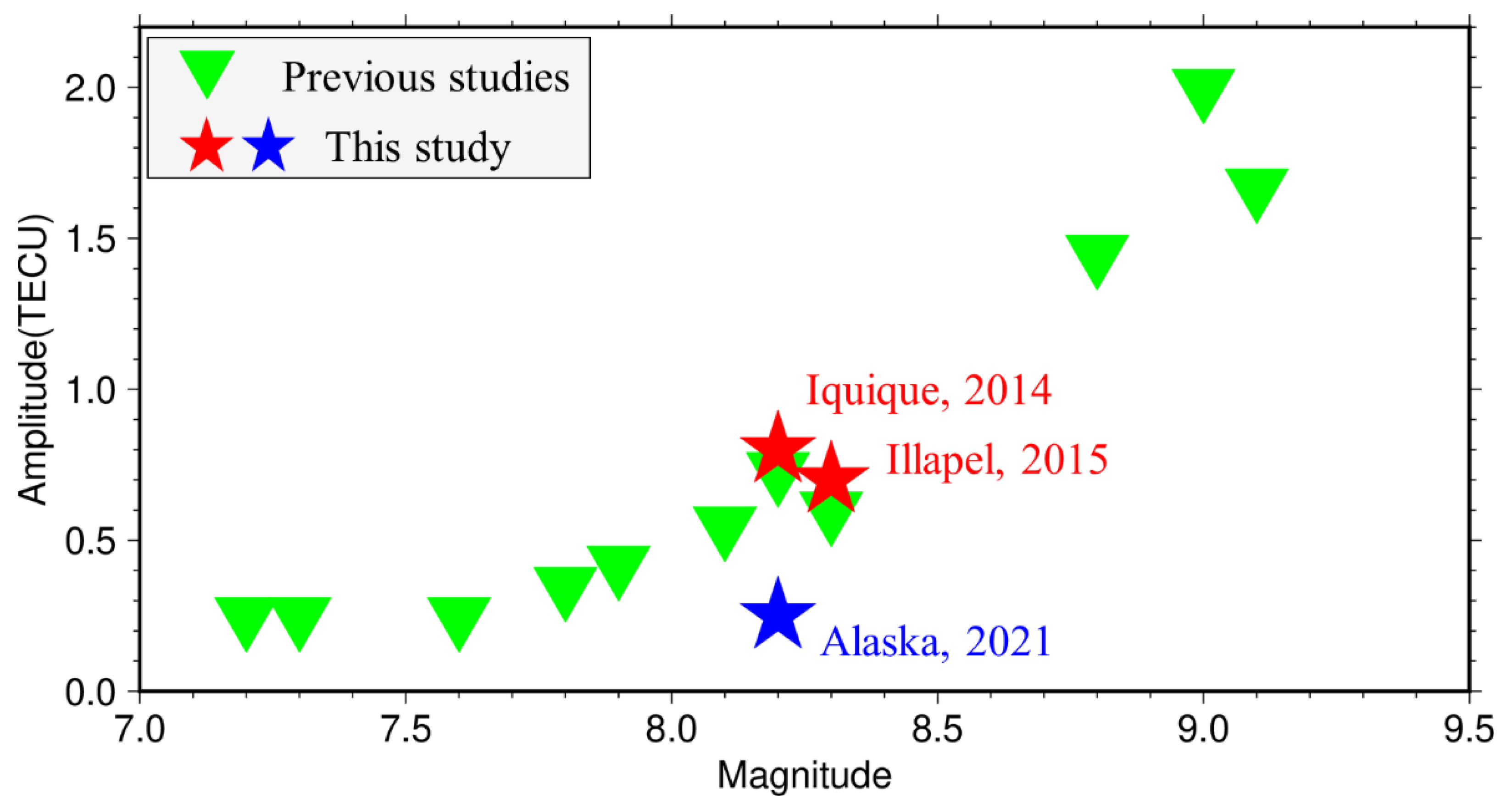
This study #1	1 April 2014	23:46:47	−19.61, −70.77	25.0	8.2	0.8	4.63
This study #2	16 September 2015	22:54:32	−31.57, −71.60	22.4	8.3	0.7	13.60
This study #3	29 July 2021	06:15:47	55.33, −157.84	32.2	8.2	0.25	0.50

.

According to Table 1, the amplitude of TEC disturbances versus the magnitude of earthquakes is shown in Figure 7. The statistical regularity of the reference events supports that quakes with M_w 8.1–M_w 8.3 usually cause ionospheric disturbances of 0.4–0.7 TECU, such as the three events on 4 October 1994 (M_w 8.1), 25 September 2003 (M_w 8.3), and 15 November 2006 (M_w 8.2), and all events caused devastating tsunamis. This result is consistent with the CIDs amplitude and the range of seawater fluctuations we obtained in the Chile events (red stars in Figure 7). With the same magnitude, however, the Alaska event did not produce the expected CIDs amplitude and tsunami water height (blue star in Figure 7 significantly deviate downward). It would be reasonable to consider that this incident is unlikely to produce a destructive tsunami. Using the correlation between the disturbance amplitude and earthquake magnitude, we successfully distinguish the possibility of the tsunami induced by the three earthquakes and provide a basis for the rapid identification of the tsunami potential.

We further explore the relationship of the TEC response with tsunami potential by analyzing the spatial dynamics of the disturbance. The top panels in Figure 8 show screenshots of the CID maps of the Iquique earthquake, and the near -field CIDs exhibit concentric and anisotropic wavefronts to the north and south of the source. The disturbances in the east–west direction are smaller than in the north–south direction, which may be related to the sparse distribution of ground sites in these areas. The middle panels in Figure 8 describe the CIDs that follow the Illapel event. The disturbances are concentrated in the NWN of the epicenter and barely perturbed in the southern sky. This may be because the rupture direction of the earthquake is mainly along the NWN [51,52]. Moreover, the ionospheric electron movement in the southern hemisphere is affected by the Lorentz force, implying that the propagation to the poles may be inhibited [11].

Overall, the propagation directions of the disturbances of the Iquique and Illapel earthquakes tend to rupture towards the shallow portion of the megathrust. Considering that the rigidity of the shallow sediments in this area is low and it is easy to induce relatively large seafloor uplifts, the two earthquakes in Chile both produced destructive tsunamis. On the contrary, the bottom panel of Figure 8 shows that the CIDs generated by the Alaska earthquake are mainly concentrated in the east-northeast of the epicenter, which probabilistically ruptured a deeper portion of the megathrust. In this scenario, the amount of slip produced is significantly smaller than that of the Chilean subduction zone, although it maintains the same moment magnitude. In addition, the focal depth of the Alaska earthquake is deeper than others, and the vertical crustal displacement caused by the rupture is not significant, which explains why there were no damaging tsunamis.

5. Conclusions

Using GNSS observations, we obtained an ionospheric response to the 2014 M_w 8.2 Iquique, 2015 M_w 8.3 Illapel, and 2021 M_w 8.2 Alaska megathrusts. We specially focused on the AGWs that can be quickly (~10 min) identified in the ionosphere, which are related to the vertical component of co-seismic crustal deformation. Our results show a systematically lower CID magnitude associated with the 2021 M_w 8.2 Alaska event, thus implying a weaker seafloor uplift and tsunami potential. Our work demonstrates that the CIDs could be input as auxiliary observation information into the existing tsunami warning system to improve the robustness of rapid tsunami warnings and guard against false alarms.

Finally, it is important to note that the IGWs that come later directly reflect the tsunami characteristics and should be taken for tsunami confirmation. Moreover, we only focus on tsunami potential assessment, and significant AGWs caused by continental events such as the 2015 M_w 7.8 Nepal earthquake should be immediately ruled out for consideration in practice based on its epicenter location. While our work provides another case besides the well demonstrated 2010 M_w 7.8 Mentawai event, more case studies are needed to build a rigorous CID approach for tsunami early warning systems.

References

- Sobolev, S.V.; Babeyko, A.Y.; Wang, R.; Hoechner, A.; Galas, R.; Rothacher, M.; Sein, D.V.; Schroter, J.; Lauterjung, J.; Subarya, C. Tsunami early warning using GPS-Shield arrays. J. Geophys. Res. Solid Earth 2007, 112, B08415. [Google Scholar] [CrossRef]
- Song, Y.T. Detecting tsunami genesis and scales directly from coastal GPS stations. Geophys. Res. Lett. 2007, 34, L19602. [Google Scholar] [CrossRef] [Green Version]
- Hooper, A.; Pietrzak, J.; Simons, W.; Cui, H.; Riva, R.; Naeije, M.; van Scheltinga, A.T.; Schrama, E.; Stelling, G.; Socquet, A. Importance of horizontal seafloor motion on tsunami height for the 2011 Mw = 9.0 Tohoku-Oki earthquake. Earth Planet. Sci. Lett. 2013, 361, 469–479. [Google Scholar] [CrossRef]
- Kanamori, H.; Rivera, L. Source inversion of W phase: Speeding up seismic tsunami warning. Geophys. J. Int. 2008, 175, 222–238. [Google Scholar] [CrossRef]
- Melgar, D.; Bock, Y. Near-field tsunami models with rapid earthquake source inversions from land- and ocean-based observations: The potential for forecast and warning. J. Geophys. Res. Solid Earth 2013, 118, 5939–5955. [Google Scholar] [CrossRef]
- Chen, K.J.; Liu, Z.; Song, Y.T. Automated GNSS and Teleseismic Earthquake Inversion (AutoQuake Inversion) for Tsunami Early Warning: Retrospective and Real-Time Results. Pure Appl. Geophys. 2020, 177, 1403–1423. [Google Scholar] [CrossRef] [Green Version]
- Government Accountability Office. Tsunami Preparedness: Federal and State Partners Collaborate to Help Communities Reduce Potential Impacts, but Significant Challenges Remain; Government Accountability Office, Ed.; U.S. Government Printing Office: Washington, DC, USA, 2006; Volume 06-519, pp. 1–65.
- Dautermann, T.; Calais, E.; Lognonne, P.; Mattioli, G.S. Lithosphere-atmosphere-ionosphere coupling after the 2003 explosive eruption of the Soufriere Hills Volcano, Montserrat. Geophys. J. Int. 2009, 179, 1537–1546. [Google Scholar] [CrossRef] [Green Version]
- Rakoto, V.; Lognonne, P.; Rolland, L.; Coisson, P. Tsunami Wave Height Estimation from GPS-Derived Ionospheric Data. J. Geophys. Res. Space Phys. 2018, 123, 4329–4348. [Google Scholar] [CrossRef]
- Rakoto, V.; Lognonne, P.; Rolland, L. Tsunami modeling with solid Earth-ocean-atmosphere coupled normal modes. Geophys. J. Int. 2017, 211, 1119–1138. [Google Scholar] [CrossRef]
- Artru, J.; Ducic, V.; Kanamori, H.; Lognonne, P.; Murakami, M. Ionospheric detection of gravity waves induced by tsunamis. Geophys. J. Int. 2005, 160, 840–848. [Google Scholar] [CrossRef] [Green Version]
- Afraimovich, E.L.; Terekhov, A.I.; Udodov, M.Y.; Fridman, S.V. Refraction Distortions of Transionospheric Radio Signals Caused by Changes in a Regular Ionosphere and by Traveling Ionospheric Disturbances. J. Atmos. Terr. Phys. 1992, 54, 1013–1020. [Google Scholar] [CrossRef]
- Manta, F.; Occhipinti, G.; Feng, L.J.; Hill, E.M. Rapid identification of tsunamigenic earthquakes using GNSS ionospheric sounding. Sci. Rep. 2020, 10, 11054. [Google Scholar] [CrossRef] [PubMed]
- Satake, K.; Nishimura, Y.; Putra, P.S.; Gusman, A.R.; Sunendar, H.; Fujii, Y.; Tanioka, Y.; Latief, H.; Yulianto, E. Tsunami Source of the 2010 Mentawai, Indonesia Earthquake Inferred from Tsunami Field Survey and Waveform Modeling. Pure Appl. Geophys. 2013, 170, 1567–1582. [Google Scholar] [CrossRef] [Green Version]
- Tu, R.; Zhang, H.; Ge, M.; Huang, G. A real-time ionospheric model based on GNSS Precise Point Positioning. Adv. Space Res. 2013, 52, 1125–1134. [Google Scholar] [CrossRef]
- Brunini, C.; Azpilicueta, F.J. Accuracy assessment of the GPS-based slant total electron content. J. Geod. 2009, 83, 773–785. [Google Scholar] [CrossRef]
- Jin, S.G.; Occhipinti, G.; Jin, R. GNSS ionospheric seismology: Recent observation evidences and characteristics. Earth-Sci. Rev. 2015, 147, 54–64. [Google Scholar] [CrossRef]
- Klobuchar, J.A. Ionospheric Time-Delay Algorithm for Single-Frequency GPS Users. IEEE Trans. Aerosp. Electron. Syst. 1987, 23, 325–331. [Google Scholar] [CrossRef]
- Liu, J.Y.; Tsai, H.F.; Lin, C.H.; Kamogawa, M.; Chen, Y.I.; Huang, B.S.; Yu, S.B.; Yeh, Y.H. Coseismic ionospheric disturbances triggered by the Chi-Chi earthquake. J. Geophys. Res. Space Phys. 2010, 115, A08303. [Google Scholar] [CrossRef]
- Liu, J.Y.; Lin, C.Y.; Tsai, Y.L.; Liu, T.C.; Hattori, K.; Sun, Y.Y.; Wu, T.R. Ionospheric GNSS Total Electron Content for Tsunami Warning. J. Earthq. Tsunami 2019, 13, 1941007. [Google Scholar] [CrossRef]
- Li, Z.; Wang, N.; Liu, A.; Yuan, Y.; Wang, L.; Hernández-Pajares, M.; Krankowski, A.; Yuan, H. Status of CAS global ionospheric maps after the maximum of solar cycle 24. Satell. Navig. 2021, 2, 19. [Google Scholar] [CrossRef]
- Coster, A.; Williams, J.; Weatherwax, A.; Rideout, W.; Herne, D. Accuracy of GPS total electron content: GPS receiver bias temperature dependence. Radio Sci. 2013, 48, 190–196. [Google Scholar] [CrossRef]
- Kong, J.; Yao, Y.B.; Zhou, C.; Liu, Y.; Zhai, C.Z.; Wang, Z.M.; Liu, L. Tridimensional reconstruction of the Co-Seismic Ionospheric Disturbance around the time of 2015 Nepal earthquake. J. Geod. 2018, 92, 1255–1266. [Google Scholar] [CrossRef]
- Nicolls, M.J.; Kelley, M.C.; Coster, A.J.; Gonzalez, S.A.; Makela, J.J. Imaging the structure of a large-scale TID using ISR and TEC data. Geophys. Res. Lett. 2004, 31, L09812. [Google Scholar] [CrossRef]
- Perevalova, N.P.; Sankov, V.A.; Astafyeva, E.I.; Zhupityaeva, A.S. Threshold magnitude for Ionospheric TEC response to earthquakes. J. Atmos. Sol.-Terr. Phys. 2014, 108, 77–90. [Google Scholar] [CrossRef]
- Richmond, A.D.; Matsushita, S. Thermospheric Response to a Magnetic Substorm. J. Geophys. Res. Space Phys. 1975, 80, 2839–2850. [Google Scholar] [CrossRef]
- Occhipinti, G.; Kherani, E.A.; Lognonne, P. Geomagnetic dependence of ionospheric disturbances induced by tsunamigenic internal gravity waves. Geophys. J. Int. 2008, 173, 753–765. [Google Scholar] [CrossRef]
- Dautermann, T.; Calais, E.; Mattioli, G.S. Global Positioning System detection and energy estimation of the ionospheric wave caused by the 13 July 2003 explosion of the Soufriere Hills Volcano, Montserrat. J. Geophys. Res. Solid Earth 2009, 114, B02202. [Google Scholar] [CrossRef]
- Shrivastava, M.N.; Maurya, A.K.; Gonzalez, G.; Sunil, P.S.; Gonzalez, J.; Salazar, P.; Aranguiz, R. Tsunami detection by GPS-derived ionospheric total electron content. Sci. Rep. 2021, 11, 12978. [Google Scholar] [CrossRef]
- Catalan, P.A.; Aranguiz, R.; Gonzalez, G.; Tomita, T.; Cienfuegos, R.; Gonzalez, J.; Shrivastava, M.N.; Kumagai, K.; Mokrani, C.; Cortes, P.; et al. The 1 April 2014 Pisagua tsunami: Observations and modeling. Geophys. Res. Lett. 2015, 42, 2918–2925. [Google Scholar] [CrossRef]
- Aranguiz, R.; Gonzalez, G.; Gonzalez, J.; Catalan, P.A.; Cienfuegos, R.; Yagi, Y.; Okuwaki, R.; Urra, L.; Contreras, K.; Del Rio, I.; et al. The 16 September 2015 Chile Tsunami from the Post-Tsunami Survey and Numerical Modeling Perspectives. Pure Appl. Geophys. 2016, 173, 333–348. [Google Scholar] [CrossRef]
- Astafyeva, E.; Heki, K.; Kiryushkin, V.; Afraimovich, E.; Shalimov, S. Two-mode long-distance propagation of coseismic ionosphere disturbances. J. Geophys. Res. Space Phys. 2009, 114, A10307. [Google Scholar] [CrossRef] [Green Version]
- Afraimovich, E.L.; Ding, F.; Kiryushkin, V.V.; Astafyeva, E.I.; Jin, S.G.; Sankov, V.A. TEC response to the 2008 Wenchuan Earthquake in comparison with other strong earthquakes. Int. J. Remote Sens. 2010, 31, 3601–3613. [Google Scholar] [CrossRef] [Green Version]
- Astafyeva, E.; Heki, K. Dependence of waveform of near-field coseismic ionospheric disturbances on focal mechanisms. Earth Planets Space 2009, 61, 939–943. [Google Scholar] [CrossRef] [Green Version]
- Liu, H.T.; Zhang, K.K.; Imtiaz, N.; Song, Q.; Zhang, Y. Relating Far-Field Coseismic Ionospheric Disturbances to Geological Structures. J. Geophys. Res. Space Phys. 2021, 126, e2021JA029209. [Google Scholar] [CrossRef]
- Astafyeva, E. Ionospheric Detection of Natural Hazards. Rev. Geophys. 2019, 57, 1265–1288. [Google Scholar] [CrossRef]
- Reddy, C.D.; Sunil, A.S.; Gonzalez, G.; Shrivastava, M.N.; Moreno, M. Near-field co-seismic ionospheric response due to the northern Chile Mw 8.1 Pisagua earthquake on April 1, 2014 from GPS observations. J. Atmos. Sol.-Terr. Phys. 2015, 134, 1–8. [Google Scholar] [CrossRef]
- Occhipinti, G.; Rolland, L.; Lognonne, P.; Watada, S. From Sumatra 2004 to Tohoku-Oki 2011: The systematic GPS detection of the ionospheric signature induced by tsunamigenic earthquakes. J. Geophys. Res. Space Phys. 2013, 118, 3626–3636. [Google Scholar] [CrossRef]
- Nishitani, N.; Ogawa, T.; Otsuka, Y.; Hosokawa, K.; Hori, T. Propagation of large amplitude ionospheric disturbances with velocity dispersion observed by the SuperDARN Hokkaido radar after the 2011 off the Pacific coast of Tohoku Earthquake. Earth Planets Space 2011, 63, 891–896. [Google Scholar] [CrossRef] [Green Version]
- Cahyadi, M.N.; Heki, K. Coseismic ionospheric disturbance of the large strike-slip earthquakes in North Sumatra in 2012: M-w dependence of the disturbance amplitudes. Geophys. J. Int. 2015, 200, 116–129. [Google Scholar] [CrossRef] [Green Version]
- Zettergren, M.D.; Snively, J.B. Ionospheric response to infrasonic-acoustic waves generated by natural hazard events. J. Geophys. Res. Space Phys. 2015, 120, 8002–8024. [Google Scholar] [CrossRef] [Green Version]
- Nishida, K.; Kobayashi, N.; Fukao, Y. Resonant oscillations between the solid Earth and the atmosphere. Science 2000, 287, 2244–2246. [Google Scholar] [CrossRef] [PubMed]
- Saito, A.; Tsugawa, T.; Otsuka, Y.; Nishioka, M.; Iyemori, T.; Matsumura, M.; Saito, S.; Chen, C.H.; Goi, Y.; Choosakul, N. Acoustic resonance and plasma depletion detected by GPS total electron content observation after the 2011 off the Pacific coast of Tohoku Earthquake. Earth Planets Space 2011, 63, 863–867. [Google Scholar] [CrossRef] [Green Version]
- Richmond, A.D. Gravity-Wave Generation, Propagation, and Dissipation in Thermosphere. J. Geophys. Res. Space Phys. 1978, 83, 4131–4145. [Google Scholar] [CrossRef]
- Mao, T.; Wang, J.S.; Yang, G.L.; Yu, T.; Ping, J.S.; Suo, Y.C. Effects of typhoon Matsa on ionospheric TEC. Chin. Sci. Bull. 2010, 55, 712–717. [Google Scholar] [CrossRef]
- Reddy, C.D.; Shrivastava, M.N.; Seemala, G.K.; Gonzalez, G.; Baez, J.C. Ionospheric Plasma Response to M (w) 8.3 Chile Illapel Earthquake on September 16, 2015. Pure Appl. Geophys. 2016, 173, 1451–1461. [Google Scholar] [CrossRef]
- Wan, X.; Xiong, C.; Gao, S.Z.; Huang, F.Q.; Liu, Y.W.; Aa, E.C.; Yin, F.; Cai, H.T. The nighttime ionospheric response and occurrence of equatorial plasma irregularities during geomagnetic storms: A case study. Satell. Navig. 2021, 2, 23. [Google Scholar] [CrossRef]
- Bhattacharya, S.; Dubey, S.; Tiwari, R.; Purohit, P.K.; Gwal, A.K. Effect of magnetic activity on ionospheric time delay at low latitude. J. Astrophys. Astron. 2008, 29, 269–274. [Google Scholar] [CrossRef]
- Bartels, J.; Veldkamp, J. International Data on Magnetic Disturbances, 4th Quarter, 1955. J. Geophys. Res. 1956, 61, 285–292. [Google Scholar]
- Astafyeva, E.; Shalimov, S.; Olshanskaya, E.; Lognonne, P. Ionospheric response to earthquakes of different magnitudes: Larger quakes perturb the ionosphere stronger and longer. Geophys. Res. Lett. 2013, 40, 1675–1681. [Google Scholar] [CrossRef] [Green Version]
- Ye, L.L.; Lay, T.; Kanamori, H.; Koper, K.D. Reply to: Comment by Rodrigo Cienfuegos on “Rapidly Estimated Seismic Source Parameters for the 16 September 2015 Illapel, Chile, Mw 8.3 Earthquake” by Lingling Ye, Thorne Lay, Hiroo Kanamori, and Keith D. Koper. Pure Appl. Geophys. 2019, 176, 2753. [Google Scholar] [CrossRef] [Green Version]
- Heidarzadeh, M.; Murotani, S.; Satake, K.; Ishibe, T.; Gusman, A.R. Source model of the 16 September 2015 Illapel, Chile, M-w 8.4 earthquake based on teleseismic and tsunami data. Geophys. Res. Lett. 2016, 43, 643–650. [Google Scholar] [CrossRef] [Green Version]