
Ocean Color Remote Sensing of Suspended Sediments along a Continuum from Rivers to River Plumes: Concentration, Transport, Fluxes and Dynamics


Abstract
:
1. Introduction
2. Materials and Methods
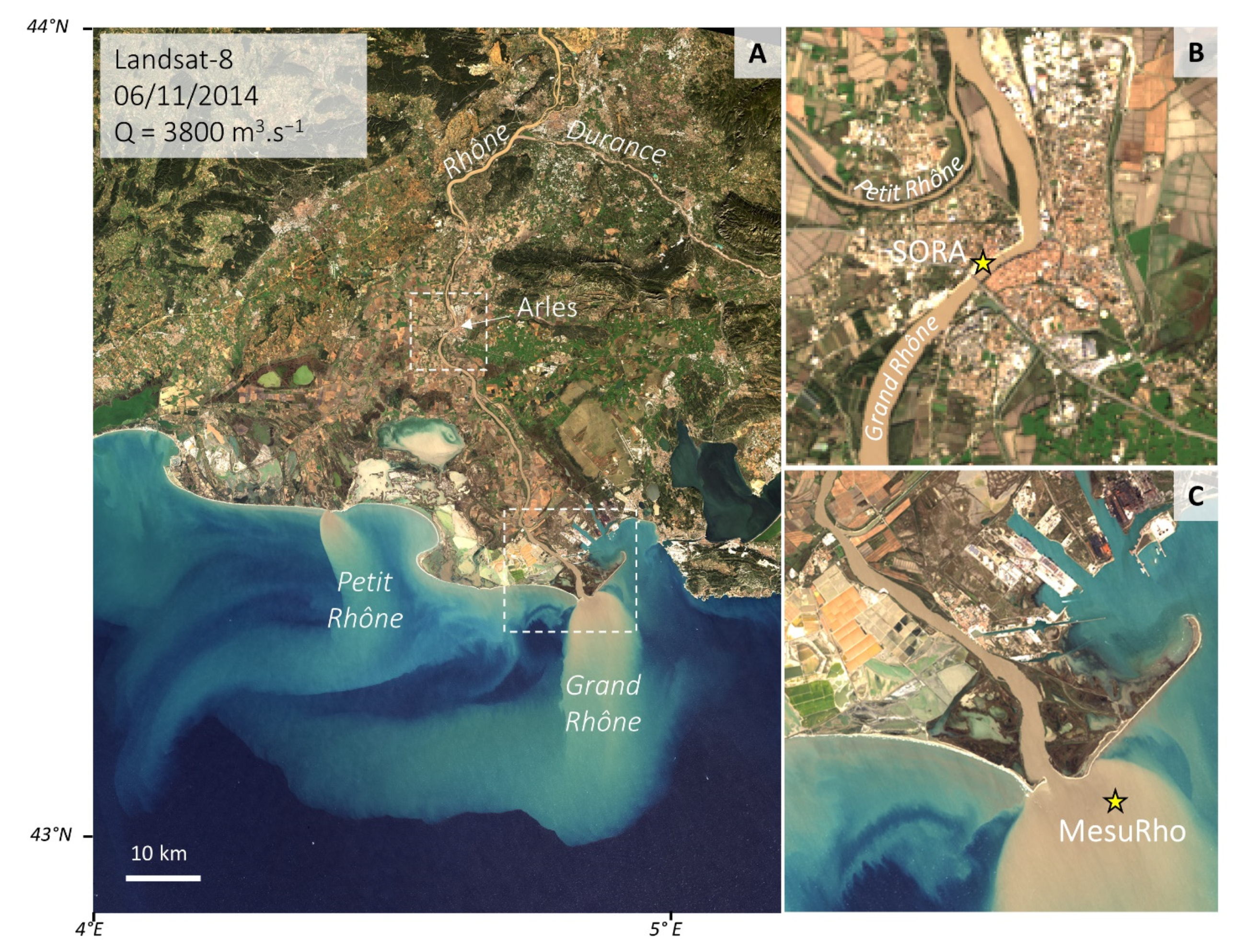
2.1. Study Area and Context
2.2. Dataset
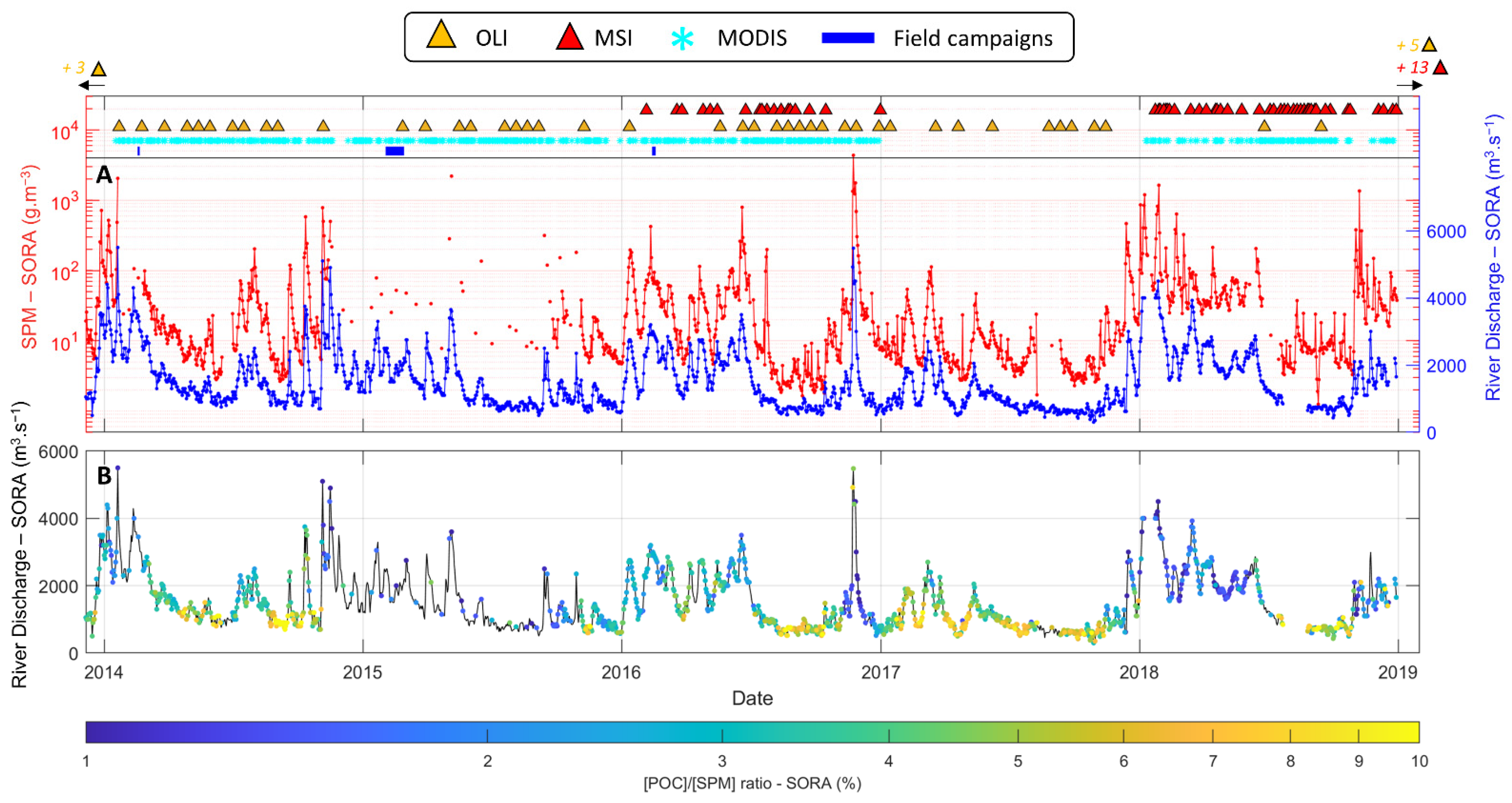
2.2.1. In Situ Measurements from the SORA Station (Arles)

2.2.2. In Situ Measurements from Field Campaigns
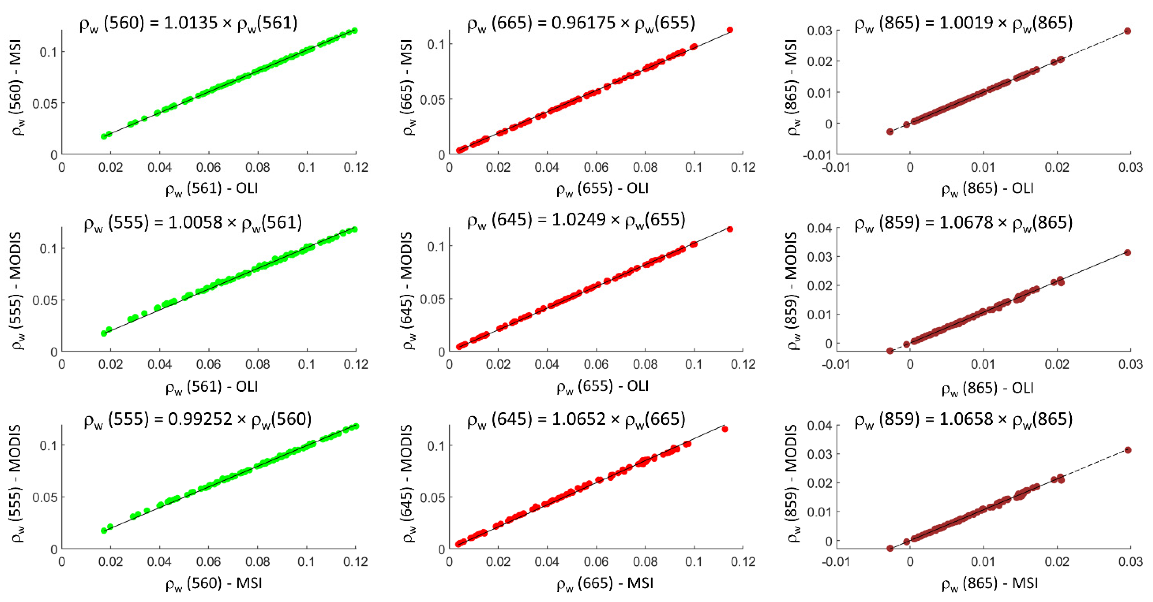
2.2.3. Satellite Dataset
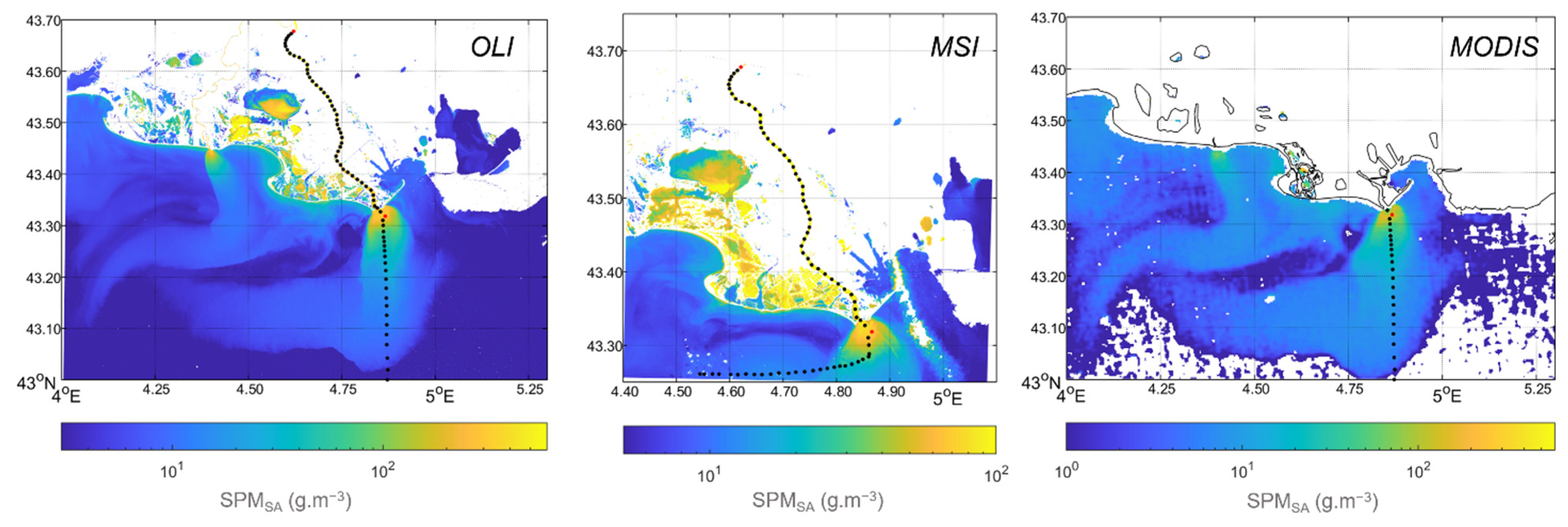
- The OLI sensor on the Landsat-8 (L8) polar-orbiting satellite platform launched in 2013. This sensor provides multispectral data with a high spatial resolution of 30 m and a temporal resolution of 16 days;
- The MSI sensors on the Sentinel-2 A (S2-A) and B (S2-B) European polar-orbiting satellite platforms launched in 2015 and 2017, respectively, which provide high spatial resolution data (10 to 60 m) and a temporal resolution at the study area latitude of 2–3 days using both satellite platforms;
- The MODIS sensors aboard the polar-orbiting Terra (MODIS-T) and Aqua (MODIS-A) satellite platforms launched in 1999 and 2002, respectively. They provide multispectral data with a revisiting time of one day at the latitude of the study area (thus 2 MODIS images per day with a ~2 h gap between them), with three spatial resolutions of 250 m, 500 m, and 1 km, depending on the spectral band.

| Satellite Dataset | Satellite/Sensors | Used Spectral Bands (nm) | Spatial Resolution (m) | Temporal Resolution (Days) | Atmospheric Correction | Number of Images (N) | Temporal Coverage |
| Landsat-8/OLI | 561 | 30 | 16 | DSF with glint correction [31,32] | 56 | 2013–2018; 2019–2020 (high flooding events only) | |
| 655 | 30 | ||||||
| 865 | 30 | ||||||
| Sentinel-2/MSI | 560 | 10 | 2–3 | DSF with glint correction [31,32] | 86 | 2016; 2018; 2019–2020 (high flooding events only) | |
| 665 | 10 | ||||||
| 865 | 20 | ||||||
| AQUA/MODIS TERRA/MODIS | 555 | 500 | 1 | MUMM [34] or SWIR [35] for highly turbid waters | 1211 | 2014–2016 2018 (AQUA only) | |
| 645 | 250 | ||||||
| 859 | 250 | ||||||
| In situ Dataset | Location | Parameter | Acquisition Method | Temporal Coverage | |||
| SORA station (Arles)–Rhône River | River discharge (m3.s−1) | Autonomous measurements at SORA station: daily averaged measurements and 4 h high frequency measurements during high flooding events (Q > 3000 m3.s−1). | 2005–2020 | ||||
| SORA station (Arles)–Rhône River | SPM concentration (g.m−3) | Autonomous measurements at SORA station: daily sampling and 4 h high frequency sampling during high flooding events (Q > 3000 m3.s−1). | 2005–2020 | ||||
| SORA station (Arles)–Rhône River | POC concentration (g.m−3) | Autonomous measurements at SORA station: daily sampling and 4 h high frequency sampling during high flooding events (Q > 3000 m3.s−1). | 2005–2020 | ||||
| Rhône River plume | SPM concentration (g.m−3) | Sampling during field campaigns. | February 2014 | ||||
| February 2015 | |||||||
| February 2016 | |||||||
| Rhône River plume | Above-water reflectance | Measured with TriOS portable sensor simultaneously with SPM sampling during field campaigns. | February 2014 | ||||
| February 2015 | |||||||
| February 2016 | |||||||
2.3. SPM Switching Algorithm
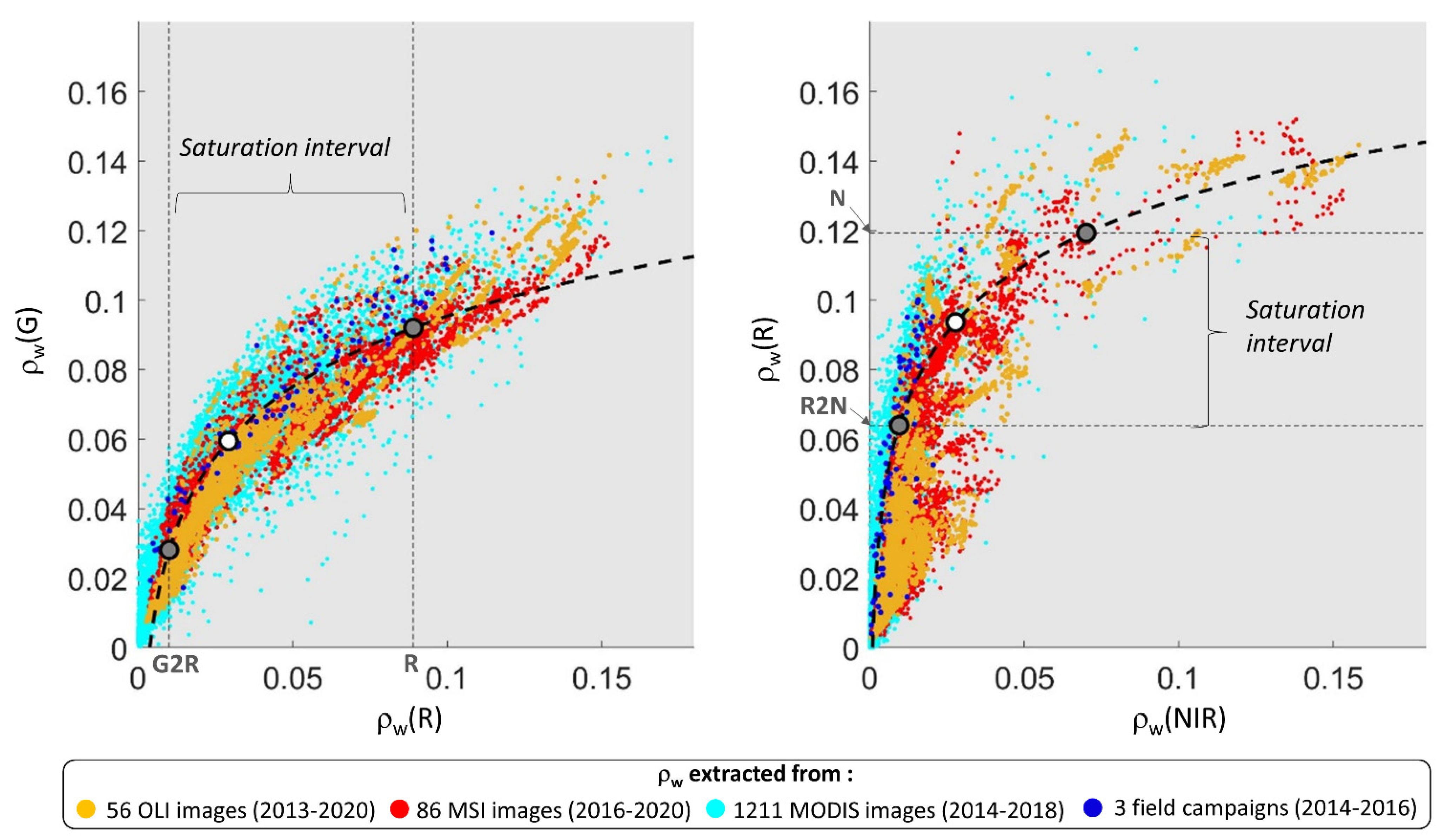
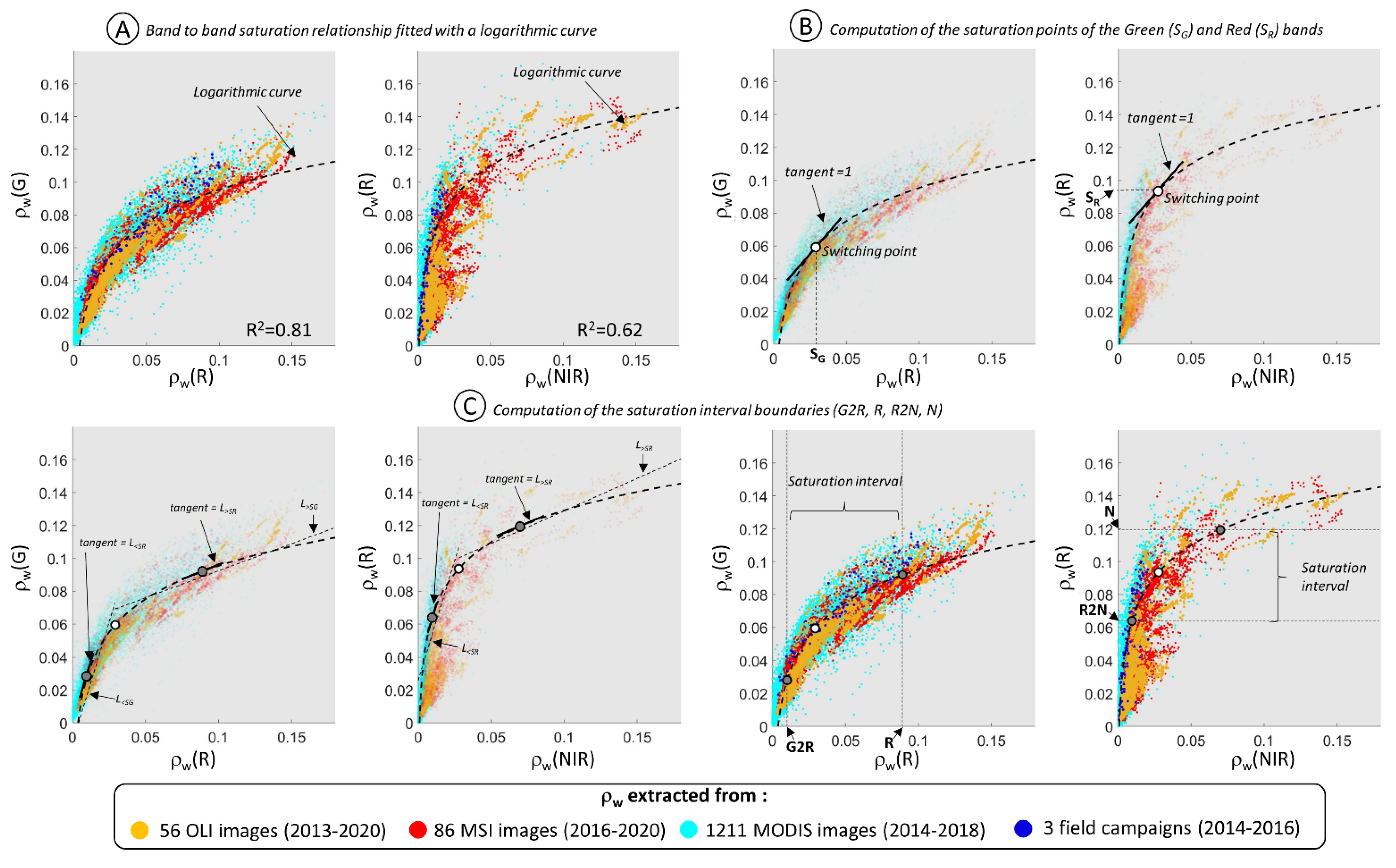
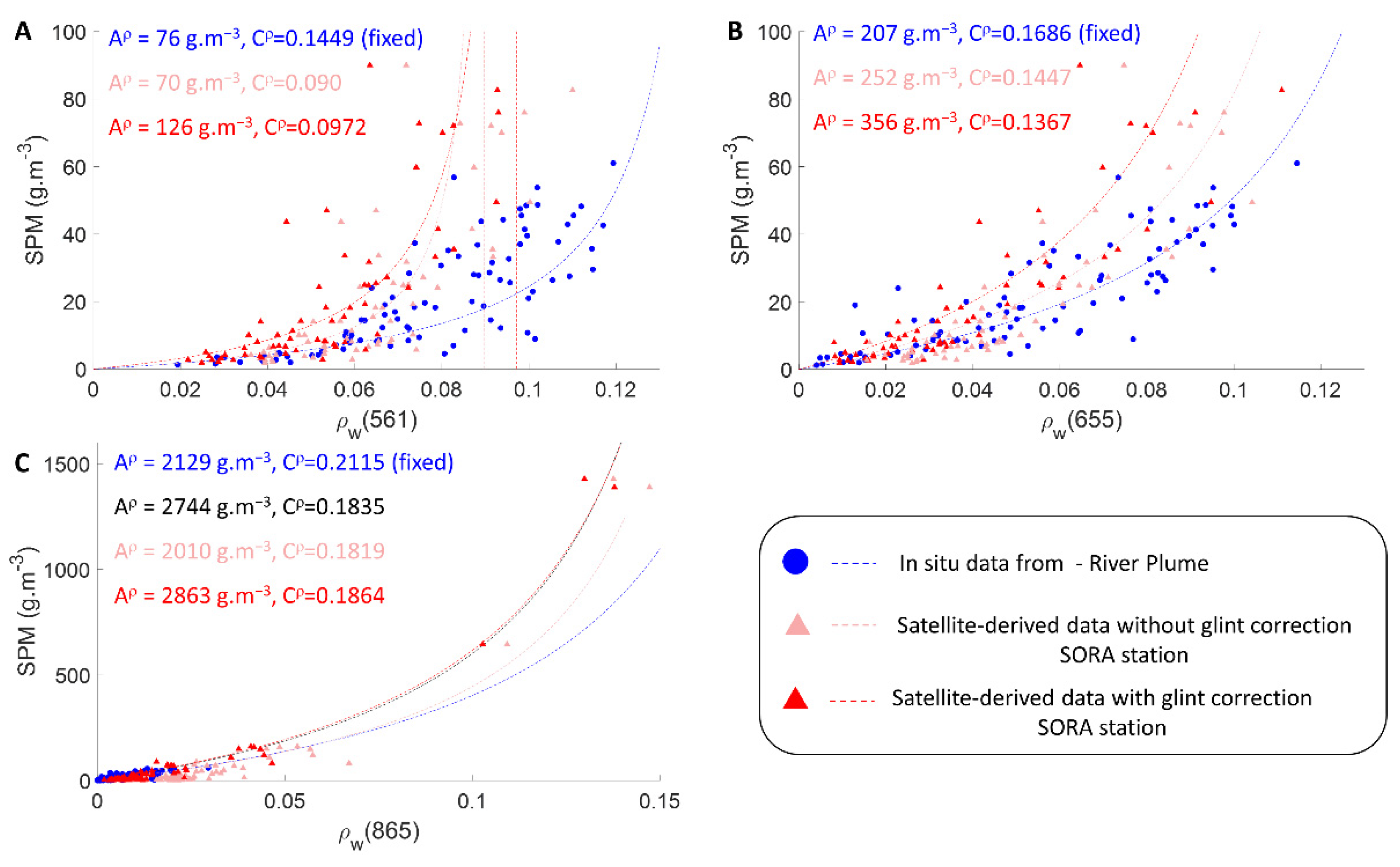
2.3.1. ρw vs. SPM Relationships
2.3.2. SPMSA Concentration Computation Using the Switching Algorithm
2.4. Calculation of the River Plume Surface and SPM Mass
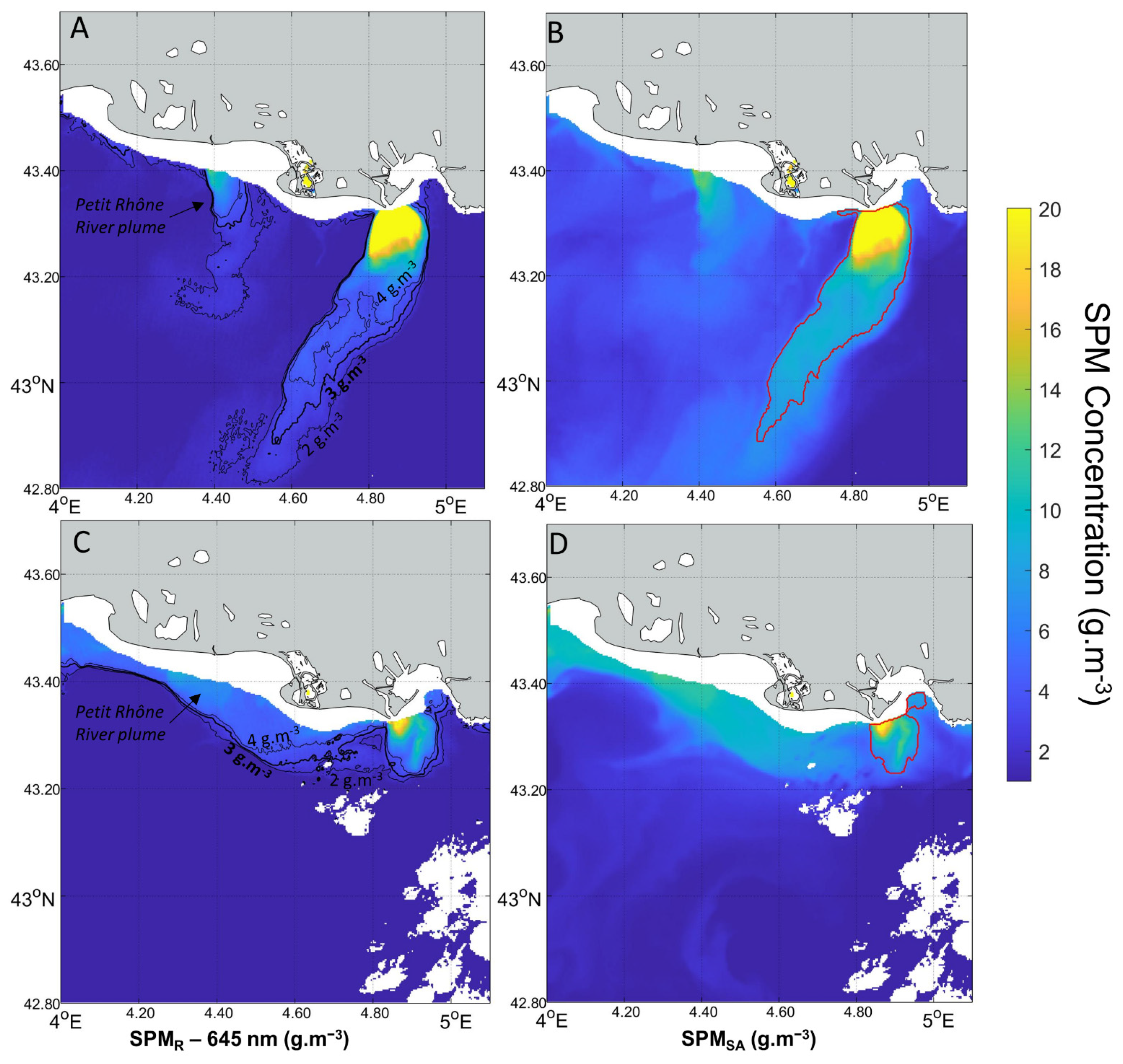
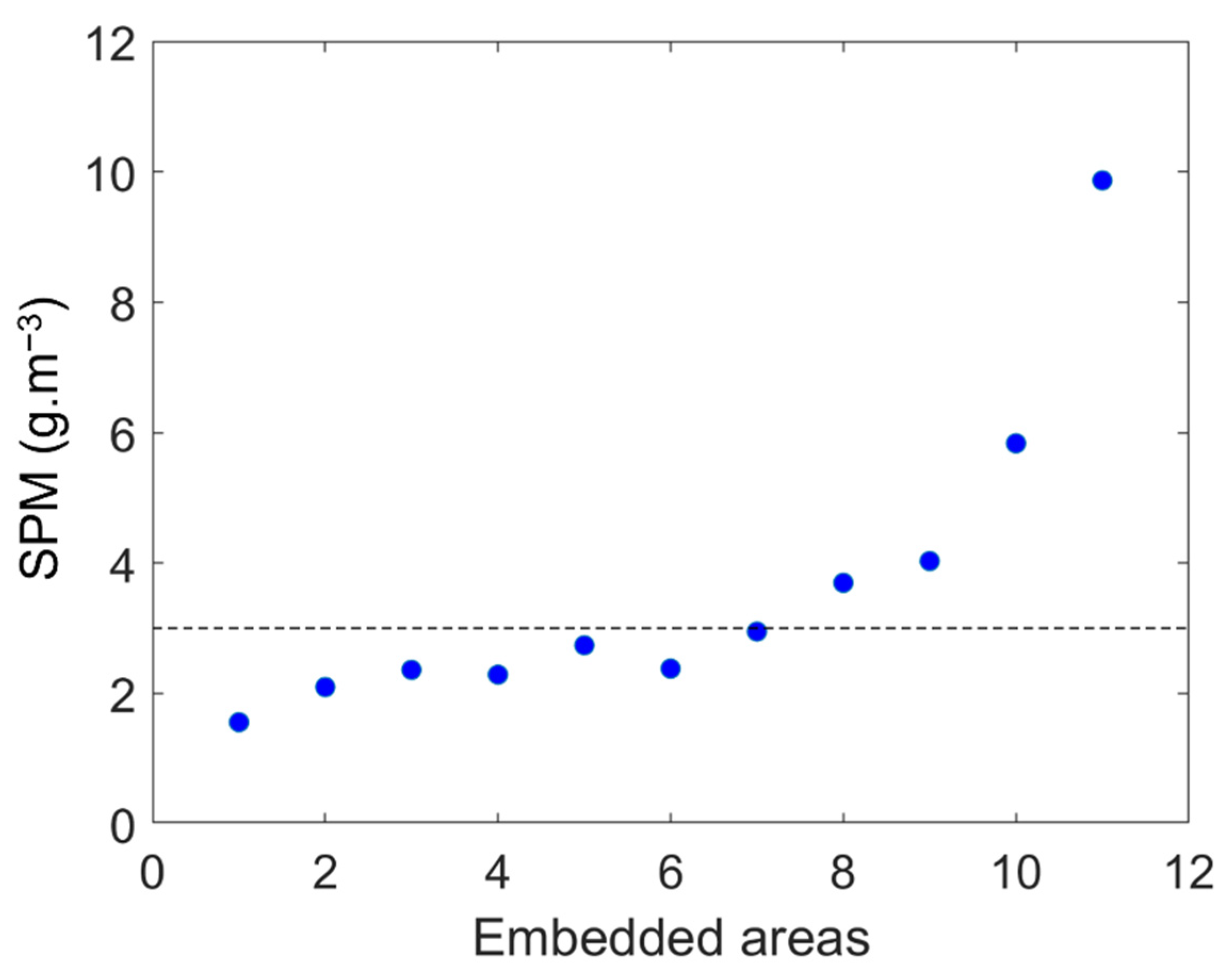
- The identification of the Grand Rhône River plume was completed by selecting the contour with the minimal distance to the river mouth (here defined as the MesuRho platform pixel) lower than 1 km (Figure 5B). When both the Petit Rhône and Grand Rhône River turbid plumes were merged (mainly under southeastern winds), a routine was used to allow the contour to slightly contract (between 3 and 4 g.m−3), using the Chan–Vese active boundaries model [42] in order to separate them as best as possible.
- The plume surface was estimated by summing the number of pixels within its boundary and was converted to area units (in km2) considering the MODIS spatial resolution of 0.25 km.
- The SPM mass within the river plume was estimated assuming a 1 m thickness with a homogeneous SPM concentration. This choice of 1 m thickness was mainly based on the optical depth viewed by the satellite sensor in the red spectral band, e.g., in [11]. The SPMSA concentration of each pixel inside the defined turbid plume boundaries were thus multiplied by pixel volume (area × 1 m) and then summed. Nevertheless, measurements show that the Rhône River surface turbid plume has a thickness varying between 1 and 5 m depending on the wind direction and distance from the coast, and with a sharp decrease in the SPM concentration within the first meters (e.g., [11,23]). The SPM mass computed in this study thus has to be considered a first approximation of the mass of sediment trapped in the surface plume layer.
3. Results
3.1. Validation of the Switching Algorithm
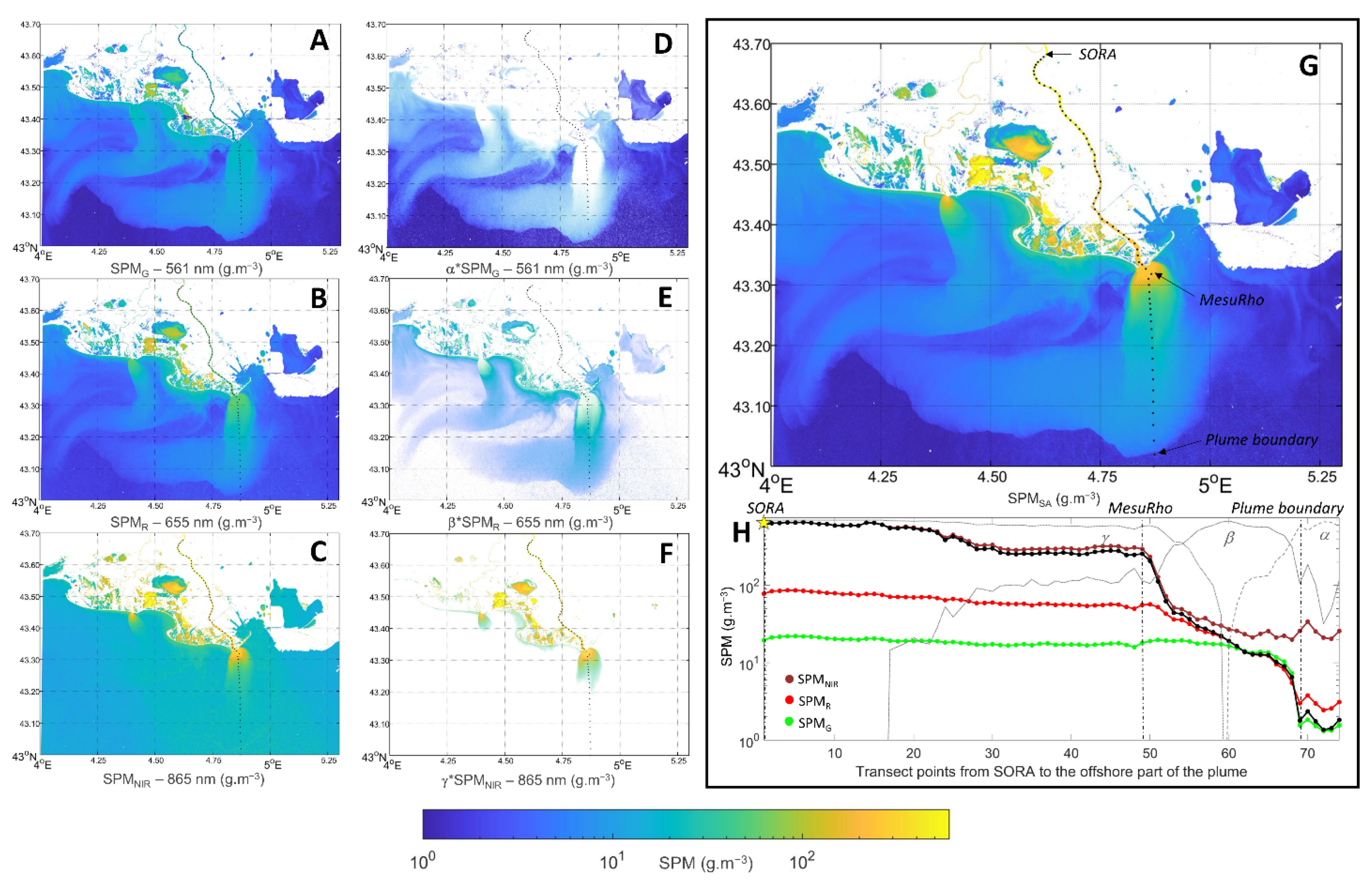
3.1.1. Illustration of the Switching Algorithm Application
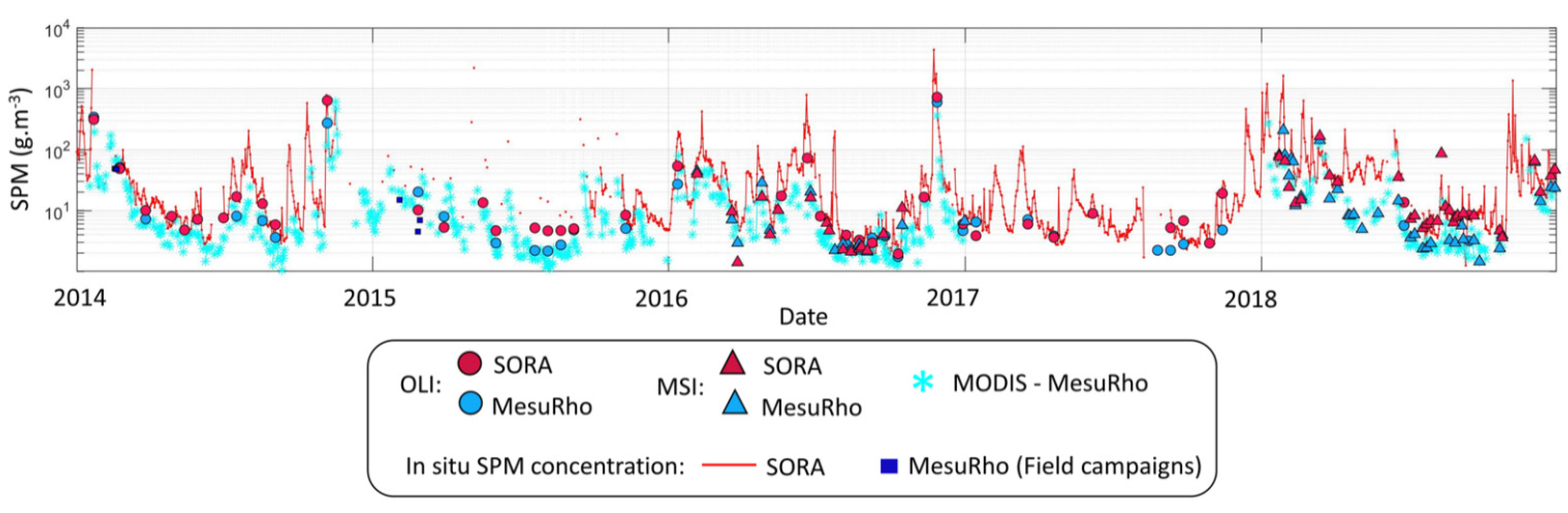
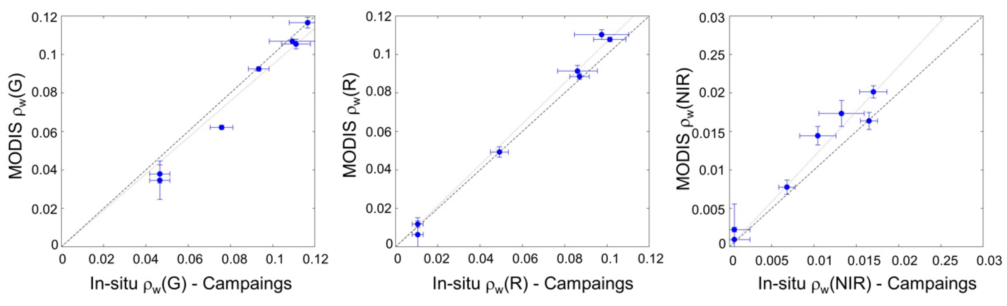
3.1.2. Matchups Validation
3.1.3. SPM Concentration Time Series Using the Switching Algorithm
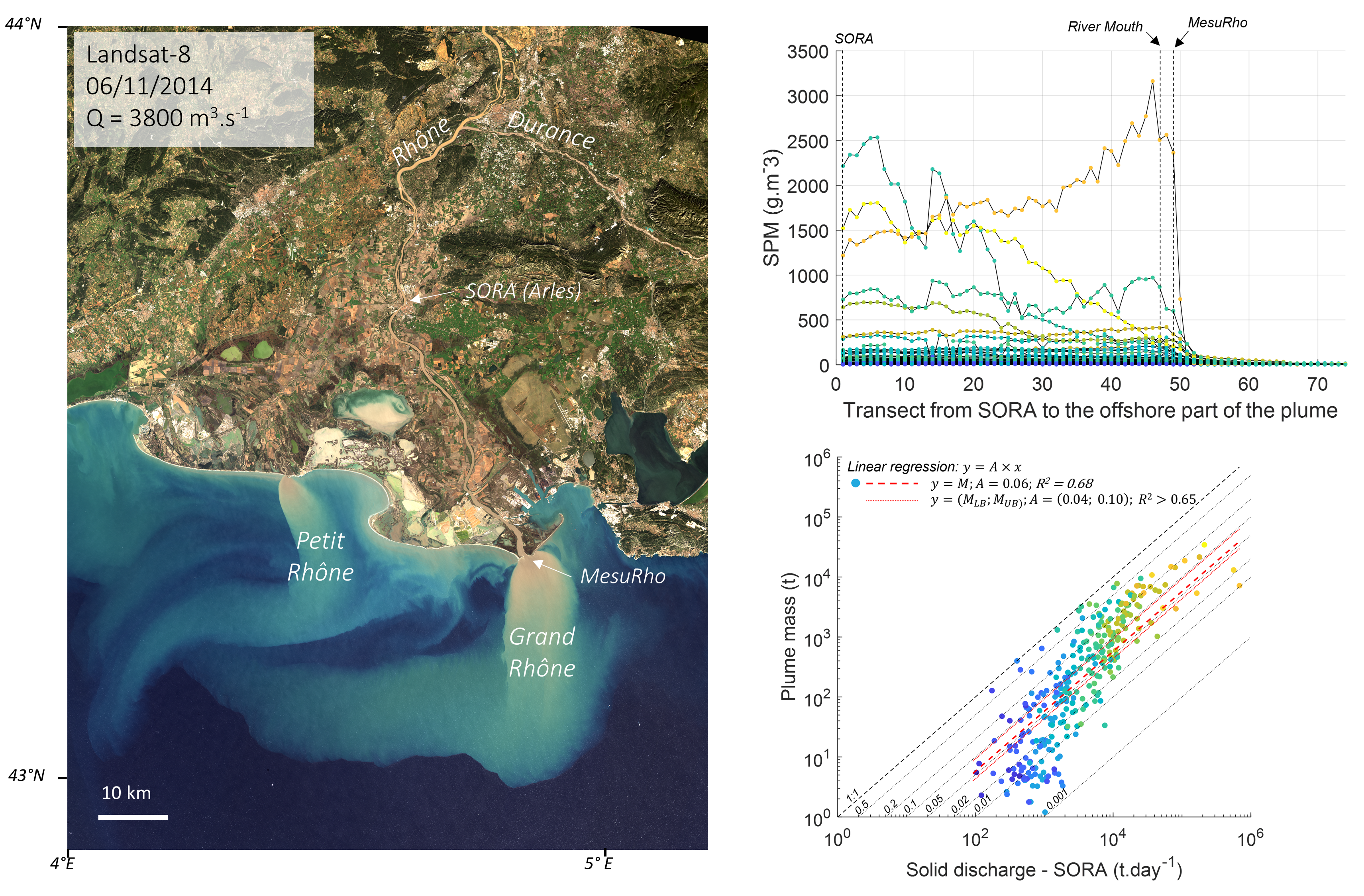
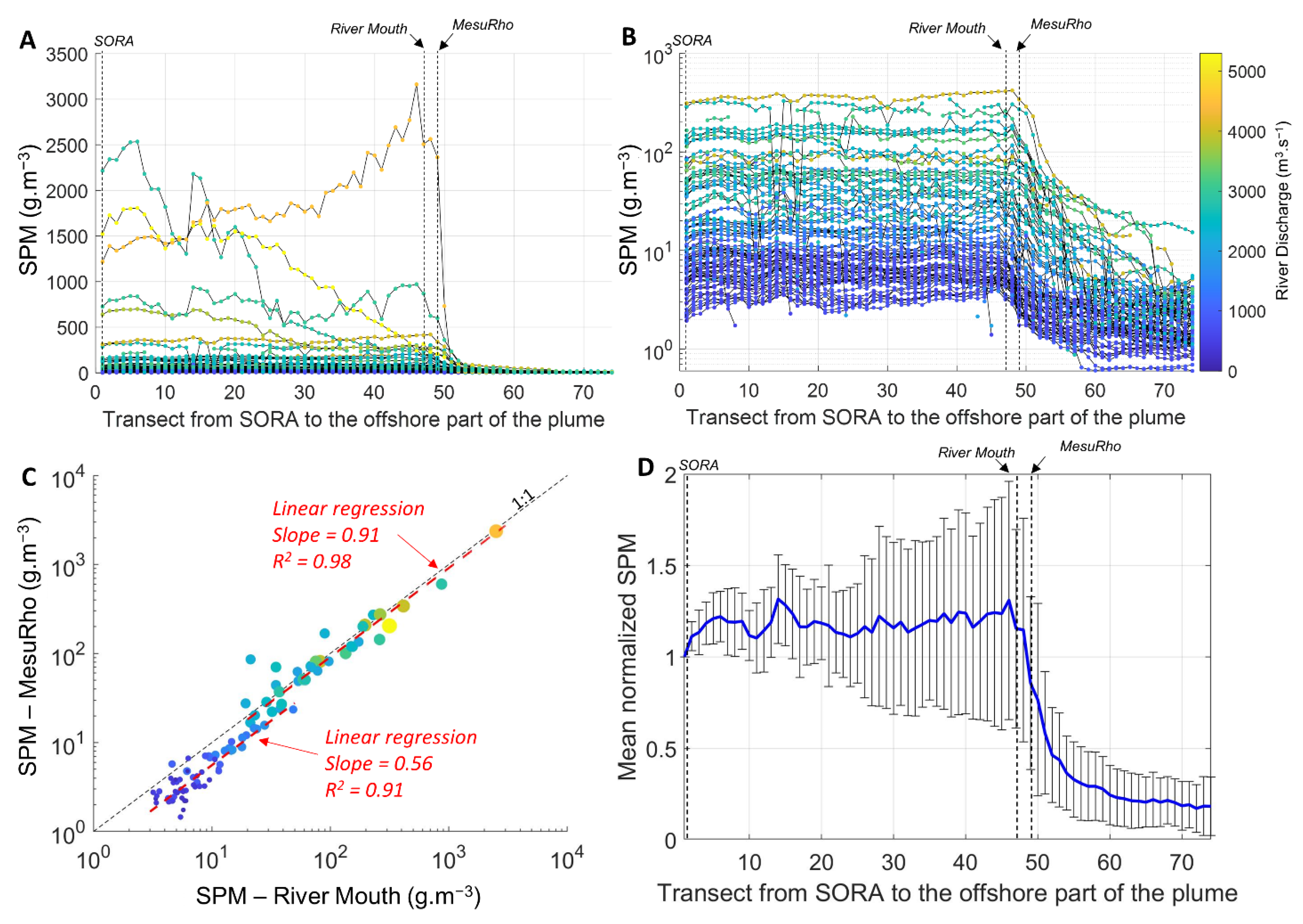
3.2. Sediment Transport from SORA to MesuRho
3.3. Relationships between the Rhône River Discharge, Plume Area, and SPM Mass
3.4. Transfer of Suspended Particulate Matter from the River to the River Plume


4. Discussion
4.1. The Switching SPM Algorithm
4.2. Transport of SPM from the Downstream Part of the River to the Offshore Limits of the River Plume
5. Conclusions
Author Contributions
Funding
Acknowledgments
Conflicts of Interest
Appendix A
Appendix A.1. ρw vs. SPM Concentration Relationships
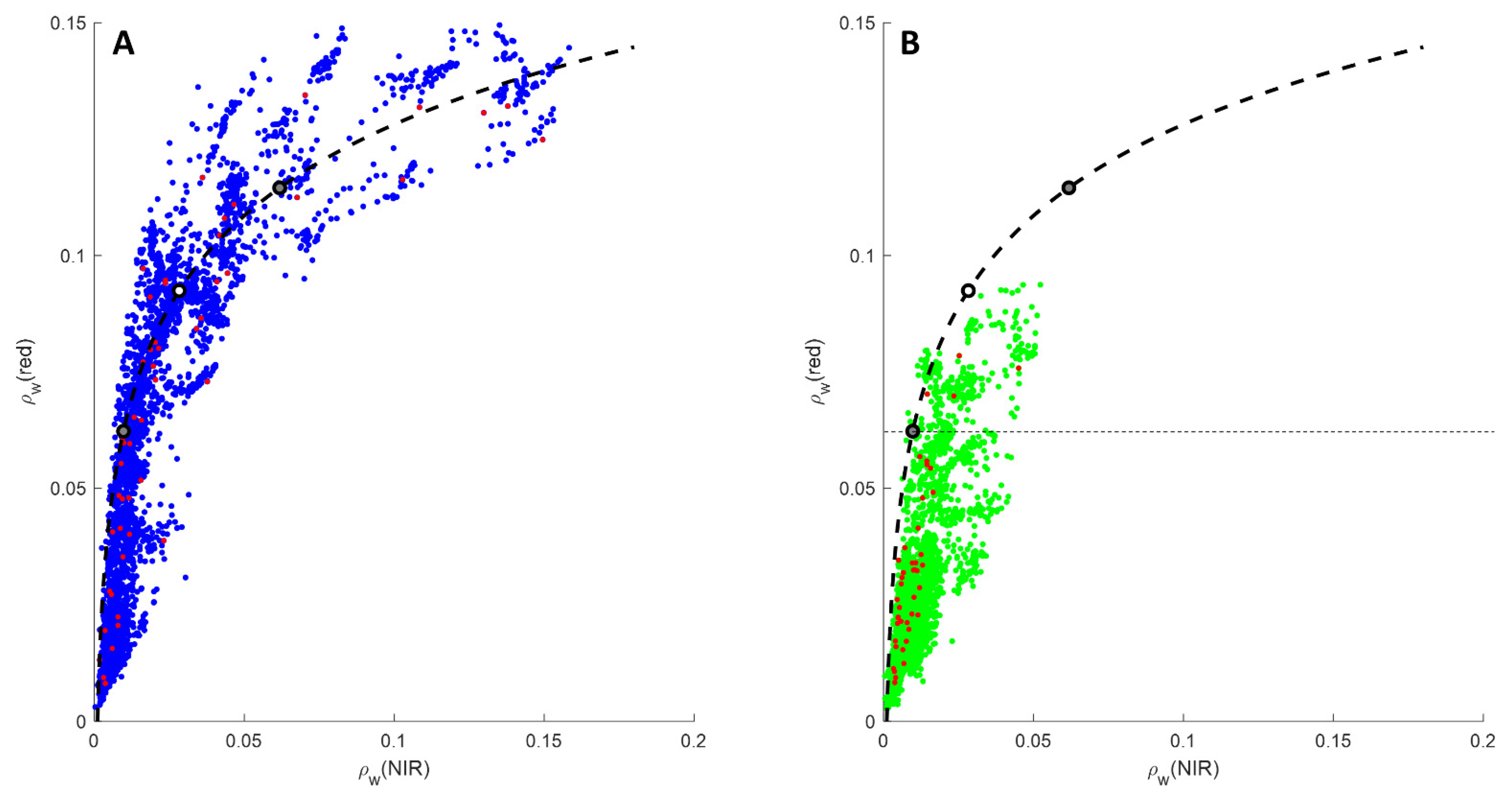
Appendix A.2. Computation of Switching Algorithm Radiometric Bounds


References
- Metzger, M.J.; Bunce, R.G.H.; Jongman, R.H.G.; Mücher, C.A.; Watkins, J.W. A Climatic Stratification of the Environment of Europe. Glob. Ecol. Biogeogr. 2005, 14, 549–563. [Google Scholar] [CrossRef]
- Kim, J.-S.; Seo, K.-W.; Jeon, T.; Chen, J.; Wilson, C.R. Missing Hydrological Contribution to Sea Level Rise. Geophys. Res. Lett. 2019, 46, 12049–12055. [Google Scholar] [CrossRef] [Green Version]
- Colmet-Daage, A.; Sanchez-Gomez, E.; Ricci, S.; Llovel, C.; Borrell Estupina, V.; Quintana-Seguí, P.; Llasat, M.C.; Servat, E. Evaluation of Uncertainties in Mean and Extreme Precipitation under Climate Change for Northwestern Mediterranean Watersheds from High-Resolution Med and Euro-CORDEX Ensembles. Hydrol. Earth Syst. Sci. 2018, 22, 673–687. [Google Scholar] [CrossRef] [Green Version]
- Martinez, J.M.; Guyot, J.L.; Filizola, N.; Sondag, F. Increase in Suspended Sediment Discharge of the Amazon River Assessed by Monitoring Network and Satellite Data. CATENA 2009, 79, 257–264. [Google Scholar] [CrossRef] [Green Version]
- Eisma, D.; Bernard, P.; Cadée, G.C.; Ittekkot, V.; Kalf, J.; Laane, R.; Martin, J.M.; Mook, W.G.; Van Put, A.; Schuhmacher, T. Suspended-Matter Particle Size in Some West-European Estuaries; Part I: Particle-Size Distribution. Neth. J. Sea Res. 1991, 28, 193–214. [Google Scholar] [CrossRef]
- Eisma, D.; Bernard, P.; Cadée, G.C.; Ittekkot, V.; Kalf, J.; Laane, R.; Martin, J.M.; Mook, W.G.; van Put, A.; Schuhmacher, T. Suspended-Matter Particle Size in Some West-European Estuaries; Part II: A Review on Floc Formation and Break-Up. Neth. J. Sea Res. 1991, 28, 215–220. [Google Scholar] [CrossRef]
- Kuprenas, R.; Tran, D.; Strom, K. A Shear-Limited Flocculation Model for Dynamically Predicting Average Floc Size. J. Geophys. Res. Ocean. 2018, 123, 6736–6752. [Google Scholar] [CrossRef]
- Eyrolle, F.; Lepage, H.; Antonelli, C.; Morereau, A.; Cossonnet, C.; Boyer, P.; Gurriaran, R. Radionuclides in Waters and Suspended Sediments in the Rhone River (France)-Current Contents, Anthropic Pressures and Trajectories. Sci. Total Environ. 2020, 723, 137873. [Google Scholar] [CrossRef]
- Jalón-Rojas, I.; Schmidt, S.; Sottolichio, A. Comparison of Environmental Forcings Affecting Suspended Sediments Variability in Two Macrotidal, Highly-Turbid Estuaries. Estuar. Coast. Shelf Sci. 2017, 198, 529–541. [Google Scholar] [CrossRef]
- Jalón-Rojas, I.; Sottolichio, A.; Hanquiez, V.; Fort, A.; Schmidt, S. To What Extent Multidecadal Changes in Morphology and Fluvial Discharge Impact Tide in a Convergent (Turbid) Tidal River. J. Geophys. Res. Ocean. 2018, 123, 3241–3258. [Google Scholar] [CrossRef]
- Lorthiois, T.; Doxaran, D.; Chami, M. Daily and Seasonal Dynamics of Suspended Particles in the Rhône River Plume Based on Remote Sensing and Field Optical Measurements. Geo-Mar. Lett. 2012, 32, 89–101. [Google Scholar] [CrossRef]
- Ody, A.; Doxaran, D.; Vanhellemont, Q.; Nechad, B.; Novoa, S.; Many, G.; Bourrin, F.; Verney, R.; Pairaud, I.; Gentili, B. Potential of High Spatial and Temporal Ocean Color Satellite Data to Study the Dynamics of Suspended Particles in a Micro-Tidal River Plume. Remote Sens. 2016, 8, 245. [Google Scholar] [CrossRef] [Green Version]
- Doxaran, D.; Froidefond, J.-M.; Castaing, P.; Babin, M. Dynamics of the Turbidity Maximum Zone in a Macrotidal Estuary (the Gironde, France): Observations from Field and MODIS Satellite Data. Estuar. Coast. Shelf Sci. 2009, 81, 321–332. [Google Scholar] [CrossRef]
- Novoa, S.; Doxaran, D.; Ody, A.; Vanhellemont, Q.; Lafon, V.; Lubac, B.; Gernez, P. Atmospheric Corrections and Multi-Conditional Algorithm for Multi-Sensor Remote Sensing of Suspended Particulate Matter in Low-to-High Turbidity Levels Coastal Waters. Remote Sens. 2017, 9, 61. [Google Scholar] [CrossRef] [Green Version]
- Gangloff, A.; Verney, R.; Doxaran, D.; Ody, A.; Estournel, C. Investigating Rhône River Plume (Gulf of Lions, France) Dynamics Using Metrics Analysis from the MERIS 300m Ocean Color Archive (2002−2012). Cont. Shelf Res. 2017, 144. [Google Scholar] [CrossRef] [Green Version]
- Durrieu De Madron, X.; Abassi, A.; Heussner, S.; Monaco, A.; Aloisi, J.C.; Radakovitch, O.; Giresse, P.; Buscail, R.; Kerherve, P. Particulate Matter and Organic Carbon Budgets for the Gulf of Lions (NW Mediterranean). Oceanol. Acta 2000, 23, 717–730. [Google Scholar] [CrossRef] [Green Version]
- Bourrin, F.; Durrieu de Madron, X. Contribution to the Study of Coastal Rivers and Associated Prodeltas to Sediment Supply in Gulf of Lions (N-W Mediterranean Sea). Vie Et Milieu 2006, 56, 1–8. [Google Scholar]
- Pont, D.; Simonnet, J.-P.; Walter, A.V. Medium-Term Changes in Suspended Sediment Delivery to the Ocean: Consequences of Catchment Heterogeneity and River Management (Rhône River, France). Estuar. Coast. Shelf Sci. 2002, 54, 1–18. [Google Scholar] [CrossRef]
- Broche, P.; Devenon, J.-L.; Forget, P.; de Maistre, J.-C.; Naudin, J.-J.; Cauwet, G. Experimental Study of the Rhone Plume. Part I: Physics and Dynamics. Oceanol. Acta 1998, 21, 725–738. [Google Scholar] [CrossRef] [Green Version]
- Estournel, C.; Kondrachoff, V.; Marsaleix, P.; Vehil, R. The Plume of the Rhone: Numerical Simulation and Remote Sensing. Cont. Shelf Res. 1997, 17, 899–924. [Google Scholar] [CrossRef]
- Estournel, C.; Broche, P.; Marsaleix, P.; Devenon, J.-L.; Auclair, F.; Vehil, R. The Rhone River Plume in Unsteady Conditions: Numerical and Experimental Results. Estuar. Coast. Shelf Sci. 2001, 53, 25–38. [Google Scholar] [CrossRef]
- Aloisi, J.; Cambon, J.; Carbonne, J.; Cauwet, G.; Millot, C.; Monaco, A.; Pauc, H. Origine et rôle du néphéloïde profond dans le transfert des particules au milieu marin. Application au Golfe du Lion. Oceanol. Acta 1982, 5, 481–491. [Google Scholar]
- Many, G.; Bourrin, F.; Durrieu de Madron, X.; Pairaud, I.; Gangloff, A.; Doxaran, D.; Ody, A.; Verney, R.; Menniti, C.; Le Berre, D.; et al. Particle Assemblage Characterization in the Rhone River ROFI. J. Mar. Syst. 2016, 157, 39–51. [Google Scholar] [CrossRef] [Green Version]
- Eyrolle, F.; Antonelli, C.; Raimbault, P.; Boullier, V.; Fornier, M.; Sivade, E. A High Frequency Flux Monitoring Station of Suspended Sediments, Nutrients and Pollutants at the Lower Rhône River (SORA). In Proceedings of the I.S. River Internayional Conference, Lyon, France, 25–28 June 2012; Available online: https://www.graie.org/ISRivers/actes/pdf2012/2C212-253EYR.pdf (accessed on 3 March 2022).
- Infrastructure de recherche littorale et côtière (ILICO). Available online: https://www.ir-ilico.fr (accessed on 28 February 2022).
- Poulier, G.; Launay, M.; Le Bescond, C.; Thollet, F.; Coquery, M.; Le Coz, J. Combining Flux Monitoring and Data Reconstruction to Establish Annual Budgets of Suspended Particulate Matter, Mercury and PCB in the Rhône River from Lake Geneva to the Mediterranean Sea. Sci. Total Environ. 2019, 658, 457–473. [Google Scholar] [CrossRef]
- Mobley, C.D. Estimation of the Remote-Sensing Reflectance from above-Surface Measurements. Appl. Opt. AO 1999, 38, 7442–7455. [Google Scholar] [CrossRef] [PubMed]
- Ruddick, K.G.; De Cauwer, V.; Park, Y.-J.; Moore, G. Seaborne Measurements of near Infrared Water-Leaving Reflectance: The Similarity Spectrum for Turbid Waters. Limnol. Oceanogr. 2006, 51, 1167–1179. [Google Scholar] [CrossRef] [Green Version]
- Aminot, A.; Kérouel, R. Hydrologie des Ecosystèmes Marins—Paramètres et Analyses; Methodes D’analyse en Milieu Marin; Ifremer Plouzane: Plouzané, France, 2004; Volume 29, ISBN 978-2-84433-133-5. [Google Scholar]
- Vanhellemont, Q.; Ruddick, K. Acolite for Sentinel-2: Aquatic Applications of Msi Imagery. In Proceedings of the 2016 ESA Living Planet Symposium, Prague, Czech Republic, 9–13 May 2016; p. 8. [Google Scholar]
- Vanhellemont, Q. Adaptation of the Dark Spectrum Fitting Atmospheric Correction for Aquatic Applications of the Landsat and Sentinel-2 Archives. Remote Sens. Environ. 2019, 225, 175–192. [Google Scholar] [CrossRef]
- Vanhellemont, Q.; Ruddick, K. Atmospheric Correction of Metre-Scale Optical Satellite Data for Inland and Coastal Water Applications. Remote Sens. Environ. 2018, 216, 586–597. [Google Scholar] [CrossRef]
- Harmel, T.; Chami, M.; Tormos, T.; Reynaud, N.; Danis, P.-A. Sunglint Correction of the Multi-Spectral Instrument (MSI)-SENTINEL-2 Imagery over Inland and Sea Waters from SWIR Bands. Remote Sens. Environ. 2018, 204, 308–321. [Google Scholar] [CrossRef]
- Ruddick, K.G.; Ovidio, F.; Rijkeboer, M. Atmospheric Correction of SeaWiFS Imagery for Turbid Coastal and Inland Waters. Appl. Opt. 2000, 39, 897. [Google Scholar] [CrossRef] [Green Version]
- Wang, M.; Tang, J.; Shi, W. MODIS-Derived Ocean Color Products along the China East Coastal Region. Geophys. Res. Lett. 2007, 34. [Google Scholar] [CrossRef]
- Shen, F.; Verhoef, W.; Zhou, Y.; Salama, M.S.; Liu, X. Satellite Estimates of Wide-Range Suspended Sediment Concentrations in Changjiang (Yangtze) Estuary Using MERIS Data. Estuaries Coasts 2010, 33, 1420–1429. [Google Scholar] [CrossRef]
- Knaeps, E.; Ruddick, K.G.; Doxaran, D.; Dogliotti, A.I.; Nechad, B.; Raymaekers, D.; Sterckx, S. A SWIR Based Algorithm to Retrieve Total Suspended Matter in Extremely Turbid Waters. Remote Sens. Environ. 2015, 168, 66–79. [Google Scholar] [CrossRef] [Green Version]
- Nechad, B.; Ruddick, K.G.; Park, Y. Calibration and Validation of a Generic Multisensor Algorithm for Mapping of Total Suspended Matter in Turbid Waters. Remote Sens. Environ. 2010, 114, 854–866. [Google Scholar] [CrossRef]
- Lorthiois, T. Dynamique Des Matières En Suspension Dans Le Panache Du Rhône (Méditerranée Occidentale) Par Télédétection Spatiale “Couleur de l’océan”. Ph.D. Thesis, Université Pierre et Marie Curie-Paris VI, Paris, France, 2012. [Google Scholar]
- Luo, Y.; Doxaran, D.; Ruddick, K.; Shen, F.; Gentili, B.; Yan, L.; Huang, H. Saturation of Water Reflectance in Extremely Turbid Media Based on Field Measurements, Satellite Data and Bio-Optical Modelling. Opt. Express OE 2018, 26, 10435–10451. [Google Scholar] [CrossRef] [PubMed] [Green Version]
- Sterckx, S.; Knaeps, S.; Kratzer, S.; Ruddick, K. SIMilarity Environment Correction (SIMEC) Applied to MERIS Data over Inland and Coastal Waters. Remote Sens. Environ. 2015, 157, 96–110. [Google Scholar] [CrossRef]
- Chan, T.F.; Vese, L.A. Active Contours without Edges. IEEE Trans. Image Processing 2001, 10, 266–277. [Google Scholar] [CrossRef] [Green Version]
- Luo, Y.; Doxaran, D.; Vanhellemont, Q. Retrieval and Validation of Water Turbidity at Metre-Scale Using Pléiades Satellite Data: A Case Study in the Gironde Estuary. Remote Sens. 2020, 12, 946. [Google Scholar] [CrossRef] [Green Version]
- Wójcik, K.A.; Bialik, R.J.; Osińska, M.; Figielski, M. Investigation of Sediment-Rich Glacial Meltwater Plumes Using a High-Resolution Multispectral Sensor Mounted on an Unmanned Aerial Vehicle. Water 2019, 11, 2405. [Google Scholar] [CrossRef] [Green Version]
- Sadaoui, M.; Ludwig, W.; Bourrin, F.; Raimbault, P. Controls, Budgets and Variability of Riverine Sediment Fluxes to the Gulf of Lions (NW Mediterranean Sea). J. Hydrol. 2016, 540, 1002–1015. [Google Scholar] [CrossRef]
- HORLER, D.N.H.; DOCKRAY, M.; BARBER, J. The Red Edge of Plant Leaf Reflectance. Int. J. Remote Sens. 1983, 4, 273–288. [Google Scholar] [CrossRef]
- Dogliotti, A.I.; Ruddick, K.G.; Nechad, B.; Doxaran, D.; Knaeps, E. A Single Algorithm to Retrieve Turbidity from Remotely-Sensed Data in All Coastal and Estuarine Waters. Remote Sens. Environ. 2015, 156, 157–168. [Google Scholar] [CrossRef] [Green Version]
- Tavora, J.; Boss, E.; Doxaran, D.; Hill, P. An Algorithm to Estimate Suspended Particulate Matter Concentrations and Associated Uncertainties from Remote Sensing Reflectance in Coastal Environments. Remote Sens. 2020, 12, 2172. [Google Scholar] [CrossRef]
- Ludwig, W.; Probst, J.-L.; Kempe, S. Predicting the Oceanic Input of Organic Carbon by Continental Erosion. Glob. Biogeochem. Cycles 1996, 10, 23–41. [Google Scholar] [CrossRef] [Green Version]
- Ludwig, W.; Dumont, E.; Meybeck, M.; Heussner, S. River Discharges of Water and Nutrients to the Mediterranean and Black Sea: Major Drivers for Ecosystem Changes during Past and Future Decades? Prog. Oceanogr. 2009, 80, 199–217. [Google Scholar] [CrossRef]
- Ludwig, W.; Bouwman, A.F.; Dumont, E.; Lespinas, F. Water and Nutrient Fluxes from Major Mediterranean and Black Sea Rivers: Past and Future Trends and Their Implications for the Basin Scale Budgets. Glob. Biogeochem. Cycles 2010, 24. [Google Scholar] [CrossRef]
- Schlünz, B.; Schneider, R. Transport of Terrestrial Organic Carbon to the Oceans by Rivers: Re-Estimating Flux- and Burial Rates. Int. J. Earth Sci. 2000, 88, 599–606. [Google Scholar] [CrossRef]
- Many, G.; Bourrin, F.; Durrieu de Madron, X.; Ody, A.; Doxaran, D.; Cauchy, P. Glider and Satellite Monitoring of the Variability of the Suspended Particle Distribution and Size in the Rhône ROFI. Prog. Oceanogr. 2018, 163, 123–135. [Google Scholar] [CrossRef] [Green Version]
- Pastor, F.; Valiente, J.A.; Palau, J.L. Sea Surface Temperature in the Mediterranean: Trends and Spatial Patterns (1982–2016). Pure Appl. Geophys. 2018, 175, 4017–4029. [Google Scholar] [CrossRef] [Green Version]
- Babin, M.; Stramski, D. Variations in the Mass-Specific Absorption Coefficient of Mineral Particles Suspended in Water. Limnol. Oceanogr. 2004, 49, 756–767. [Google Scholar] [CrossRef] [Green Version]
- Estapa, M.L.; Boss, E.; Mayer, L.; Roesler, C. Role of Iron and Organic Carbon in Mass-Specific Light Absorption by Particulate Matter from Louisiana Coastal Waters. Limnol. Oceanogr. 2012, 57, 97–112. [Google Scholar] [CrossRef] [Green Version]


| Sensor Bands | Location | Number of Fitted Data (N) | MSI | OLI | MODIS | |||||||||
|---|---|---|---|---|---|---|---|---|---|---|---|---|---|---|
| Aρ (g.m−3) | 95% | Cρ | R2 | Aρ (g.m−3) | 95% | Cρ | R2 | Aρ (g.m−3) | 95% | Cρ | R2 | |||
| Green | Rhône River plume | 21 (field campaigns) | 69 | 57;80 | 0.1449 | 0.60 | 76 | 66;86 | 0.1449 | 0.68 | 66 | 55;78 | 0.1449 | 0.56 |
| Red | Rhône River plume | 90 (field campaigns) | 228 | 212;244 | 0.1728 | 0.72 | 208 | 193;222 | 0.1686 | 0.71 | 193 | 179;206 | 0.1641 | 0.70 |
| NIR | Rhône River plume and SORA station | 89 (field campaigns) 38 (MSI vs. SORA) 32 (OLI vs. SORA) | 2738 | 2524;2952 | 0.1838 | 0.98 | 2743 | 2529;2958 | 0.1835 | 0.98 | 2572 | 2372;2773 | 0.1961 | 0.98 |
| ρw(R) Interval | Used SPM Concentration | Weighted Factors | |||||||||||||||||||||||||||
|---|---|---|---|---|---|---|---|---|---|---|---|---|---|---|---|---|---|---|---|---|---|---|---|---|---|---|---|---|---|
| <G2R | SPMG | α = 1 | β = 1 | γ = 0 | |||||||||||||||||||||||||
| [G2R; R2N] | Saturation interval: SPMG and SPMR | γ = 0 | |||||||||||||||||||||||||||
| [R2N; N] | Saturation interval: SPMR and SPMNIR | α = 0 | |||||||||||||||||||||||||||
| >N | SPMNIR | α = 0 | β = 0 | γ = 1 | |||||||||||||||||||||||||
| ρω(R) | G2R | SG | R2N | SR | N | ||||||||||||||||||||||||
| Sensors | |||||||||||||||||||||||||||||
| MSI | 0.0103 | 0.0301 | 0.0588 | 0.0879 | 0.11 | ||||||||||||||||||||||||
| OLI | 0.0102 | 0.0297 | 0.0622 | 0.0924 | 0.1145 | ||||||||||||||||||||||||
| MODIS | 0.0102 | 0.0298 | 0.0624 | 0.0936 | 0.117 | ||||||||||||||||||||||||
| X | y | Discharge Interval (m3.s−1) | A | B | R2 |
|---|---|---|---|---|---|
| River discharge (m3.s−1) | SPMS (g.m−3) | 300–3000 | 1.462 × 10−05 | 1.943 | 0.65 |
| River discharge (m3.s−1) | SPMS (g.m−3) | 3000–5500 | 2.236 × 10⁻¹⁴ | 4.46 | 0.41 |
| River discharge (m3.s−1) | SPMM (g.m−3) | 500–3000 | 1.795 × 10−05 | 1.777 | 0.70 |
| River discharge (m3.s−1) | SPMM (g.m−3) | 3000–4500 | 8.913 × 10⁻¹⁰ | 3.079 | 0.20 |
| River discharge (m3.s−1) | Plume mass (MLB; MUB) (t) | 500–5000 | 1.122 × 10⁻¹¹ (7.08 × 10⁻¹²;1.622 × 10⁻¹¹) | 4.167 (4.189; 4.182) | 0.66 (0.62; 0.68) |
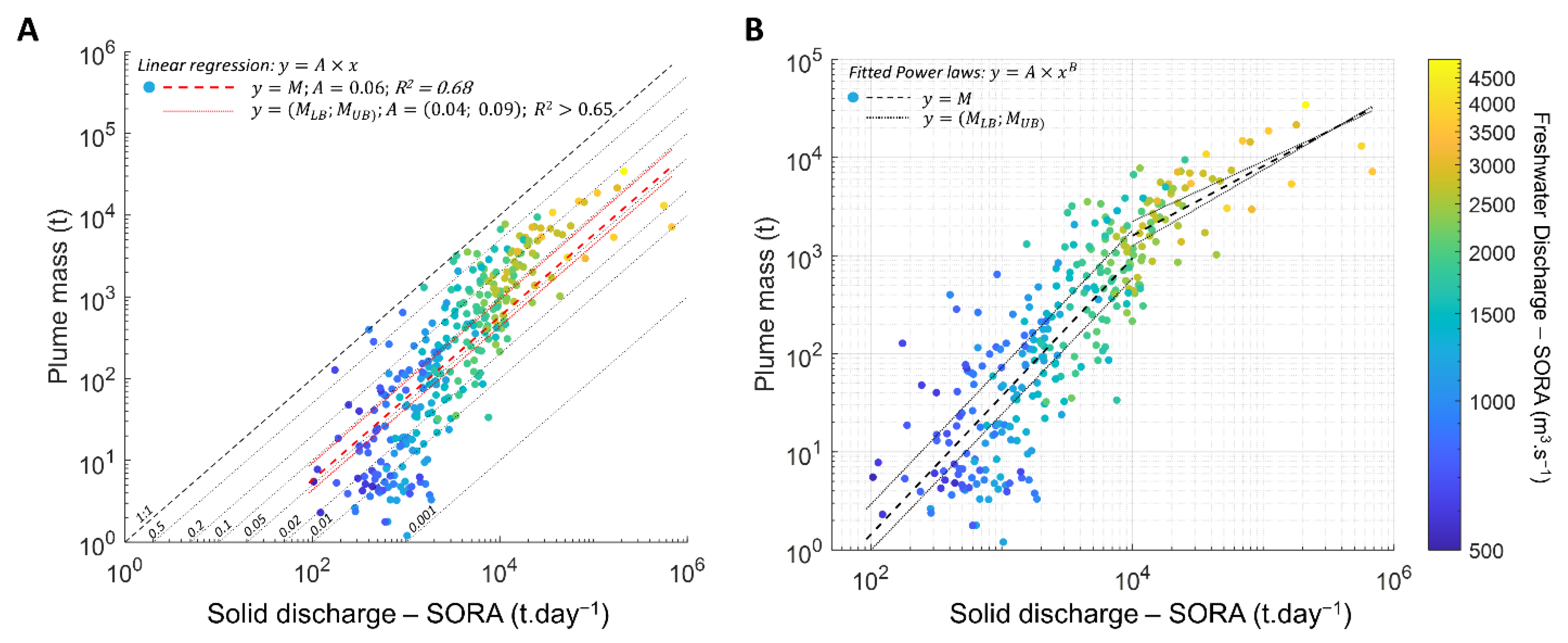
| Solid discharge (t.day−1) | Plume mass (MLB; MUB) (t) | 1–1 × 10⁴ | 0.0022 (0.0017; 0.0047) | 1.407 (1.383; 1.396) | 0.57 (0.50; 0.62) |
| Solid discharge (t.day−1) | Plume mass (MLB; MUB) (t) | 1–7 × 10⁵ | 2.319 (0.977; 7.849) | 0.71 (0.777; 0.613) | 0.4 (0.42; 0.25) |
| Linear regression: + B | |||||
| River discharge (m3.s−1) | Plume surface (SLB; SUB) (km2) | 500–5000 | 0.1824 (0.1366;0.2683) | −175.7 (−131.3; −210) | 0.57 (0.54; 0.40) |
| Solid discharge (t.day−1) | Plume mass (MLB; MUB) (t) | 1–7 × 10⁵ | 0.06 (0.04; 0.09) | - | 0.68 (0.65; 0.69) |
Publisher’s Note: MDPI stays neutral with regard to jurisdictional claims in published maps and institutional affiliations. |
© 2022 by the authors. Licensee MDPI, Basel, Switzerland. This article is an open access article distributed under the terms and conditions of the Creative Commons Attribution (CC BY) license (https://creativecommons.org/licenses/by/4.0/).
Share and Cite
Ody, A.; Doxaran, D.; Verney, R.; Bourrin, F.; Morin, G.P.; Pairaud, I.; Gangloff, A. Ocean Color Remote Sensing of Suspended Sediments along a Continuum from Rivers to River Plumes: Concentration, Transport, Fluxes and Dynamics. Remote Sens. 2022, 14, 2026. https://doi.org/10.3390/rs14092026
Ody A, Doxaran D, Verney R, Bourrin F, Morin GP, Pairaud I, Gangloff A. Ocean Color Remote Sensing of Suspended Sediments along a Continuum from Rivers to River Plumes: Concentration, Transport, Fluxes and Dynamics. Remote Sensing. 2022; 14(9):2026. https://doi.org/10.3390/rs14092026
Chicago/Turabian StyleOdy, Anouck, David Doxaran, Romaric Verney, François Bourrin, Guillaume P. Morin, Ivane Pairaud, and Aurélien Gangloff. 2022. "Ocean Color Remote Sensing of Suspended Sediments along a Continuum from Rivers to River Plumes: Concentration, Transport, Fluxes and Dynamics" Remote Sensing 14, no. 9: 2026. https://doi.org/10.3390/rs14092026