Simple Summary
Multi-satellite observations to jointly analyze extreme surface wind and wave properties can now be readily obtained to study tropical cyclone (TC) events. Developing over the Philippine Sea, TC Goni was one of the most powerful TCs in 2020. Constrained by Sentinel-1/RadarSat-2 SAR and CFOSAT SCAT satellite data, wind field in the intense TC region is reconstructed. Significant wave height measurements are further obtained from altimeters on-board the CFOSAT, Jason-3, and Sentinel-3A, B satellites. The directional wave spectrum information can be derived from the CFOSAT SWIM off-nadir radar measurements. Using a simplified 2D parametric model and derived self-similar analytical solutions, the measured surface wave amplification in the right-hand TC sector, relative to its propagation direction, is well captured and interpreted. For TC Goni, observed and predicted waves reach 8 m and wavelengths larger than 200 m, leaving the TC inner region in the forward and forward-left direction. In the far TC zone, swell attenuates and superposes with wind waves, not necessarily aligned, to give observed significant wave height values. Multi-satellite data together with simplified parametric model outputs open new perspectives to more precisely study and predict surface waves generated by moving and rapidly evolving TCs for different scientific and practical purposes.
Abstract
Over the Philippine Sea, the tropical cyclone (TC) Goni reaches category 5 on 29–31 October 2020. Multi-satellite observations, including CFOSAT SWIM/SCAT and Sentinel-1 SAR data, are jointly analyzed to assess the performances of a parametric model. Recently developed to provide a fast estimation of surface wave developments under rapidly evolving TCs, this full 2D parametric model (KYCM) and its simplified self-similar solutions (TC-wave geophysical model function (TCW GMF)) are thoroughly compared with satellite observations. TCW GMF provides immediate first-guess estimates, at any location in space and time, for the significant wave height, wavelength, and wave direction parameters. Moving cyclones trigger strong asymmetrical wave fields, associated to a resonance between wave group velocity and TC heading velocity. For TC Goni, this effect is well evidenced and captured, leading to extreme waves reaching up to 8 m, further outrunning as swell systems with wavelengths about 200–250 m in the TC heading direction, slightly shifted leftwards. Considering wind field constrained with very highly resolved Sentinel-1 SAR measurements and medium resolution CFOSAT SCAT data, quantitative agreements between satellite measurements and KYCM/TCW GMF results are obtained. Far from the TC inner core (∼10 radii of maximum wind speed), the superposition of outrunning swell systems and local wind waves estimates leads to Hs values very close to altimeter measurements. This case study demonstrates the promising capabilities to combine multi-satellite observations, with analytical self-similar solutions to advance improved understandings of surface wave generation under extreme wind conditions.
1. Introduction
Not only for marine engineering and navigation safety, hurricane-generated wind and wave fields are essential components of the two-way, air-ocean coupled system to enter the dynamical evolution of extreme events [1,2,3]. Still, the generation and evolution of surface waves in high-wind conditions and extreme fetches remain poorly understood. Rare and relatively small in size, these extreme systems are furthermore difficult to sample well with in situ measurements. Despite thorough continuous space-borne and in-field (buoys, airborne) monitoring [4,5,6,7,8], extreme weather events thus generally lack very precise information, especially regarding rapidly evolving wind fields, the associated local waves, and outrunning swell systems [9,10]. Vector wind fields over oceans are now routinely provided by scatterometer observations [11,12,13]. Yet, precise estimations of tropical cyclone (TC) intensity using scatterometer data remain challenging, due to moderate to low spatial resolution compared to TC structure, rain precipitations, and possible signal saturation in radar backscatter measurements, see e.g., [14].
For numerical simulations, TC generated wave fields have been developed for decades [15,16,17,18,19]. Surface wave models have then largely proved their overall reliability, but performances under extreme conditions remain limited. One of such studies, reported by [20] for TC Bonnie, demonstrated that WAVEWATCH III numerical model outputs can efficiently match scanning radar altimeter measurements inside the tropical cyclone region. This proves the model capability to reproduce the wave fields when the extreme wind conditions are correctly prescribed. However, precise knowledge of the space-time rapidly evolving surface wind field is not always available. Wind forcing uncertainties may then cause large biases for surface momentum fluxes and wave developments. This may likely be a reason for swell, generated by strong storms, to be poorly predicted by forecast models, both in magnitude and arrival time [21].
To help estimate space-time varying wind conditions and possibly consider ensembles of solutions, more simplified solutions were developed and presented by [22,23]. The proposed two-dimensional parametric model readily provides the main statistical characteristics of surface waves. Performing numerical experiments, simplified self-similar solutions, termed TC-wave Geophysical Model Function (TCW GMF), were further derived to obtain first-guess estimates for arbitrary TC vortex shapes, defined by maximum wind speed , associated radius , and translation velocity V. Model and simplified TCW GMF solutions were already tested on documented in-field and satellite measurements. Particularly, the well-known wave intensification in the forward/right TC sector, relatively to the heading, resulting from a resonance between wave group velocity and TC heading velocity (e.g., [24,25,26,27,28]), was reproduced.
Augmenting the existing satellite capabilities to monitor extreme events, the satellite mission CFOSAT (China France Oceanography Satellite), launched in 2018, can now simultaneously provide ocean surface wind field and two-dimensional wave spectral distributions. CFOSAT indeed carries SCAT, a wind-field Ku-band scatterometer, and a unique real-aperture scanning radar system SWIM (Surface Waves Investigation and Monitoring), dedicated to ocean surface wave directional detection [29,30].
These new observations motivate the present work, to further assess the capabilities to jointly use the simplified model results and satellite observations.
A case of super typhoon Goni developing over the Philippine Sea on 29 October 2020 was selected for this study. As one of the strongest TCs ever recorded by one-minute average wind speed, Goni made landfall in the Philippines on November 1 with sustained winds of 195 mph and a central pressure of 884 mb, according to the Joint Typhoon Warning Center (JTWC). Strong winds associated with this TC damaged high-risk structures, houses, and some banana, rice, corn, and coconut plantations. A devastating storm surge of 3–6 m was predicted for a large swath of the coast and also caused catastrophic damage. Notice that the Japan Meteorological Agency’s wind speed estimate for Goni predicted 155 mph one-minute average winds, which strongly underestimates JTWC’s analysis, which was 195 mph. The latter relied on-satellite estimates, also using synthetic aperture radar (SAR) acquisition on 30 October, showing 180–185 mph winds at that time, matching Goni’s increasing intensity.
In the absence of the direct in-field measurements, satellite observations remain the most powerful and reliable for extreme winds/waves monitoring and forecasting, taking advantage of satellite data accessibility, regularity, wide swath, and now improved spatial resolution. To this end, the case of hurricane Goni corresponds to quasi-synchronously overlapping measurements from CFOSAT SWIM/SCAT and Sentinel-1 SAR measurements. For this case, very accurate and high resolution wind information is thus available to help compare wave model outputs and two-dimensional wave information. The analysis further benefits from other available satellite data, e.g., altimeters crossing TC Goni at different stages.
2. Satellite Data and Wave Modeling
TC Goni was the second most intense cyclone in 2020. Starting to intensify over the Philippine Sea on 29 October, TC Goni became a category 5 super typhoon on October 30th, with maximum wind speeds up to 85 m/s. TC Goni’s track is shown in Figure 1a, where color indicates the maximum wind speed. Within the TC region (±600 km from the TC center), altimeter measurements of significant wave height (Hs) from different satellites, CFOSAT, Jason-3, AltiKa, Sentinel-3A, and Sentinel-3B, can be gathered. Over the TC intensification region, enlarged on subplot Figure 1b, only altimeter few tracks are kept. TC standard parameters, maximum wind speed , radius of maximum wind speed , and translation speed V from the Best Track Data [31] are given in Figure 1c.
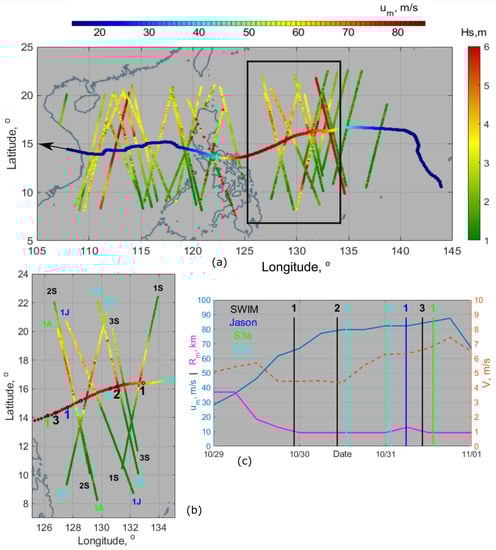
Figure 1.
(a) TC Goni track and altimeter measurements of Hs. (b) A fragment at the stage of TC intensification. Letters and colors indicate the altimeter names (CFOSAT, Jason-3, Sentinel-3A,B) and relative TC positions. (c) Time evolution of Goni parameters at its most intense stage.
2.1. TC Goni Surface Wind Information
At its peak intensity, the TC Goni wind field information can be obtained from observations acquired by synthetic aperture radars (SARs) on-board Sentinel-1A and RadarSat-2 and from CFOSAT SCAT scatterometer. Thanks to a dedicated strategy applied during the Satellite Hurricane Observation Campaign, SAR acquisitions are now more regularly tasked to provide wide swath observations in dual-polarization mode [32,33]. Based on these acquisitions, more accurate estimates of the ocean surface wind speed and direction can be obtained. For SAR acquisitions, this capability essentially relies on the use of the high wind sensitivity of measured cross-polarized signals [34]. Reference [35] fully demonstrated such a unique potential for estimating the TC parameters, especially the radius of maximum wind, . Combined with the co-polarized signals, the methodology also builds on wind streaks detected orientation [36] and TC center detection to apply a parametric inflow model using the formulation proposed by [37]. This algorithm, applied to each SAR scene, then provides a means to estimate the wind direction at the same resolution as the wind speed [33].
The CFOSAT SCAT is the Ku-band scatterometer with a rotating fan-beam dual-polarization radar with incidence angles within 28–51 (e.g., see the performance analysis in [38]). In the present work, the scatterometer data were processed by KNMI CFOSAT Wind Processor (CWDP) [39] deployed in the IFREMER Wave and Wind Operational Center computational facilities. The wind vector retrieval was done using NSCAT-4 Geophysical Modulation Function [13,40] together with ocean calibration correction [12] estimated over the sixty-day period around the targeted TC event. The standard 2DVAR algorithm [11,41] was applied to reduce wind vector ambiguities due to high wind speed gradients and precipitation impacts typically observed in zones of tropical storms.
On October 29th, tracks of Sentinel-1A and CFOSAT closely crossed the TC Goni eye within less than two hours, at 20:57 to 22:11, respectively. These two operating instruments complement each other. SAR data are fine-resolved on a swath of hundreds of km, and CFOSAT SCAT covers a ∼1000 km swath but at medium 25 km resolution. For TC Goni, is of the order of 10 km. Thus, not only considering precipitations possibly affecting the Ku-band CFOSAT SCAT measurements, the CFOSAT SCAT resolution is too coarse to provide accurate wind information in the wave-generation region. Note, C-band measurements are much less impacted by heavy precipitations. Furthermore, high resolution C-band SAR data can be more robustly filtered. Hence, SAR-derived wind field with resolution about 1 km can be derived, including the TC intense vortex region of maximum winds. Close in time and location, overlapping SAR and CFOSAT wind field fragments can further be merged, giving the priority to the high-resolution SAR data, using interpolation into a regular 1 km grid (Figure 2a). This data-driven wind field will then be considered to input the 2D parametric model. A comparison between wind speed radial distributions from SCAT and SAR data (Figure 2b) exhibits a clear agreement for TC radius larger than about 70 km. Closer to the TC center, SCAT-derived maximum wind speed is apparently underestimated compared to Best Track and SAR estimates.
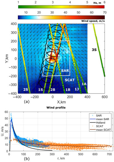
Figure 2.
(a) Merged Sentinel-1A SAR and CFOSAT SCAT wind data, altimeter estimates of Hs in TC reference system, and CFOSAT SWIM track for 10-inclined beam (black). (b) Wind speed radial distributions.
For other dates, either scatterometer or SAR data crossing TC Goni along its path could solely be used, supplemented with information from the Best Track Data.
Although the wind fields are generally asymmetric, a first guess can still be approximated using the Holland model [42], especially within the most intensified wind region, with axisymmetric wind speed with direction inwardly deviated from the tangential one by 20:
where is the Coriolis frequency (rad/s) with T the rotation period of the Earth (s) and the latitude, B the shape parameter ranging from about 0.7 to 2.5, and r the distance from the TC center (m); maximum wind speed and respective radius are measured here in m/s and m, correspondingly. This wind model is constrained using Best Track parameters and possible outer-core medium resolution scatterometer or radiometer measurements [43]. These practical first-guess wind fields can then feed the wave model simulations using the self-similar solutions (TCW GMF) [23].
For 29 October, fitting the SAR-derived wind profile with relation (1) gives = 15 km, = 47 m/s, B = 1.9 (the black line in Figure 2b). Note that the fitted maximum wind speed differs from the Best Track estimate (65 m/s). To model surface wave development, waves at a given location are not directly linked to the local wind but depend on the wind forcing effect integrated along the trajectory of the developing wave train. A typical spatial scale of wave development is of the order of the TC radius [23,44].
2.2. TC Goni Surface Waves
2.2.1. Data
Significant wave heights, wavelengths, and wave directions can all mostly be derived from the CFOSAT SWIM measurement. The SWIM instrument is a Ku-band radar with nadir and near-nadir scanning beam geometry designed to measure the spectral properties of surface ocean waves [29]. Directional wave spectra are recovered from scanning radar measurements, obtained by rotating beams pointing at 6, 8, and 10 mean incidence angles. On ground, a chosen beam will display a cycloid-like pattern, Figure 2a, for the 10 incidence. SWIM nadir products include Hs and the normalized radar cross-section interpreted in terms of surface wind speed, with accuracy similar to standard altimeter missions [45]. Other altimeter data come from satellites Jason-3, Sentinel-3A,B, and AltiKa. The latter was further excluded, with spurious strong Hs overestimation over the TC region, likely due to the strong sensitivity of Ka-band radar measurements to heavy precipitations. Over the cyclone intensification stage, 29–31 October, altimeter data were selected to cross the TC track at a distance not exceeding 600 km from the TC center. All these observations in the cyclone reference system are shown in Figure 2a.
2.2.2. Model Approach
Satellite data were analyzed together with the results of wave simulations using a recently developed 2D parametric model of the surface wave generation/evolution in the wind field varying in space and time [22].
Following [23], for TC conditions, full 2D parametric model calculations can be reduced to self-similar solutions, termed TCW GMF. These direct solutions are used to provide first-guess estimates of the wave field within the inner TC area, where the local inverse wave age exceeds a fixed value, taken equal to 0.6 in this study. The wind field prescribed by (1) with given values of , , B, and V is considered as the model input for TCW GMF. In the TC far zone, outside the contour , the self-similar solutions can be supplemented with analytical solutions of the parametric model equations, describing waves outrunning from the TC most intense area and propagating as swell systems.
The 2D parametric model equations and self-similar solutions for wind waves generated inside TC are recalled in Appendix A.1 and Appendix A.2, correspondingly. The simplified analytical solution for the outrunning swell systems, consistently linked with self-similar solutions valid within the TC intense region, are given in Appendix A.3. Hereinafter, we simply term the full 2D parametric model “KYCM” (Kudryavtsev–Yurovskaya–Chapron Model [22]) and its simplified version, combining TCW GMF and swell description, “TCW GMF”.
A flow chart to illustrate the procedure of joint analysis of satellite data and wave simulations is presented in Figure 3. Either KYMC or TCW GMF can by applied depending on the availability and quality of wind observations. If the wind field can be precisely reconstructed from satellite measurements over the whole considered area, it can be directly taken as model input in KYCM. Otherwise, the wind field prescribed by a Holland function (1) with , , and B taken from the Best Track Data or fitted using satellite measurements, is used as model input in TCW GMF (and can be used in KYCM as well). Another model input parameter, TC translation velocity, is always taken from the Best Track Data. The fields of wave height, wave length, and wave directions, both for wind waves and swell, are the model output.
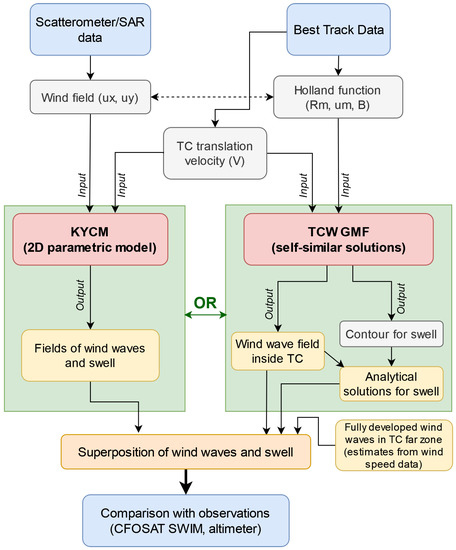
Figure 3.
A scheme illustrating joint analysis of satellite data and wave simulations, either KYCM or TCW GMF.
Far zone swell systems superimpose on “locally” generated wind waves, forming mixed sea conditions. For the sake of simplicity, we can assume that, in these regions, these local wind waves are nearly or fully developed, i.e., their energy directly related to the local wind speed. Using the Pierson–Moskovitz [46] expression, local Hs follows:
where is wind speed at 10 m level above the sea surface and g is gravity.
The mixed sea conditions in the TC far zone can thus be directly obtained to provide fast quantitative evaluations of TC generated wave fields, using (2) together with self-similar solutions within the TC inner intense zone and associated swell systems (TCW GMF). Alternatively, TC generated waves can also be obtained after numerical simulations using the full-2D parametric model (KYCM), Figure 3.
While the result of direct model calculations (KYCM) is more accurate, TCW GMF gives immediate first-guess estimates of wave fields in the cases when wind field information is insufficient to effectively use KYCM. The computational time of KYCM simulations is of the order of several minutes, depending on spatial resolution, swath, and forecast period (in our study, the forecast period is usually 48 h).
3. Results
3.1. TC Inner Core Region: Significant Wave Height and Wavelength Distribution
Firstly, the largest waves generated by the TC were estimated using the self-similar functions, Equations (A3) and (A4). The parameters = 15 km, = 47 m/s, and V = 5 m/s give = 5, corresponding to a “slow” TC (see Appendix A.2), leading to maximum wave height of 8.9 m and wavelength of 192 m. The Hs estimate is consistent with SWIM nadir-derived Hs (about 8 m). The peak wavelength derived from off-nadir SWIM measurements (not shown) is about 200 m, which is also in agreement with this first guess estimate.
The spatial distribution of significant wave height and wavelength of the longest waves, from numerical solution KYCM, driven by the wind field shown in Figure 2a and a TC translation velocity of 5 m/s, is presented in Figure 4a,b. The largest waves are predicted in the right TC sector (relative to the heading) to trace the expected wave group velocity resonance. This effect is well captured in all altimeter data from 29 to 31 October, including tracks passing hundreds of kilometers away from the TC center, either ahead of or behind it, i.e., the Hs colormap distribution on Figure 1b, comparing southern and northern regions relative to the TC track. For the considered case study, 29 October, Figure 4a,b, the maximum waves are predicted to turn left, somehow following the wind direction, and then leave the TC intense region through the front and front-left sector, becoming 200 m swell systems.
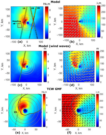
Figure 4.
KYMC−derived fields of and wavelength of (a,b) the longest waves among all waves and (c,d) the longest waves among pure wind waves. (e,f) Hs and wavelength fields from TCW GMF. A gray contour divides wind waves and swell regime. Colored circles are altimeter measurements.
Besides these primary wave systems, the KYCM also provides a method to possibly estimate, at any location, local shorter wave systems. Figure 4c,d shows the interpolation of wave rays corresponding to pure wind waves (inverse wave age greater than 0.85). The fields of the longest waves and pure wind waves coincide around the TC center and in the right (northern) TC sector. Over these regions, the wave field can be termed uni-modal. In the forward (western) and left (southern) sector, this is not the case. The wind waves and swell systems differ in both magnitude and direction. The two wave systems are clearly distinguished in Figure 5, corresponding to a fragment of the wave field, marked by the red square in Figure 4a. Figure 5a shows all wave rays in the TC reference frame, crossing the selected area during the entire calculation time (48 h). The average wavelength, wave height, and wave direction along each ray fragment is plotted in coordinates in Figure 5b. This provides wave evolution and angular spectral properties of the wave field inside the considered fragment. In particular, over this local region, it is expected that the two wave systems are almost following perpendicular propagation paths: the wind waves with wavelengths from several meters to 100 m, corresponding to different stages of their development, and respective Hs up to 3 m, are crossing a 200 m swell system with Hs about 4–5 m.
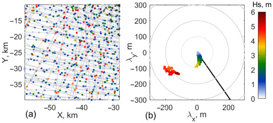
Figure 5.
(a) Wave ray-trains inside square area in Figure 4a. (b) Distribution of Hs; one point is one ray-averaged characteristic. Black line is wind direction.
The wave field distribution, combining TCW GMF results (Appendix A.2), with input parameters = 15 km, = 47 m/s, V = 5 m/s, and simplified swell solutions (Appendix A.3), appears very similar to the wave field derived from the numerical solutions of the KYCM, Figure 4e,f. “Pure” wind waves and swell at initial stage, predicted by TCW GMF, are confined within the region, delineated by the gray contour in Figure 4e,f. Beyond this boundary, the local degree of wave development, the inverse wave age , is below the value of 0.6. Wave trains crossing this contour start to follow a swell regime, with parameters (energy and wave length) calculated according to (A7) and (A8).
Altimeter measured Hs is shown in Figure 4 using colored circles as symbols. Figure 4a,e demonstrates that both full numerical simulation and TCW GMF quantitatively match, which is observed in the along-track SWIM altimeter Hs measurements (1S).
In more detail, along-track profiles of altimeter- and model-derived Hs for track 1S are compared on Figure 6a. Close to the TC center, the KYCM (green), TCW GMF (black), and altimeter data (blue) indicate that maximum waves reach Hs∼8 m. At km, TCW GMF-derived solutions, corresponding to pure swell systems, are apparently underestimated. Local wind waves, not accounted in this approach, explain such discrepancies. Indeed, in this sector, up to 200 km from the TC center, the wind remains strong, at about 20 m/s (see Figure 2a), to force energetic local wind waves. Moreover, traveling in high wind conditions, the inner-core generated waves turn to swell systems at a later stage than predicted by the Holland-based TCW GMF, evidenced with the green and black lines at Y∼100–200 km. Beyond this intermediate region, in the very far zone (∼400 km), swell systems again dominate, as confirmed with both KYCM and TCW GMF predictions.
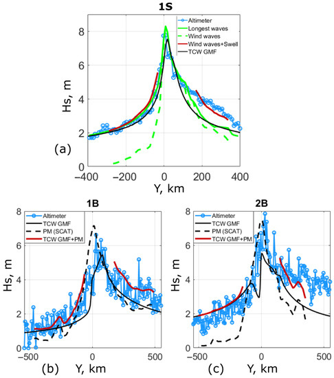
Figure 6.
Hs profiles along altimeter tracks 1S (a), 1B (b), 2B (c).
The superposition of the longest waves including swell systems (green solid line) and the longest pure wind waves (green dashed line) is shown with dark red. The two wave systems are distinguished with the estimated inverse wave age of the longest waves, larger or smaller than 0.85. Beyond this transition location, the longest waves will propagate without changing their directions. Hence, their wavenumber vector will start to deviate from the local wind direction. These swell waves are superimposed on other local systems of wind-generated waves (see Figure 4b,d as an example). A direct sum of the swell and wind-waves energy provides Hs level, coinciding with measurements. In the left TC sector (relative to the heading, ), far from the TC eye, wind waves are negligibly smaller than the swell generated by the TC. Over this region, the TCW GMF prediction is thus close to the KYCM result.
Sentinel-3 tracks 1B and 2B were also close to the TC Goni center but slightly behind and half/one day later. Altimeter data is quite scattered behind the TC, apparently due to precipitations, which can prevent precise determination of Ku-band measurements. As detected, [47,48], local heavy precipitations can indeed lead to poor performance of altimeter retrieval algorithms. At the time acquisitions of these measurements, the wind field changed, see Figure 1c. Still, this wind field evolution cannot entirely explain differences between modeled and observed Hs in the region that is east from the TC center, Figure 4a. Wind fields from both Sentinel-1 and RadarSat-2 data, closer in time, were then considered. Only slight differences in predicted Hs are obtained (not shown). A reason for this inconsistency can possibly be attributed to inaccurate wind directions, retrieved from the SAR data. In the area around the TC center, wind directions are indeed crucial to model wave development in the backward sector. Another reason can also arise from the possibly very complicated structure of the wave field behind the TC center. It is indeed regularly observed [8] and it will also be shown below for this TC that wave spectra in a TC backward area can display complex distributions.
Alternatively, TCW GMF estimates were augmented with underlying wind wave estimates to compare Hs transects along Sentinel-3 tracks 1B and 2B. The wind field follows the Holland function defined with Best Track Data parameters interpolated to the time of acquisition, with a decreased by about 5 m/s. Parameter B in Holland function (1) is further determined by approximating the wind profile using four parameters of the Best Track Data: and radii corresponding to 34, 50, and 64 kn. Resulting Hs profiles are shown Figure 6b,c. The overall Hs evolution is similar to the observed one and also the prediction using the KYCM driven by the SAR derived wind field (not shown). The Hs is underestimated around the TC center and north of it, especially for the track 2B. In the far zone, the local wind waves must be taken into account and superimposed to the generated swell systems. The wind wave contribution is shown with dashed lines and the superposition with the swell contribution with the dark-red line. Far from the TC center, the predicted wind wave contributions have similar profiles, either from the KYCM with wind field combining SAR and CFOSAT SCAT estimates or simply considering (2) with the local scatterometer-derived wind estimates (note that SAR coverage is only limited around the TC center).
All three considered cases demonstrate a good correspondence between predicted and measured Hs, with correlation coefficients equal to 0.94, 0.87, and 0.85, root mean square errors 0.4, 0.7, and 0.3, and biases −0.4, −0.4, and 0.1 for altimeter tracks 1S, 1B, and 2B, respectively.
3.2. Surface Wave Spectral Information
Besides Hs nadir measurements, the CFOSAT SWIM instrument uniquely provides wave spectral information [29]. The area covered by SWIM off-nadir measurements (colored circles on Figure 7a) is determined by the given inclination of a considered radar beam. Considering the whole rotation cycle, a full two-dimensional spectrum can be derived, corresponding to averaged spectral information over areas from tens to more than hundreds of km, again depending on the incidence angle. This resolution is seemingly too coarse to analyze waves, varying rapidly inside an intense TC region.
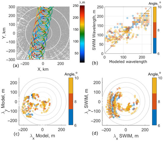
Figure 7.
(a) The modeled wave-rays (gray) and SWIM off-nadir measurements (6, 8 and 10 incidence angles). Color indicates the peak wavelength of 1D spectrum transect. (b) SWIM- and KYCM-derived wavelength comparison. (c) Wavelengths of modeled waves traveling in SWIM viewing direction in the vicinity of acquisition (9 km × 9 km). (d) Peak wavelengths of SWIM-derived spectrum transects.
Yet, spectral analysis over given transects can be considered independently to obtain wave spectral information more locally and at finer scales. This analysis is performed for each of the different SWIM beams, acquired on 29 October (1S). Modeled wave-trains inside 9 km × 9 km areas, with centers matching a given SWIM beam measurement, are considered. Average wavelengths and wave directions along wave rays are first plotted in (, ) coordinates; see an example in Figure 5. Only the wave-train with the largest wavelength is further taken into account. This wavelength is then compared with the peak wavelength determined from SWIM-transect 1D spectra. Data are then only kept when this direction is close to SWIM viewing azimuth (±15, accounting for 180 ambiguity). Points satisfying this condition are shown in Figure 7c,d for KYCM and SWIM, respectively.
For most cases, also corresponding to the longest waves, SWIM measurements indicate a preponderant west-south-west traveling direction, i.e., slightly leftwards of the TC heading direction. Wind wave systems with shorter wavelengths are detected to travel almost perpendicular to the TC heading direction. These distributions confirm the wavelength and wave direction fields predicted by KYCM, Figure 4b,d. A one-to-one wavelength comparison is presented in Figure 7b. Modeled and measured wavelengths generally agree, though large scatter is obtained. Part of it can presumably be attributed to noisy SWIM measurements, see Figure 7a. Still, the correlation coefficients for the different SWIM beams, 6, 8, and 10 incidence angles, are 0.73, 0.79, and 0.8, respectively. These beams are generally favored to derive wave spectral information [45]. However, wavelength distributions from two other SWIM radar beams, 2 and 4 incidence angles, are also found to be consistent with KYCM predictions. They clearly reveal the two groups of points: waves ∼150 m to the west (the northern part of SWIM track) and waves ∼200 m to the south-west (the southern part of SWIM track), Figure 8a,b; see also Figure 4b. The correlation coefficients for modeled and measured wavelengths, Figure 8c, are also high, at 0.78 and 0.71, respectively.
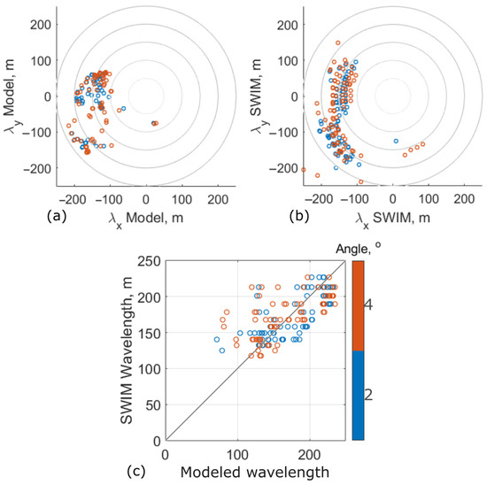
Figure 8.
Modeled and observed wavelength comparison for 2 and 4 SWIM beams. (a) Wavelengths of modeled waves traveling in SWIM viewing direction in the vicinity of acquisition. (b) Peak wavelengths of SWIM-derived spectrum transects. (c) SWIM- and KYCM-derived wavelength comparison.
The directional distribution of wavelengths within different TC sectors is presented on Figure 9. Notations on the left subplots are identical to Figure 7 a, but only small areas are considered. The middle subplots show SWIM-derived spectrum transects according to beam viewing azimuth. These spectra quite reliably provide information on wave peak location. The right subplots are modeled Hs distributions, which are described above (Figure 5). Though the comparison is indirect, KYCM predictions and SWIM data reveal strong similarities: wave systems intensify in the right and forward TC sectors (Figure 9a–f). For both, maximum wavelengths are about 200 m, and waves propagate slightly to the left relative to the TC heading. In the back TC sector, waves are less intensified, with wider directional distribution (Figure 9g–i). In the left-forward far zone, ∼300 km from the TC center, a 200 m south-west swell system dominates, Figure 9j–l. Generally, we can note quantitative agreements between observations and KYCM predictions for both peak wavelengths and directions.
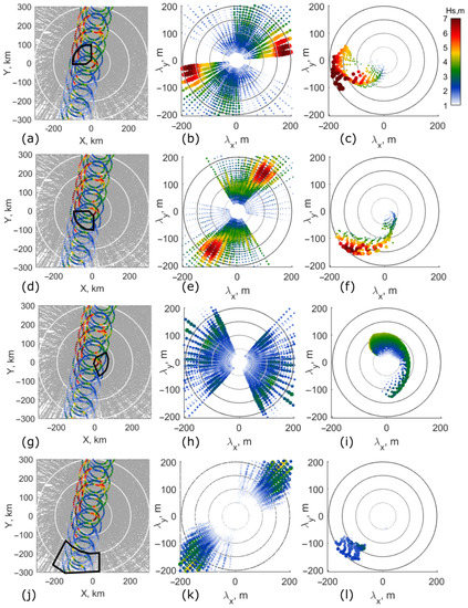
Figure 9.
Left column: the modeled wave-rays (gray), CFOSAT SWIM measurements (color indicates wave height of 1D spectrum peak), and considered TC areas (black contours). Middle column: SWIM-derived spectra transects inside a taken area; right column: Hs distributions of modeled waves.
3.3. TC Far Zone
Altimeter measurements 2S, 3S, 1J, and 1A are quite far from the TC center, Figure 2a. The local wind waves are expected to dominate the wave energy. For track 3S, the KYCM wave field using CFOSAT SCAT-derived wind field, Figure 10a, is shown in Figure 10b,c. For KYCM simulations, demonstrating fetch development, the wind input only corresponds to a fragment of the total wind field. Therefore, obvious artifacts are caused by an artificial wind field cutoff from the windward side. For such a case, only wave parameters far enough from this windward boundary, i.e., at a distance about 200 km, can be considered reliable.
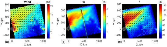
Figure 10.
Result of KYCM calculation with CFOSAT SCAT-derived wind input (track 3S). (a) The wind field; (b) Hs; (c) wavelength.
Along-track Hs profiles for this case, and also cases 2S, 1J, and 1A, derived from the KYCM with CFOSAT SCAT-derived wind field (the closest in time), are shown in Figure 11a–d with a green line. For comparison, the Pierson-Moskovits Hs, Equation (2), is also plotted (black-dashed line), corresponding to the upper limit of wind waves. First-guess estimates for the wavelength and direction of these wind waves considering the inverse wave age equal to 0.83 [46] and aligned with the wind direction are plotted with dashed lines in middle and bottom subplots. Comparing the KYCM results of Hs Figure 11a–d, wavelength Figure 11e–h, and wave direction Figure 11i–l, we can conclude that wind waves in the far zone are indeed close to fully developed conditions and propagate almost opposite to swell, Figure 11i–l.
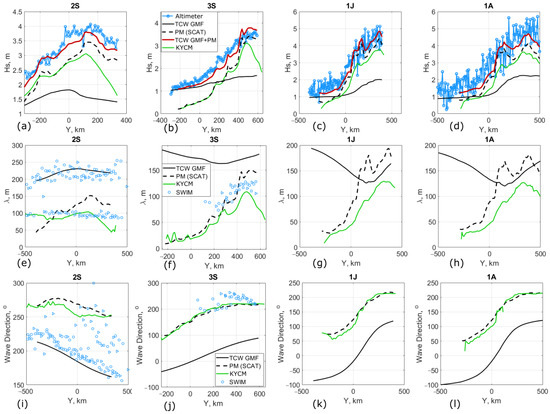
Figure 11.
Hs, wavelength and wave direction profiles in the far TC zone (altimeter tracks 2S, 3S, 1J, and 1A). (a) Hs, 2S; (b) Hs, 3S; (c) Hs, 1J; (d) Hs, 1A; (e) wavelength, 2S; (f) wavelength, 3S; (g) wavelength, 1J; (h) wavelength, 1A; (i) wave direction, 2S; (j) wave direction, 3S; (k) wave direction, 1J; (l) wave direction, 1A.
Again, the differences for the Hs and wavelength predictions, revealed at large Y, are artifacts caused by windward clipped wind field inputs. Thus, the use of Equation (2) can serve as an alternative and robust way to rapidly assess wind waves characteristics far from the TC center. Accounting for swell contributions is then important to bring our predictions in line with observations. In particular, in the far southern zone, the wind is low (see Figure 2a), and Hs of emerging swell from the TC center region is of the same order of magnitude or larger, Figure 9a–d. The superposition of wind waves, given by (2), and swell, given by TCW GMF (A7) and (A8), is shown with a dark-red line. It is highly correlated with altimeter-derived Hs; correlation coefficients are 0.93, 0.97, 0.94, and 0.88, root mean square errors 0.1, 0.1 0.25, and 0.53, and biases −0.2, −0.1, −0.1, and −0.4 for tracks 2S, 3S, 1J, and 1A, respectively.
For SWIM-off nadir measurements, Figure 12 presents a fragment of a time sequence of unidirectional modulation spectra for the radar beam. Respective wavelengths and wave directions for SWIM tracks 2S and 3S are shown with blue circles in Figure 11e,f,i,j. For the case of 3S, the radar spectra are very noisy to retrieve peak locations and only a part of the whole sequence can be considered. Still, it can reveal wind waves whose radar modulation amplitudes are larger than swell ones, Figure 11b,f,j. For 2S, swell is well distinguished, while wind waves are blurred, Figure 12. Secondary peaks can still be determined, close to wavenumbers corresponding to modeled wind waves, Figure 11e. KYCM/TCW GMF predictions and SWIM-derived wavelengths and directions are thus again in good agreement.
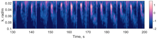
Figure 12.
Spectrum of CFOSAT SWIM radar signal modulations (divided by a wavenumber), shown in logarithmic color scale. A time sequence for inclined beam, track 2S.
4. Discussion: TC-Generated Wave Forecast: State of the Art and Prospects
For extreme events, a comprehensive investigation of the wave kinematics including wave directional properties is essential not only for predicting hazardous sea states and preventing damages but also for understanding ocean–wind interaction physics. A significant challenge to modeling is to correctly capture complex surface wave fields resulting from strong temporal and spatial gradients of the wind forcing inherent to TC conditions. The situation is further impeded by relatively small scales of extreme weather systems that also often limit in situ wind and wave observations, which could be assimilated.
Some studies comparing model, satellite, and altimeter observations reveal some underestimation of the largest heights of forecast waves. Specifically, Rogovsky et al. [49] conducted a comprehensive analysis of four hindcast products (three based on WAVEWATCH-III and the other using the Wave Modeling project), against an array of fixed wave buoys for six major TCs of the last decade. The analysis showed a general tendency for the wave models to underestimate significant wave height (Hs) around the peak of the TC. As discussed by Cavaleri et al. [50], who tested the meteorological model of the European Centre for Medium-Range Weather Forecasts in closed basins, the error may depend on fetch estimates. Larger underestimation is found at short fetches (order of 100 km), gradually decreasing with the distance from the coast. This effect may be crucial for the TC conditions with high wind gradients, where maximum waves develop at scales of the order of tens of km. Thus, Hs bias patterns likely result from various and possibly combined mechanisms including insufficient resolution, improper wind source term parameterization, and omission of wave–current interactions. On the other hand, predicted surface marine winds are typically underestimated by 5 to 10%, which is also likely to cause significant bias in modeled wave fields. As shown by Greenslade et al. [51], a simple statistical adjustment of the wind components and inclusion of scatterometer observations (but not for hurricane winds) can already significantly reduce the observed bias in significant wave height.
Benassai et al. [52] used SAR-derived wind fields to force surface wave models (Wave Watch III and Weather Research and Forecasting models), together with their validation with wave buoys data. In the absence of SAR data assimilation, the results of validations using wave buoys data were qualitatively satisfactory in terms of the storm trend but less accurate in terms of the maximum Hs values and directions. The use of SAR-derived wind fields improved the model accuracy.
The advantage of freely available, curated altimeter data was taken by Collins et al. [53] to evaluate operational wave hindcasts (NCEP and Ifremer models) against these observations in TC conditions. A pattern of error was revealed in the TC centered frame of reference: overestimation in the left and back sectors and underestimation in the right sector, where the highest wave heights were observed. Relative bias appeared to systematically increase with increasing TC translation velocity and in the cases of the smallest and most intense TCs, where the authors found an expanded area of underestimation to all sectors near the TC eye and a more pronounced random error.
In this study, another approach, an explanatory wave-ray model, was first properly tested together with multi-mission satellite observations. The wave-tracing method offers a relative computation simplicity and robustness to also build on a fully consistent system of physical equations and empirical self-similar laws for wave development. Estimations using both the direct model (KYCM) and TCW GMF predictions give reliable results in the vicinity of maximum winds in the forward TC sector but they are less accurate in the backward one. In all comparisons with altimeter measurements, a small underestimation is revealed with bias of the order of 10 cm, which is comparable to the obtained root mean square error. However, the peak wave heights are predicted accurately.
Joint analysis of the model results and the data from the recently launched satellite CFOSAT revealed totally new aspects and questions, particularly concerning the wave spectral distributions inside tropical cyclones. In the future, observed and predicted sea state parameters, i.e., Hs, wavelengths, and directions, can then be anticipated to be more easily combined to rapidly assess the total wave field developments for assimilation and practical applications. The present study largely benefits from new capabilities that the CFOSAT SWIM instrument can bring. The CFOSAT SWIM instrument is a Ku-band rotating near-nadir real aperture radar to help infer directional wave information, with 15 azimuthal resolution.
In the absence of synchronous wind field information, generalized analytical self-similar solutions (TCW GMF) are also demonstrated to provide robust first-guess estimates of surface wave field characteristics (Hs, wavelength, direction) from the Best Track Data.
The present study thus demonstrates promising perspectives to rapidly and efficiently combine multi-satellite data from the two CFOSAT instruments (SWIM and SCAT) with satellite high-resolution radar SAR scenes and altimeters with KYCM/TCW GMF outputs. It shall lead to improved methodologies to help interpret the satellite measurements and also to refine KYCM and TCW GMF predictions, e.g., enhancement factors. Again, these derivations are not necessarily intended to compete with advanced wind wave generation models. Analytically developed, it can still enable rapid and robust evaluations to further document the general characteristics of each storm. Combined with all available satellite observations, it can especially help in documenting more precisely the expected wave field asymmetries and/or outrunning characteristics of swell systems to better constrain medium to long-range dissipation processes [10,54]. Possible assimilation of directional wave components is also promising [30,55] and expected to improve the descriptions of ocean/atmosphere coupling in terms of both momentum and gas flux transfer, which are still poorly taken into account in climate models.
5. Summary
The category 5 TC Goni case is analyzed and presented to exemplify the present-day enhanced capability to combine and use multi-satellite observations, CFOSAT SCAT/SWIM, Sentinel-1 SAR, and altimeters data, together with an easy-to-use 2D parametric wave model (KYCM) and its self-similar solutions for a TC (TCW GMF). Corresponding to the TC Goni intensified stage, satellite measurements were obtained over the Philippine Sea from 29 to 31 October 2020. Quite robustly, the model for wave evolution inside the TC region is solved in the storm frame of reference, using wind fields directly estimated from very high resolution Sentinel-1/RadarSat-2 SAR measurements and/or medium-resolution CFOSAT SCAT scatterometer data. Wind field merging observations were also considered.
For the TC Goni case, satellite measurements and reconstructed two-dimensional wave fields reveal strong azimuth wave development asymmetries. As anticipated, this results from a resonance between the TC heading translation velocity and surface wave group velocity in the right TC sector, i.e., the wave-trapping effect.
Estimates from both the direct model (KYCM) and TCW GMF predictions agree well with altimeter measurements in the vicinity of maximum winds. In the far zone, the local wind sea is found to dominate. In this region, it can well be reproduced using CFOSAT SCAT data as the wind model input. Results are found to be consistent with predictions using the Pierson–Moskovitz formulation for fully developed wind sea. These assessments are further supplemented with estimates of swell systems outrunning in the TC center region. Comparisons of wave directional properties using CFOSAT SWIM off-nadir measurements also confirm qualitative and quantitative agreements between satellite estimates and model predictions.
Author Contributions
Conceptualization, M.Y., V.K. and B.C.; methodology, M.Y., V.K.; software, M.Y.; validation, A.M. (Alexey Mironov), A.M. (Alexis Mouche) and F.C.; formal analysis, V.K.; resources, A.M. (Alexey Mironov), A.M. (Alexis Mouche), F.C.; writing—original draft preparation, M.Y., B.C.; writing—review and editing, M.Y., B.C, V.K., A.M. (Alexey Mironov); supervision, B.C., M.Y., V.K. All authors have read and agreed to the published version of the manuscript.
Funding
The core support for this work was provided by the Russian Science Foundation Grant No. 21-17-00236. The support of the Ministry of Science and Education of the Russian Federation under State Assignment No. 0555-2021-0004 at MHI RAS and State Assignment No. 0736-2020-0005 at RSHU are gratefully acknowledged. This project is also supported by the ESA OCEAN+EXTREME MAXSS project C.N.4000132954/20/I-NB.
Data Availability Statement
The altimeter products were produced and distributed by Aviso+ (https://www.aviso.altimetry.fr/, accessed on 29 August 2021). The cyclone parameters (Best Track Data) used in this study are derived from the databases of the ATCF, https://www.nrlmry.navy.mil/atcf_web, accessed on 10 August 2021.
Acknowledgments
CFOSAT SWIM and SCAT measurements were provided by IFREMER Wind and Wave Operational Center (IWWOC, http://iwwoc.ifremer.fr, accessed on 15 March 2021), co-funded by CNES and IFREMER. ESA CYMS (https://www.esa-cyms.org/, accessed on 25 May 2021) project 4000129822/19/I-DT for the SHOC initiative allowing for SAR data ordering and processing and ESA MAXXS (https://www.maxss.org, accessed on 25 May 2021) project 4000132954/20/I-NB for SAR-derived vortex products are also acknowledged.
Conflicts of Interest
The authors declare no conflict of interest.
Abbreviations
The following abbreviations are used in this manuscript:
| JTWC | Joint Typhoon Warning Center |
| Hs | Significant wave height |
| KYCM | Kudryavtsev–Yurovskaya–Chapron Model [22] |
| SAR | Synthetic Aperture Radar |
| SWIM | Surface Waves Investigation and Monitoring (CFOSAT instrument) |
| TC | Tropical Cyclone |
| TCW GMF | Tropical Cyclone-Wave Geophysical Model Function |
Appendix A. 2D Parametric Model and Its Simplifications
Appendix A.1. Governing Equations
The two-dimensional parametric model (KYCM) is based on energy and momentum conservation equations [56] constrained with the self-similar fetch laws for the growth of wind waves [57]. The main model equations and description of the model parameters are given in [22]. Here, for the reader convenience, we provide the final system of model equations describing wind waves generation/evolution and swell propagation in the wind field varying in space and time:
where e is the total wave energy, is the mean group velocity weighted over the entire spectrum; , , , and are frequency, phase velocity, group velocity, and wavenumber of the spectral peak, respectively; u is wind speed at 10 m above the sea level; and are wave spectral peak and wind directions; g is gravity; x and y are wave train coordinates; is the dimensionless energy wind input and is the dimensionless energy dissipation due to wave breaking; is a step-like function that ends the wind forcing if ; is a bell-shaped function linked to the derivative of which describes a deceleration of the peak frequency downshift and its leveling off, due to the action of the wind forcing spectral drop against non-linear interactions; term describes the effects of wave rays convergence/divergence and are dimensionless constants and functions described in [22], Appendix 2.
System (A1) is solved numerically for the given wind velocity field using the ray-tracing method in the coordinate system moving with TC. A ray superposition visualizes how the energy, frequency, and direction of dominant surface waves evolve and how the waves leave the storm area as swell systems. Examples of the KYCM simulations can be found in [23].
Appendix A.2. TCW GMF
Comparable to the wave development in uniform wind conditions, parameters of the waves generated by a TC obey self-similar laws [44,58]. In order to establish these laws, using the 2D parametric model, [23] performed calculations for TCs spanning different combinations of their parameters (maximum wind speed , radius of , translation velocity V). Radial wind profiles were prescribed by the Holland (1) model with wind inflow angle of 20°. Results of the KYCM simulations were generalized in a form of self-similar solutions as
where , , and are reference distributions associated with azimuthally isotropic wave development under stationary TC, which are defined by Equation (8) from [23]: is azimuth, and , , and are 2D dimensionless functions accounting for the TC motion. is critical fetch defined as
where is a constant linked to the fetch law constants as
with and ; is radial wind velocity at given distance from TC center r; g is gravity. The critical fetch defines the distance from the initial point of the wave train generation to the turning point where projection of the wave group velocity on TC heading becomes equal to the TC translation velocity (group velocity resonance).
The 2D dimensionless universal functions , , and in (A2) describe radial (scaled by ) and azimuth distributions of the energy, wavelength, and direction of the primary wave system relative to the corresponding values for stationary TC. Shapes of these universal functions are shown in Figure 18 from [23] and are also available as numerical matrices at https://zenodo.org/record/4609996#.YGmoDD9n2Ul, accessed on 20 April 2022.
From numerical experiments, two regimes are realized: “slow” TC corresponding to the group velocity quasi-resonance, , or “fast” TC, . Here, is the critical fetch defined for maximum wind speed and its radius:
In the latter case (“fast” TC), the TC heading velocity is too large, and all waves “slide down” to the backward TC sector. The region around corresponds to the group velocity resonance conditions, leading to the largest possible waves generated by a TC. Similarly, from the shape of functions (A2), the storm area of the same TC can be divided to an inner area, , where generated waves still “feel” the TC as a “fast” one, and the outer area, , where generated waves are subjected to the local group velocity resonance and thus attain an “abnormal” development.
These two-dimensional universal functions-matrices are considered to build the TC-wave Geophysical Model Function (TCW GMF) to provide a way to analytically derive 2D-field of significant wave height, wavelength, and direction inside a TC prescribed by , , and V. A clear advantage of these 2D self-similar solutions is their instantaneous evaluation to give efficient quantitative first-guess estimates for waves generated by an arbitrary TC with three known parameters.
The maximal values of wave energy and wave length generated by a moving TC can be defined by relationships, which are particular cases of (A2):
where are the energy and wavelength of maximum waves generated by a TC with the same parameters but zero translation velocity:
Appendix A.3. Outrunning Swell Systems
The KYCM, Equation (A1), and TCW GMF can be further complemented with analytical functions describing swell evolution outside the storm area, i.e., outside the “TC core”. As noticed in [23], TCW GMF is valid only in the central TC region where wind waves develop and transform to swell. This region can be found by estimating the local inverse wave age, , using the wind data and TCW-GMF-derived phase velocities and wave directions. The solution of system (A1) for the swell part, starting from the contour where is less than 0.85, can be analytically derived, and there is no need to solve (A1) numerically. In the present study we specified the contour for swell as . This may thus further accelerate capabilities to derive solutions of the problem. Moreover, these analytical solutions may help to simplify the data (e.g., SAR and SWIM) interpretation.
For swell systems, the wind energy input in Equation (A1) is no longer needed, i.e., replacing by and by . For a swell system, the peak frequency downshift due to non-linear resonant interaction is weak (see, e.g., model simulations shown in Figure 3 from [22]). Using this fact, we may solve Equation (A1) iteratively. For the first iteration, the effect of the peak frequency downshift is ignored on both the wave energy and the group velocity along the swell trajectory (two first equations in (A1)), but this effect of wave energy change is kept (second equation in (A1)). In this approximation, the first two equations in (A1) reduce to:
where subscript “0” indicates initial condition; (see the values of constants listed in [22]); is wave rays convergence/divergence, for the case of swell defined as
with , standard deviation of group velocity scaled by its mean value weighted over a JONSWAP-like spectrum.
Skipping technical details related to the standard procedure of solving the ordinary non-uniform differential equation of the first order, we write the solution of (A5) as
where , l is a distance from initial point to the local position on swell trajectory; the initial cross-ray gradient of wave rays directions; , .
Evolution of swell wavelength along a trajectory due to the peak frequency downshift results from solution of (A6) with (A7) and reads
Application of (A7) and (A8) for the mapping of swell parameters inside and outside the TC core with the use of TCW GMF can be considered as follows.
Step#1. A 2D contour is defined, , where local wave age, , predicted by TCW GMF (A2) with the universal functions , , and takes on the value . An example of such a contour is shown in Figure 4e,f.
Step#2. Wave parameters on this contour are considered as the initial conditions: and gradient of in the direction perpendicular to the wavenumber vector is defined as initial cross-ray gradient of ray directions affecting wave energy through convergence/divergence of the energy flux; this is the first term in the first equation of (A1).
Step#3. From each point of the contour, trajectories going to the outer region are plotted. Furthermore, the distribution of energy and wavelength along each trajectory is calculated according to Equation (A7) and (A8). The superposition of wave rays with known wave parameters then forms a two-dimensional field of energy and wavelength in the outer part of TC.
References
- Shimura, T.; Mori, N.; Urano, D.; Takemi, T.; Mizuta, R. Tropical Cyclone Characteristics Represented by the Ocean Wave Coupled Atmospheric Global Climate Model Incorporating Wave-Dependent Momentum Flux. J. Clim. 2021, 35, 499–515. [Google Scholar] [CrossRef]
- Chen, S.; Zhao, W.; Donelan, M.; Tolman, H. Directional wind-wave coupling in fully coupled atmosphere-wave-ocean models: Results from CBLAST-hurricane. J. Atmos. Sci. 2013, 70, 3198–3215. [Google Scholar] [CrossRef]
- Diansky, N.; Panasenkova, I.; Fomin, V. Investigation of the Barents Sea Upper Layer Response to the Polar Low in 1975. Phys. Oceanogr. 2019, 26, 467–483. [Google Scholar] [CrossRef]
- Collins III, C.O.; Potter, H.; Lund, B.; Tamura, H.; Graber, H.C. Directional Wave Spectra Observed During Intense Tropical Cyclones. J. Geophys. Res. Ocean. 2018, 123, 773–793. [Google Scholar] [CrossRef]
- Hu, K.; Chen, Q. Directional spectra of hurricane-generated waves in the Gulf of Mexico. Geophys. Res. Lett. 2011, 38. [Google Scholar] [CrossRef]
- Wright, C.W.; Walsh, E.J.; Vandemark, D.; Krabill, W.B.; Garcia, A.W.; Houston, S.H.; Powell, M.D.; Black, P.G.; Marks, F.D. Hurricane Directional Wave Spectrum Spatial Variation in the Open Ocean. J. Phys. Oceanogr. 2001, 31, 2472–2488. [Google Scholar] [CrossRef]
- Walsh, E.J.; Fairall, C.W.; PopStefanija, I. In the Eye of the Storm. J. Phys. Oceanogr. 2021, 51, 1835–1842. [Google Scholar] [CrossRef]
- Tamizi, A.; Young, I.R. The Spatial Distribution of Ocean Waves in Tropical Cyclones. J. Phys. Oceanogr. 2020, 50, 2123–2139. [Google Scholar] [CrossRef]
- Holt, B.; Gonzalez, F.I. SIR-B observations of dominant ocean waves near Hurricane Josephine. J. Geophys. Res. 1986, 91, 8595–8598. [Google Scholar] [CrossRef]
- Collard, F.; Ardhuin, F.; Chapron, B. Monitoring and analysis of ocean swell fields from space: New methods for routine observations. J. Geophys. Res. 2009, 114, C07023. [Google Scholar] [CrossRef]
- Portabella, M.; Stoffelen, A. A probabilistic approach for SeaWinds data assimilation. Q. J. R. Meteorol. Soc. 2004, 130, 127–152. [Google Scholar] [CrossRef]
- Stoffelen, A. A simple method for calibration of a scatterometer over the ocean. J. Atmos. Ocean. Technol. 1999, 16, 275–282. [Google Scholar] [CrossRef][Green Version]
- Wentz, F.J.; Smith, D.K. A model function for the ocean-normalized radar cross-section at 14 GHz derived from NSCAT observations. J. Geophys. Res. Ocean. 1999, 104, 11499–11514. [Google Scholar] [CrossRef]
- Lin, W.; Portabella, M.; Stoffelen, A.; Vogelzang, J.; Verhoef, A. ASCAT wind quality under high subcell wind variability conditions. J. Geophys. Res. Ocean. 2015, 120, 5804–5819. [Google Scholar] [CrossRef]
- Group, T.W. The WAM Model—A Third Generation Ocean Wave Prediction Model. J. Phys. Oceanogr. 1988, 18, 1775–1810. [Google Scholar] [CrossRef]
- Cardone, V.J.; Jensen, R.E.; Resio, D.T.; Swail, V.R.; Cox, A.T. Evaluation of Contemporary Ocean Wave Models in Rare Extreme Events: The “Halloween Storm” of October 1991 and the “Storm of the Century” of March 1993. J. Atmos. Ocean. Technol. 1996, 13, 198–230. [Google Scholar] [CrossRef]
- Babanin, A.V.; Hsu, T.W.; Roland, A.; Ou, S.H.; Doong, D.J.; Kao, C.C. Spectral wave modelling of Typhoon Krosa. Nat. Hazards Earth Syst. Sci. 2011, 11, 501–511. [Google Scholar] [CrossRef]
- Tolman, H.L.; Grumbine, R.W. Holistic genetic optimization of a Generalized Multiple Discrete Interaction Approximation for wind waves. Ocean Model. 2013, 70, 25–37. [Google Scholar] [CrossRef]
- Cavaleri, L.; Alves, J.H.; Ardhuin, F.; Babanin, A.; Banner, M.; Belibassakis, K.; Benoit, M.; Donelan, M.; Groeneweg, J.; Herbers, T.; et al. Wave modelling—The state of the art. Prog. Oceanogr. 2007, 75, 603–674. [Google Scholar] [CrossRef]
- Moon, I.J.; Ginis, I.; Hara, T.; Tolman, H.L.; Wright, C.W.; Walsh, E.J. Numerical Simulation of Sea Surface Directional Wave Spectra under Hurricane Wind Forcing. J. Phys. Oceanogr. 2003, 33, 1680–1706. [Google Scholar] [CrossRef]
- Babanin, A.V.; Rogers, W.E.; de Camargo, R.; Doble, M.; Durrant, T.; Filchuk, K.; Ewans, K.; Hemer, M.; Janssen, T.; Kelly-Gerreyn, B.; et al. Waves and Swells in High Wind and Extreme Fetches, Measurements in the Southern Ocean. Front. Mar. Sci. 2019, 6, 361. [Google Scholar] [CrossRef]
- Kudryavtsev, V.; Yurovskaya, M.; Chapron, B. 2D Parametric Model for Surface Wave Development Under Varying Wind Field in Space and Time. J. Geophys. Res. (Ocean.) 2021, 126, e16915. [Google Scholar] [CrossRef]
- Kudryavtsev, V.; Yurovskaya, M.; Chapron, B. Self Similarity of Surface Wave Developments Under Tropical Cyclones. J. Geophys. Res. (Ocean.) 2021, 126, e16916. [Google Scholar] [CrossRef]
- Bowyer, P.J.; MacAfee, A.W. The Theory of Trapped-Fetch Waves with Tropical Cyclones—An Operational Perspective. Weather Forecast. 2005, 20, 229–244. [Google Scholar] [CrossRef]
- Dysthe, K.B.; Harbitz, A. Big waves from polar lows? Tellus A Dyn. Meteorol. Oceanogr. 1987, 39, 500–508. [Google Scholar] [CrossRef]
- Young, I.R. Parametric Hurricane Wave Prediction Model. J. Waterw. Port Coast. Ocean Eng. 1988, 114, 637–652. [Google Scholar] [CrossRef]
- Young, I.R.; Vinoth, J. An “extended fetch” model for the spatial distribution of tropical cyclone wind-waves as observed by altimeter. Ocean Eng. 2013, 70, 14–24. [Google Scholar] [CrossRef]
- Hell, M.C.; Ayet, A.; Chapron, B. Swell Generation Under Extra-Tropical Storms. J. Geophys. Res. Ocean. 2021, 126, e2021JC017637. [Google Scholar] [CrossRef]
- Hauser, D.; Tourain, C.; Hermozo, L.; Alraddawi, D.; Aouf, L.; Chapron, B.; Dalphinet, A.; Delaye, L.; Dalila, M.; Dormy, E.; et al. New Observations From the SWIM Radar On-Board CFOSAT: Instrument Validation and Ocean Wave Measurement Assessment. IEEE Trans. Geosci. Remote Sens. 2021, 59, 5–26. [Google Scholar] [CrossRef]
- Aouf, L.; Hauser, D.; Chapron, B.; Toffoli, A.; Tourain, C.; Peureux, C. New Directional Wave Satellite Observations: Towards Improved Wave Forecasts and Climate Description in Southern Ocean. Geophys. Res. Lett. 2021, 48, e2020GL091187. [Google Scholar] [CrossRef]
- Sampson, C.R.; Schrader, A.J. The Automated Tropical Cyclone Forecasting System (Version 3.2). Bull. Am. Meteorol. Soc. 2000, 80, 1231–1240. [Google Scholar] [CrossRef]
- Jackson, C.R.; Ruff, T.W.; Knaff, J.A.; Mouche, A.; Sampson, C.R. Chasing cyclones from space. Eos 2021, 102. [Google Scholar] [CrossRef]
- Mouche, A.; Chapron, B.; Knaff, J.; Zhao, Y.; Zhang, B.; Combot, C. Copolarized and Cross-Polarized SAR Measurements for High-Resolution Description of Major Hurricane Wind Structures: Application to Irma Category 5 Hurricane. J. Geophys. Res. Ocean. 2019, 124, 3905–3922. [Google Scholar] [CrossRef]
- Mouche, A.A.; Chapron, B.; Zhang, B.; Husson, R. Combined Co- and Cross-Polarized SAR Measurements Under Extreme Wind Conditions. IEEE Trans. Geosci. Remote Sens. 2017, 55, 6746–6755. [Google Scholar] [CrossRef]
- Combot, C.; Mouche, A.; Knaff, J.; Zhao, Y.; Vinour, L.; Quilfen, Y.; Chapron, B. Extensive high-resolution Synthetic Aperture Radar (SAR) data analysis of Tropical Cyclones: Comparisons with SFMR flights and Best-Track. Mon. Weather Rev. 2020, 148, 4545–4563. [Google Scholar] [CrossRef]
- Koch, W. Directional analysis of SAR images aiming at wind direction. IEEE Trans. Geosci. Remote Sens. 2004, 42, 702–710. [Google Scholar] [CrossRef]
- Zhang, J.A.; Uhlhorn, E.W. Hurricane Sea Surface Inflow Angle and an Observation-Based Parametric Model. Mon. Weather Rev. 2012, 140, 3587–3605. [Google Scholar] [CrossRef]
- Ye, H.; Li, J.; Li, B.; Liu, J.; Tang, D.; Chen, W.; Yang, H.; Zhou, F.; Zhang, R.; Wang, S.; et al. Evaluation of CFOSAT scatterometer wind data in global oceans. Remote Sens. 2021, 13, 1926. [Google Scholar] [CrossRef]
- Li, Z.; Verhoef, A.; Stoffelen, A. CWDP L2A Processor Specification and User Manual; EUMETSAT: Darmstadt, Germany, 2021. [Google Scholar]
- OSI SAF. NSCAT-4 Geophysical Model Function; Technical Report; KNMI: De Bilt, The Netherlands, 2014; Available online: http://projects.knmi.nl/scatterometer/nscat_gmf/ (accessed on 20 April 2022).
- Vogelzang, J.; Stoffelen, A.; Verhoef, A.; De Vries, J.; Bonekamp, H. Validation of two-dimensional variational ambiguity removal on SeaWinds scatterometer data. J. Atmos. Ocean. Technol. 2009, 26, 1229–1245. [Google Scholar] [CrossRef]
- Holland, G.J. An analytic model of the wind and pressure profiles in hurricanes. Mon. Weather Rev. 1980, 108, 1212–1218. [Google Scholar] [CrossRef]
- Daniel, R.; Chavas, J.A.K. A simple model for predicting the tropical cyclone radius of maximum wind from outer size. Weather Forecast. 2022. [Google Scholar] [CrossRef]
- Kudryavtsev, V.; Golubkin, P.; Chapron, B. A simplified wave enhancement criterion for moving extreme events. J. Geophys. Res. Ocean. 2015, 120, 7538–7558. [Google Scholar] [CrossRef]
- Liang, G.; Yang, J.; Wang, J. Accuracy Evaluation of CFOSAT SWIM L2 Products Based on NDBC Buoy and Jason-3 Altimeter Data. Remote Sens. 2021, 13, 887. [Google Scholar] [CrossRef]
- Pierson, W.J., Jr.; Moskowitz, L. A Proposed Spectral Form for Fully Developed Wind Seas Based on the Similarity Theory of S. A. Kitaigorodskii. J. Geophys. Res. Ocean. 1964, 69, 5181–5190. [Google Scholar] [CrossRef]
- Quilfen, Y.; Tournadre, J.; Chapron, B. Altimeter dual-frequency observations of surface winds, waves, and rain rate in tropical cyclone Isabel. J. Geophys. Res. (Ocean.) 2006, 111, C01004. [Google Scholar] [CrossRef]
- Quilfen, Y.; Vandemark, D.; Chapron, B.; Feng, H.; Sienkiewicz, J. Estimating Gale to Hurricane Force Winds Using the Satellite Altimeter. J. Atmos. Ocean. Technol. 2011, 28, 453–458. [Google Scholar] [CrossRef]
- Rogowski, P.; Merrifield, S.; Collins, C.; Hesser, T.; Ho, A.; Bucciarelli, R.; Behrens, J.; Terrill, E. Performance Assessments of Hurricane Wave Hindcasts. J. Mar. Sci. Eng. 2021, 9, 690. [Google Scholar] [CrossRef]
- Cavaleri, L.; Bertotti, L. Accuracy of the modelled wind and wave fields in enclosed seas. Tellus A Dyn. Meteorol. Oceanogr. 2004, 56, 167–175. [Google Scholar] [CrossRef]
- Greenslade, D.J.M.; Schulz, E.W.; Kepert, J.D.; Warren, G.R. The impact of the assimilation of scatterometer winds on surface wind and wave forecasts. J. Atmos. Ocean Sci. 2005, 10, 261–287. [Google Scholar] [CrossRef]
- Benassai, G.; Migliaccio, M.; Montuori, A.; Ricchi, A. Wave Simulations Through Sar Cosmo-Skymed Wind Retrieval and Verification With Buoy Data. In Proceedings of the International Ocean and Polar Engineering Conference, Rhodes, Greece, 17–22 June 2012; Available online: https://onepetro.org/ISOPEIOPEC/proceedings-pdf/ISOPE12/All-ISOPE12/ISOPE-I-12-426/1611013/isope-i-12-426.pdf (accessed on 20 April 2022).
- Collins, C.; Hesser, T.; Rogowski, P.; Merrifield, S. Altimeter Observations of Tropical Cyclone-generated Sea States: Spatial Analysis and Operational Hindcast Evaluation. J. Mar. Sci. Eng. 2021, 9, 216. [Google Scholar] [CrossRef]
- Ardhuin, F.; Chapron, B.; Collard, F. Observation of swell dissipation across oceans. Geophys. Res. Lett. 2009, 36. [Google Scholar] [CrossRef]
- Smit, P.; Houghton, I.; Jordanova, K.; Portwood, T.; Shapiro, E.; Clark, D.; Sosa, M.; Janssen, T. Assimilation of significant wave height from distributed ocean wave sensors. Ocean Model. 2021, 159, 101738. [Google Scholar] [CrossRef]
- Hasselmann, K.; Sell, W.; Ross, D.B.; Müller, P. A Parametric Wave Prediction Model. J. Phys. Oceanogr. 1976, 6, 200–228. [Google Scholar] [CrossRef]
- Kitaigorodski, S. Applications of the theory of similarity to the analysis of wind-generated wave motion as a stochastic process. Bull. Acad. Sci. USSR Geophys. Ser. 1962, 1, 105–117. [Google Scholar]
- Young, I.R. A Review of Parametric Descriptions of Tropical Cyclone Wind-Wave Generation. Atmosphere 2017, 8, 194. [Google Scholar] [CrossRef]


Publisher’s Note: MDPI stays neutral with regard to jurisdictional claims in published maps and institutional affiliations. |
© 2022 by the authors. Licensee MDPI, Basel, Switzerland. This article is an open access article distributed under the terms and conditions of the Creative Commons Attribution (CC BY) license (https://creativecommons.org/licenses/by/4.0/).