Article

Water Body Super-Resolution Mapping Based on Multiple Endmember Spectral Mixture Analysis and Multiscale Spatio-Temporal Dependence

1
School of Computer Science, China University of Geosciences, Wuhan 430074, China
2
State Key Laboratory of Biogeology and Environmental Geology, China University of Geosciences, Wuhan 430074, China
3
National Engineering Research Center of Geographic Information System, China University of Geosciences, Wuhan 430074, China
*
Author to whom correspondence should be addressed.
Remote Sens. 2022, 14(9), 2050; https://doi.org/10.3390/rs14092050
Submission received: 14 March 2022 / Revised: 14 April 2022 / Accepted: 23 April 2022 / Published: 25 April 2022

Abstract

:
Water body mapping is an effective way to monitor dynamic changes in surface water, which is of great significance for water resource management. Super-resolution mapping is a valid method to generate high-resolution dynamic water body maps from low-spatial-resolution images. However, the accuracy of existing super-resolution mapping methods is not high due to the low accuracy of fraction images and the insufficiency of spatial pattern information. To solve this problem, this paper proposes a spectral similarity scale-based multiple-endmember spectral mixture analysis (SSS-based MESMA) and a multiscale spatio-temporal dependence method based on super-resolution mapping (MESMA_MST_SRM) for water bodies. SSS-based MESMA allows different coarse pixels to have different endmember combinations, which can effectively improve the accuracy of spectral unmixing and then improve the accuracy of fraction images. Multiscale spatio-temporal dependence adopts both pixel-based and subpixel-based spatial dependence. In this study, eight different types of water body mappings derived from the Landsat 8 Operational Land Imager (OLI) and Google Earth images were employed to test the performance of the MESMA_MST_SRM method. The results of the eight experiments showed that compared with the other four tested methods, the overall accuracy (OA) value, as well as the overall distribution and detailed information of the water map generated by the MESMA_MST_SRM method, were the best, indicating the great potential and efficiency of the proposed method in water body mapping.

1. Introduction

Surface water is one of the major components of the terrestrial water storage. The global terrestrial water storage is estimated to have surface water (36.08 ± 9.89%), groundwater (37.56 ± 16.57%), soil water (26.36 ± 7.46%), and others (vegetation water, snow, and ice) [1,2]. Therefore, the changes in surface water not only have substantial effects on terrestrial water storage, but also have a great impact on human beings. Unfortunately, water pollution, natural calamities, and land-use changes have caused serious water scarcity in many countries [3,4,5]. Therefore, monitoring the temporal and spatial variations in surface water is an important aspect of water resource programming and management, and it is also a significant measure for economic development and water conservation [6].
Water body mapping is an effective way to monitor the dynamic changes in surface water [7]. Traditional water body mapping methods usually rely on artificial field surveys, which can generate highly accurate results. However, this method is time-consuming and laborious [8]. In contrast, remote sensing (RS) technology can track water information in real time at a low cost [9,10,11,12]. Many RS-based approaches have been proposed for water body mapping, such as water indices [13,14], support vector machines (SVMs) [15], decision trees (DTs) [16], and neural networks (NNs) [17]. Most of the existing water body mapping methods are based on a single image and are calculated at the pixel scale. In practice, to achieve long-term and continuous water body mapping, medium- or low-spatial-resolution remotely sensed images with a high temporal resolution, such as Moderate Resolution Imaging Spectroradiometer (MODIS) [18,19,20,21] and Landsat [22,23,24] images, are commonly used. Based on the continuous observation of these medium- or low-spatial-resolution images, time series datasets of surface water bodies have been generated. For example, Min Feng et al. produced a global, 30-m-resolution inland surface water dataset with an automated algorithm using Landsat images [25]; Dai Yamazaki et al. developed a global 90 m water body map using multi-temporal Landsat images [26]; and Haoming Xia et al. generated a surface water dataset of the Huai River Basin Area during 1989–2017 using Landsat Data and the Google Earth Engine [27]. However, the spatial resolutions of these datasets are not high enough (tens of meters) to identify micro or small surface water bodies [28]. As a matter of fact, in medium- or low-spatial-resolution remotely sensed images, water patches can be smaller than the spatial resolution of these images. When these images are applied to micro or small water bodies, the phenomenon of mixed pixels is serious. In a mixed pixel, one pixel is composed of two or more land cover classes. If a pixel-based classification method is still used on water body extraction, it will lead to low accuracy results [29,30]. Therefore, in order to achieve continuous and high-precision monitoring of water bodies, especially for the micro or small ones, more advanced methods are needed.
Super-resolution mapping (SRM) is a promising way to obtain high-spatial resolution land cover maps from coarse remotely sensed images [31]. In SRM, a mixed pixel is divided into a number of subpixels based on a zoom factor. Then, the subpixels are located according to the given fraction image and spatial pattern. Finally, the resultant high-spatial-resolution land cover map is generated after all spatial locations of subpixels are determined [32]. Hence, the accuracy of SRM results relies primarily on the accuracy of the fraction image obtained by spectral unmixing and the spatial pattern derived from the spatial prior information. SRM has been widely applied to land use and cover change (LUCC) tasks [33,34,35], such as urban flood mapping [36], lake and coastline mapping [37], and forest mapping [38].
As an important branch of LUCC, SRM has also been applied to water body mapping. For example, Ling et al. evaluated the temporal changes in reservoirs by fusing Landsat and MODIS images [39]; Yang et al. extracted surface water bodies by using Sentinel-3 and Landsat images [40]; Tran et al. implemented the Variational Interpolation (VI) algorithm to recover satellite-based flood maps by removing cloud pollution from MODIS [41]; and Osorio et al. identified flood areas from MODIS images and digital elevation models (DEMs) [42]. Although the existing methods have made some progress in water body mapping, some problems still need to be improved. On the one hand, the method for selecting endmembers must be improved. Most existing endmember selection methods choose a fixed number of endmembers for each land cover class and use the mean value of the input endmembers for each coarse pixel. However, unfortunately, different pixels often have different endmember combinations. The fixed endmember combination and mean endmember value cannot reflect the spectral differences between the same objects and the similarities among different objects. On the other hand, existing spatial patterns only consider spatial dependence at the subpixel scale. However, the target subpixel is surrounded by neighborhood pixels and subpixels. Therefore, the spatial dependence of land cover should be considered not only at the subpixel scale but also at the pixel scale [43]. Spatial dependence calculated at the subpixel scale can maximize the spatial corrections of neighboring subpixels and make the resultant fine-resolution land cover map locally and spatially smooth; spatial dependence based on the pixel scale can maximize the spatial corrections of neighboring coarse pixels and provide overall land cover information for the resultant fine-resolution land cover map [44].
To solve the endmember selection problem [45,46,47], researchers try to apply multiple-endmember spectral mixture analysis (MESMA) in spectral unmixing. MESMA allows each coarse pixel to have a unique endmember combination. Therefore, all potential endmembers must be calculated to determine the best-fit endmember for each coarse pixel. When the spectral library is large, this algorithm is very complex and time-consuming [48]. Hence, in this study, we introduce a spectral similarity scale (SSS) index into MESMA processing to enhance the computational efficiency of traditional MESMA. The SSS index used Euclidean distance and correlation to rapidly describe the similarity between coarse pixels and the candidate endmembers to enhance the computational efficiency of traditional MESMA.
Moreover, we combined the proposed SSS-based MESMA with a multiscale spatiotemporal dependence model and proposed an integrated super-resolution mapping method: MESMA_MST_SRM, for water body mapping. In the proposed MESMA_MST_SRM approach, MESMA allows different pixels to have different numbers and types of endmembers. The proposed endmember selection method can fully express the spectral variability among pixels and is expected to improve the accuracy of the fraction image in the spectral term. The multiscale spatially dependent model adopted two-level spatial dependence to provide holistic and detailed spatial pattern information for subpixel location processing in the spatial term. A former fine spatial resolution is employed in MESMA_MST_SRM to provide temporal prior information in the temporal term. Finally, the proposed MESMA_MST_SRM method generates a high-resolution water body map from a coarse-resolution input image by integrating the spectral, spatial, and temporal terms.
Thus, the objectives of this study are (1) to propose an integrated super-resolution mapping method (MESMA_MST_SRM) for generating high spatial-temporal water body mapping, (2) to apply the proposed method on different shapes and sizes of water bodies to verify the superiority of MESMA_MST_SRM. Furthermore, this study will provide a new perspective on solving the contradiction between temporal and spatial resolution of single source remote sensing images in surface water body mapping and promote the development of water resource management.
The remainder of this paper is organized as follows: A detailed description and introduction of the MESMA_MST_SRM method are presented in Section 2. To verify the mapping accuracy of the proposed approach on water bodies with different shapes and sizes, we divide water bodies into two shapes, which are ribbon-like bodies of water such as rivers (also called river-like water in this paper) and contained bodies of water such as lakes (also called lake-like water in this paper). Each type of water body is further classified into four sizes: large, medium, small, and micro. Comparative experiments on these eight kinds of water bodies are executed and analyzed in Section 3 and Section 4. Section 5 gives the conclusion.

2. Materials and Methods

This chapter includes three parts: the first part introduces the study area and experiment data; the second part is the methodology part, in which the overall framework of MESMA_MST_SRM and the key three aspects of MESMA_MST_SRM are described in detail; and the third part gives the concrete realization steps and accuracy assessment methods.

2.1. Study Area and Data Preparation

For the proposed MESMA_MST_SRM method, three kinds of data were used as inputs; namely, the current Landsat 8 OLI image offering spectral, temporal, and spatial information for the processing of subpixel locations; the previous Google Earth water body map providing additional prior information for the location process; and the current Google Earth water body map used for model validation. Landsat-8 images were obtained from the United States Geological Survey (USGS) Earth Explorer (https://earthexplorer.usgs.gov). The Google Earth water body map was obtained from Google Earth images, which were derived from 91 Weitu Assistant Enterprise Edition images.
Water bodies of different shapes and sizes have different characteristics. To verify the adaptability and robustness of the MESMA_MST_SRM method, water bodies of different types were utilized for testing. Because of the multitude of types, it was not possible to test all kinds of water bodies. We sorted the relevant studies and data and then selected 8 representative water bodies as the experimental objects of this project to test the proposed MESMA_MST_SRM method [49,50,51,52]. Ribbon-like bodies of water, such as rivers, and contained bodies of water, such as lakes, were regarded as the typical types of water bodies in this study. Each type of water body had four different sizes: micro, small, medium, and large. Finally, 8 kinds of water bodies with different shapes and sizes were selected as typical experimental objects to verify the accuracy of the proposed method. The average river width and lake area were used to express the sizes of ribbon-like bodies of water and contained bodies of water, respectively.
As shown in Figure 1, 8 study areas with different water types and sizes in China were chosen as the experimental objects. Specifically, each experiment has three inputs: a Landsat 8 image at the current time ( a i ( i = 1 , 2 , 8 ) in Figure 1), a water body map extracted from the Google Earth map at the previous time ( b i ( i = 1 , 2 , 8 ) in Figure 1), and a water body map extracted from the Google Earth map at the current time ( c i ( i = 1 , 2 , 8 ) in Figure 1). Specific information about the experimental data is displayed in Table 1.

2.2. Methodology

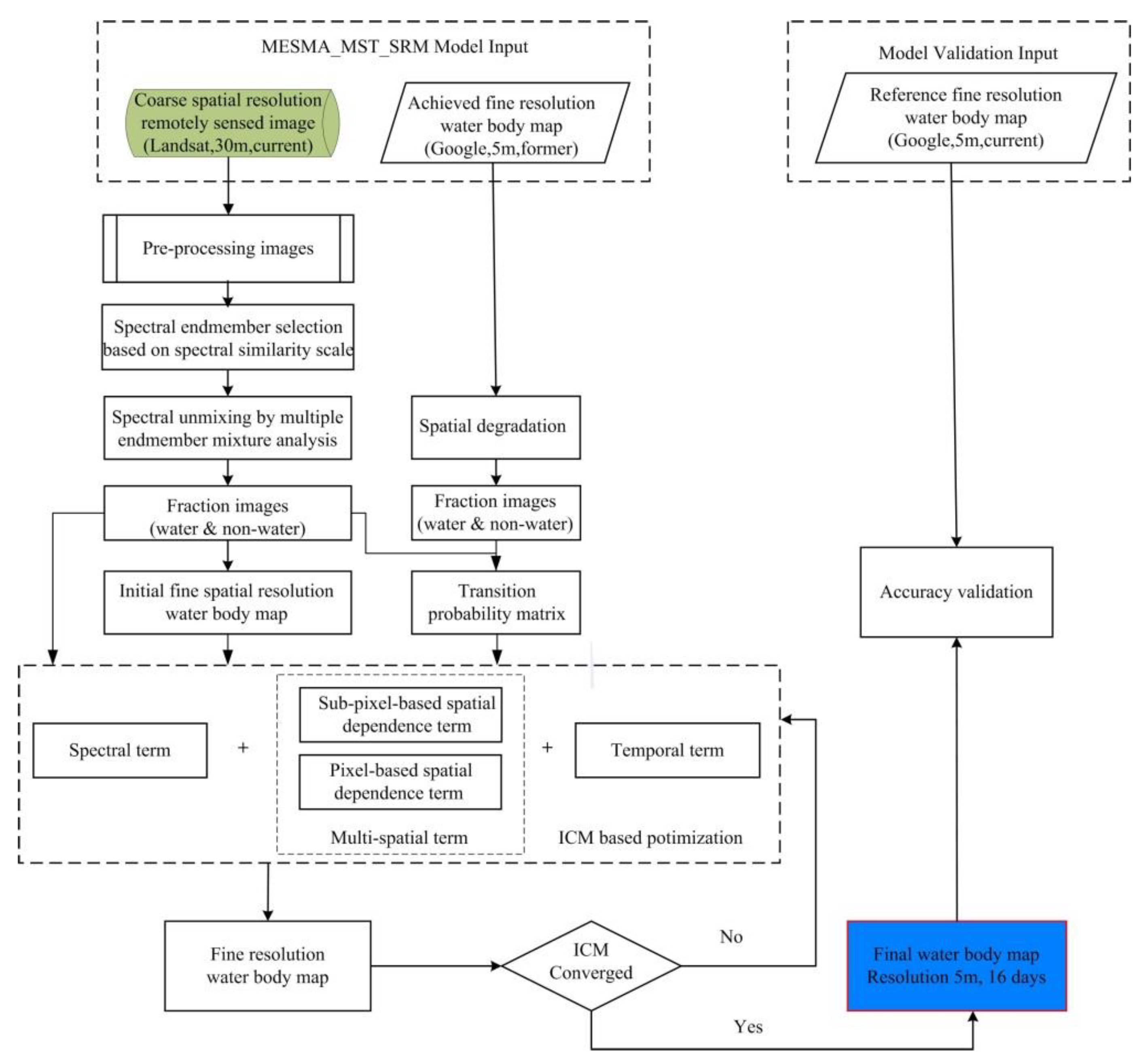
2.2.1. The Framework of MESMA_MST_SRM

The target of MESMA_MST_SRM is to generate a fine-resolution water body map from an input coarse-spatial-resolution remotely sensed image and the auxiliary information. In this study, achieved fine-resolution water body map was employed as the auxiliary information, and it is obtained from the fine-resolution remotely sensed image. Let Y be a coarse-spatial-resolution remotely sensed image at time T 2 containing M × N pixels with a spatial resolution of R. Let X p r e be the achieved fine-resolution water body map at time T 1 containing M × s × N × s pixels with a spatial resolution of r. In addition, X p r e and Y cover the same geographic area. The zoom factor s between X p r e and Y is R / r . Therefore, the resultant land cover water body map X at time T 2 contains M × s × N × s  pixels with a spatial resolution of r. Generally, the objective function of MESMA_MST_SRM includes three parts and is often formulated as
U ( X Y , X pre ) = U spectral ( X Y ) + α U spatial ( X ) + β U temporal ( X X pre )
where U ( X | Y , X p r e ) is the objective function for X, which is determined by Y and Xpre, U s p a t i a l ( X | Y ) , U s p a t i a l ( X ) and Utemporal are the spectral term, spatial term, and temporal term, respectively. α and β are the weighting coefficients that control the weights of the three energy terms. Based on the theory of Bayesian maximum a posteriori probability, the optimal resultant water body map X ^ is generated when U ( X | Y , X p r e ) reaches its minimum value. Therefore, the key issue of MESMA_MST_SRM is to define the three energy terms. The flowchart of the MESMA_MST_SRM method is shown in Figure 2, and the three energy terms are described in detail in the following text.

2.2.2. Spectral Term on SSS-Based MESMA

The spectral term in MESMA_MST_SRM aims to make the results conform to the input image Y. The fraction image, which is calculated through spectral unmixing of image Y and then applied to initialize the resultant fine-spatial-resolution water body map, is used to link the input image and the resultant map in this term. Therefore, the accuracy of the fraction images is vital for achieving the best results. Endmembers, which are regarded as the purest and smallest units in an image, play an important role in spectral unmixing and fraction image calculation. At present, popular endmember selection methods usually choose a fixed number of endmembers for each class and use their average spectral value to represent the spectral value of the land cover class. This kind of method is simple and easy to implement, but it ignores the spectral differences between the endmembers of different pixels.
To clearly describe the spectral differences within pixels and the similarities among pixels, a spectral similarity scale-based multiple-endmember spectral mixture analysis (SSS-based MESMA) model is employed in this study. In the SSS-based MESMA model, each coarse pixel in image Y has specific numbers of endmembers and endmember combinations. Suppose that C is the number of land cover classes; the specific steps of SSS-MESMA are as follows:
(1) Select the best-fit endmember for each coarse pixel in the land cover class ci based on the spectral similarity scale (SSS).
SSS is an index that integrates spectral brightness and spectral shape to evaluate the similarity of two spectral vectors, which can be calculated as [53]:
S S S i j c k = d 2 ( y i j , e c k ) + r ^ 2
where S S S i j c k represents the spectral similarity scale of the spectral vector of pixel p i j in Y and the spectral vector of the k-th candidate endmember in land cover class c; yij is the spectral vector of pixel p i j in Y; e c k is the spectral vector of the k-th candidate endmember in land cover class c; d represents the Euclidean distance between two spectral vectors; and r ^ is the correlation between y i j and e c k , which can be calculated as follows:
r ^ = 1 r 2 r 2 = ( 1 B 1 Σ B b = 1 ( y i j b μ y i j ) ( e c k b μ e c k ) σ y i j σ e c k ) 2 .
where μ y i j and σ y i j are the mean value and standard deviation of y i j , respectively, and μ e c k and σ e c k are the mean value and standard deviation of e c k ; B is the number of bands of Y.
In the SSS algorithm, a smaller SSS value means greater spectral similarity between pixel p i j and the candidate endmember. Therefore, according to the minimum SSS principle, the best-fit endmember for each coarse pixel at different land cover classes can be decided.
(2) Determine the number of endmembers and endmember combinations for each coarse pixel in Y. There are two classes (water and nonwater) in this study. Therefore, each coarse pixel in Y has two possible numbers of endmembers: one endmember and two endmembers. When the coarse pixel has one endmember, it could be water or nonwater. Generally, the endmember with the smallest SSS value is the optimal endmember. For cases with two endmembers, the endmember combination for a coarse pixel can only follow one case: partial water and partial nonwater. Finally, two endmember combinations for the coarse pixel are obtained.
(3) The endmember combinations are sequentially input into the linear mixed model to calculate the fraction value and the root mean square error (RMSE) value. The fraction value with the smallest RMSE is selected as the final fraction result. The linear mixture model (LMM) can be defined as follows:
f ˜ i j = a r g min | | y ij Ef ij | | 2
0 f i j , c 1 , c = 1 , , C
c = 1 C f i j , c = 1
where f ˜ i j represents the result of the linear mixture model for pixel p i j ; y i j is the spectral vector of coarse pixel p i j ; E is the optimal endmember spectral vector of all classes in pixel p i j ; f i j is the fraction vector of all classes in pixel p i j ; C is the number of land cover classes; and f i j , c is the proportion of class c in pixel p i j , which is in the range from 0 to 1.
(4) Repeat the above steps on the whole image and generate the final fraction image. The objective function of the spectral term can be defined as follows:
U s p e c t r a l ( X Y ) = i = 1 M j = 1 N c = 1 C y i j c E f i j c 2

2.2.3. Spatial Terms Based on Multiscale Spatiotemporal Dependence

The purpose of the spatial term is to provide class label information for the central subpixel through its neighbors. In general, a subpixel has two neighboring systems: pixel-scale and subpixel-scale neighboring systems. Suppose that the sizes of the neighborhood window at the pixel scale and subpixel scale are 3 and 5, respectively. The central subpixel has 8 neighboring pixels and 24 neighboring subpixels, which are used to help identify the class label for the central subpixel according to the maximum spatial dependence. Therefore, the spatial term includes two parts: a subpixel-based spatial dependence term and a pixel-based spatial dependence term.
U s p a t i a l ( X Y ) = δ U s p s p a t i a l ( X | Y ) + ( 1 δ ) U c p s p a t i a l ( X | Y )
(1) Spatial Term at the Subpixel Scale: The spatial term at the subpixel scale is used to keep the resultant map locally smoother. The maximum spatial dependence principle, which believes that a closer distance between the pixels may result in similar class labels, is employed in the spatial term. Under this principle, each central subpixel is affected by the surrounding w × w 1 neighboring subpixels, where w is the window size. The objective function of this term can be modeled as
U sp s p a t i a l ( X | Y ) = i = 1 M j = 1 N m = 1 s 2 l ϵ N s p ( a i j , m ) ϕ ( c 2 ( a i j , m ) , c 2 ( a l ) ) η ( a i j , m , a l )
where s is the zoom factor. a i j , m is the m-th subpixel in the coarse pixel p i j in Y, and N s p ( a i j , m ) is the subpixel-scale neighborhood system for a i j , m . a l is the l-th neighboring subpixel of a i j , m . c 2 ( a i j , m ) and c 2 ( a l ) are the class labels of subpixels a i j , m and a l in Y, respectively.
ϕ ( c 2 ( a i j , m ) , c 2 ( a l ) ) describes the spatial dependence between a i j , m and a l .
ϕ ( c 2 ( a i j , m ) , c 2 ( a l ) ) = { 1 c 2 ( a i j , m ) = c 2 ( a l ) 0 c 2 ( a i j , m ) c 2 ( a l )
The influence weight of neighboring subpixel a l on the central subpixel a i j , m varies with their distance. The Euclidean distance between a l and a i j , m is used to calculate the weight [54]:
η ( a i j , m , a l ) = 1 Ω exp ( 3 d ( a i j , m , a l ) / σ s p )
where d ( a i j , m , a l ) is the Euclidean distance between a i j , m and a l ; σ s p is a nonlinear distance attenuation parameter, and Ω is a normalization constant used to ensure that Σ l N s p L ( a i j , m ) ω ( a i j , m , a l ) = 1 .
(2) Spatial Term at the Pixel Scale: The spatial term at the pixel scale is helpful for the land cover class in terms of keeping the holistic distribution information at the pixel scale. The objective of this term is to maximize the spatial correlations between the central subpixel a i j and its neighboring w × w 1 coarse pixels p k , where w is the window size of the pixel neighborhood. The objective function of this term can be expressed as:
U c p s p a t i a l ( X | Y ) = i = 1 M j = 1 N m = 1 s 2 k ϵ N c p ( a i j , m ) ψ c 2 ( a i j , m ) ( p k ) ϖ ( a i j , m , p k )
where N c p ( a i j , m ) is the pixel-scale neighborhood system for a i j , m . ψ c 2 ( a i j , m ) ( p k ) represents the contribution coefficient of p k to the central subpixel in the class of c 2 ( a i j , m ) . The value of ψ c 2 ( a i j , m ) ( p k ) equals the fraction value of p k in Y. ϖ ( a i j , m , p k ) is the distance weight function, which represents the influence weight of the neighboring pixel p k on the central subpixel a i j , m , and the formula is based on a Gaussian function as follows:
ϖ ( a i j , m , p k ) = exp ( d 2 ( a i j , m , p k ) σ c p 2 )
where σ c p is a nonlinear distance attenuation parameter. d ( a i j , m , p k ) is the Euclidean distance between a i j , m and p k .

2.2.4. Temporal Term

The temporal term is used to obtain the prior temporal information from the archived high-spatial-resolution water body map. Suppose a i j , m is the m-th subpixel in the coarse pixel p i j in Y at time T 2 . a i j , m is affected by its temporal neighbor a k at time T 1 and the transition probability. Therefore, the objective function of the temporal term can be expressed as follows:
U temporal ( X X pre ) = i = 1 M j = 1 N m = 1 s 2 k N t ( a i j , m ) P ( c 2 ( a i j , m ) c 1 ( a k ) )
where N t ( a i j , m ) is the temporal neighborhood of the central subpixel a i j , m . P ( c 2 ( a i j , m ) | c 1 ( a k ) ) is the transition probability, which expresses the transition and change probabilities among different land cover classes from time T 1 to time T 2 . c 2 ( a i j , m ) is the class label of the central subpixel a i j , m at time T 2 . c 1 ( a k ) is the class label of pixel a k at time T 1 . The C × C transition probabilities make up the transition probability matrix T. In this study, two classes are contained in Y. The transition probability matrix T can be expressed as
T = [ P ( c 2 ( ) = ω l c 1 ( ) = ω l ) P ( c 2 ( ) = ω k c 1 ( ) = ω l ) P ( c 2 ( ) = ω l c 1 ( ) = ω k ) P ( c 2 ( ) = ω k c 1 ( ) = ω k ) ]
where c 1 ( ) and c 2 ( ) are the class labels of an arbitrary pixel in the previous fraction image and the current fraction image, respectively. P is calculated as [23]
P ( c 2 ( ) = ω ι c 1 ( ) = ω κ ) = i = 1 M × N × s 2 I ( c 1 ( a i ) = ω κ A N D c 2 ( a i ) = ω ι ) i = 1 M × N × s 2 I ( c 1 ( a i ) = ω k )
where c 1 ( a i ) is the class label of a i at time T 1 . Assume the value of c 1 ( a i ) is ω k ( k 1 , 2 , , C ) , if the transition probability from class ω k to class ω l ( l 1 , 2 , , C ) is high, the class label of the central subpixel a i j , m at time T 2 should be labeled as ω l . Otherwise, it should be labeled as ω k . I ( c 1 ( a i ) = ω k ) is an indicator function that is equal to 1 when c 1 ( a i ) = ω k and 0 otherwise.

2.3. Implementation of MESMA_MST_SRM and an Accuracy Evaluation

The objective function can be constructed after constructing the above three energy terms. Then, the final resultant high-resolution water body map is generated by optimizing the objective function in Formula (1). The iterative conditional model (ICM), a fast-converging algorithm, is adopted in the iterative process to realize the global energy minima. The implementation steps of the proposed MESMA_MST_SRM are as follows.
(1)
Preprocess the input images and initialize the parameters of the zoom factor, weight coefficients, and window size.
(2)
Choose the optimal endmembers for each pixel of the input image Y based on the SSS algorithm and decompose the input image Y. Then, obtain the fraction image for Y according to the MESMA model. Initialize the super-resolution (SR) map according to the fraction image.
(3)
Calculate the transition probability matrix based on Section 2.2.4 for subsequent use.
(4)
Update the class label of each subpixel in the SR map iteratively during the process of objective function optimization. The iteration procedure stops when the algorithm converges or reaches the set maximum number of iterations. The final class label is determined in the last iteration.
The overall accuracy (OA) and the correct labeling percentage for the unchanged pixels (PULC) are utilized for the accuracy evaluation in this study.

3. Results

3.1. Model Implementation and Comparative Experiments

Before the experiment, the model parameters needed to be initialized. The neighborhood window sizes at the pixel scale and subpixel scale were both set to seven, which meant that the center subpixel had 48 neighboring pixels and subpixels. Since the spatial resolution of the Landsat-8 imagery was 30 m and the spatial resolution of the Google Earth imagery was 5 m, the value of the scale factor was set to six. All of the algorithms were tested on an AMD Ryzen 7 4800H CPU with Radeon Graphics at 2.90 GHz, 16 GB of RAM, and MATLAB version R2018a.
Four additional methods were used for comparison; namely, hard classification (HC), mean endmembers and multiscale spatiotemporal dependence based on super-resolution mapping (MEAN_MST_SRM), multiple-endmember spectral mixture analysis and single-scale spatiotemporal dependence based on super-resolution mapping (MESMA_ST_SRM), and multiple-endmember spectral mixture analysis and multiscale spatial dependence based on super-resolution mapping without temporal terms (MESMA_MS_SRM). In HC, the class label value for each pixel is obtained from the fraction image, which is calculated by spectral unmixing at the pixel scale. MEAN_MST_SRM uses the average endmember for mixed-pixel spectral unmixing. MESMA_ST_SRM adopts a subpixel-based spatial dependence without considering its spatial pixel neighbors. MESMA_MS_SRM is a method based on MESMA and multiscale spatial terms, but it uses only one single remotely sensed image regardless of the temporal term.

3.2. The Results and Analysis

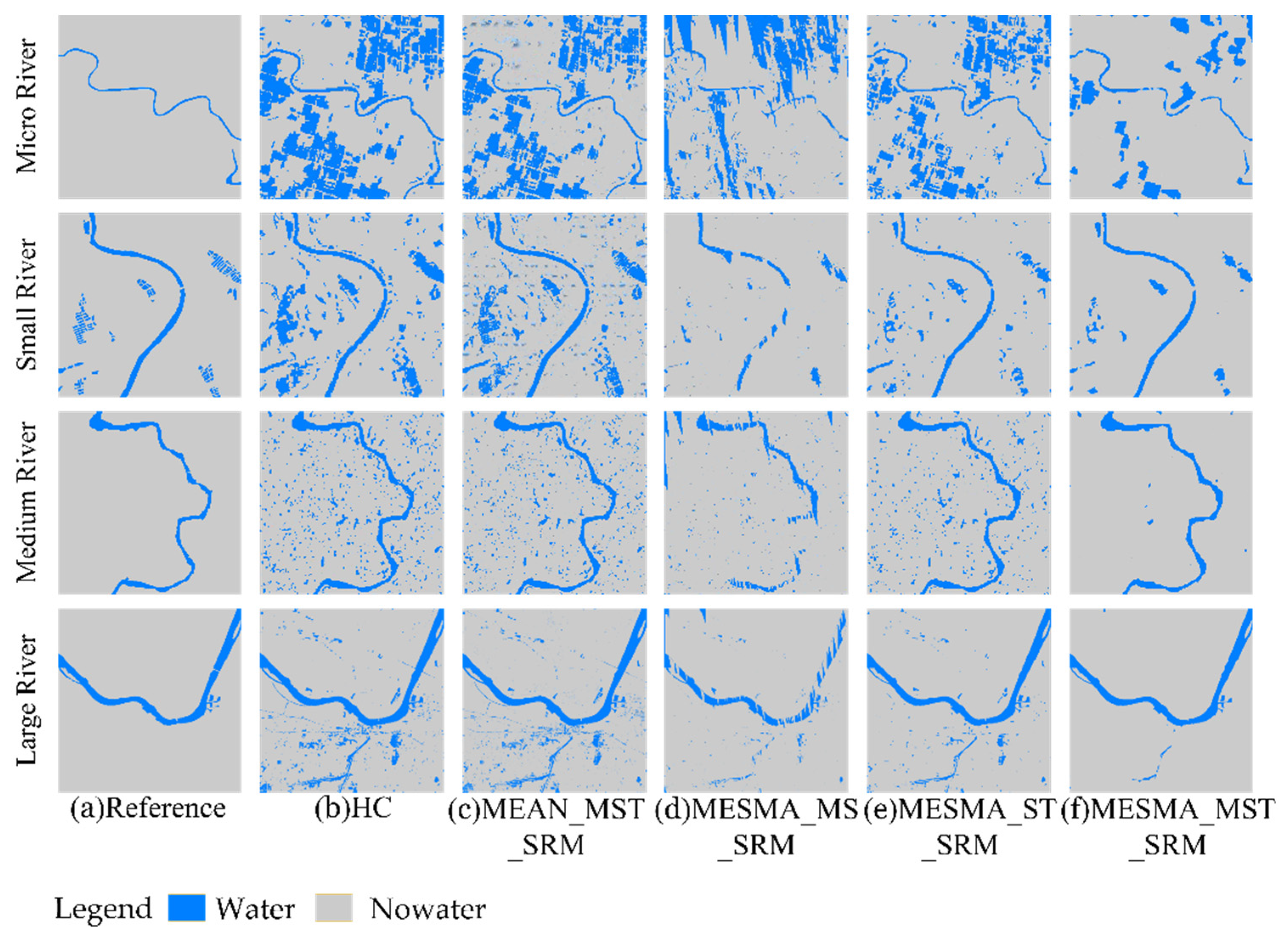
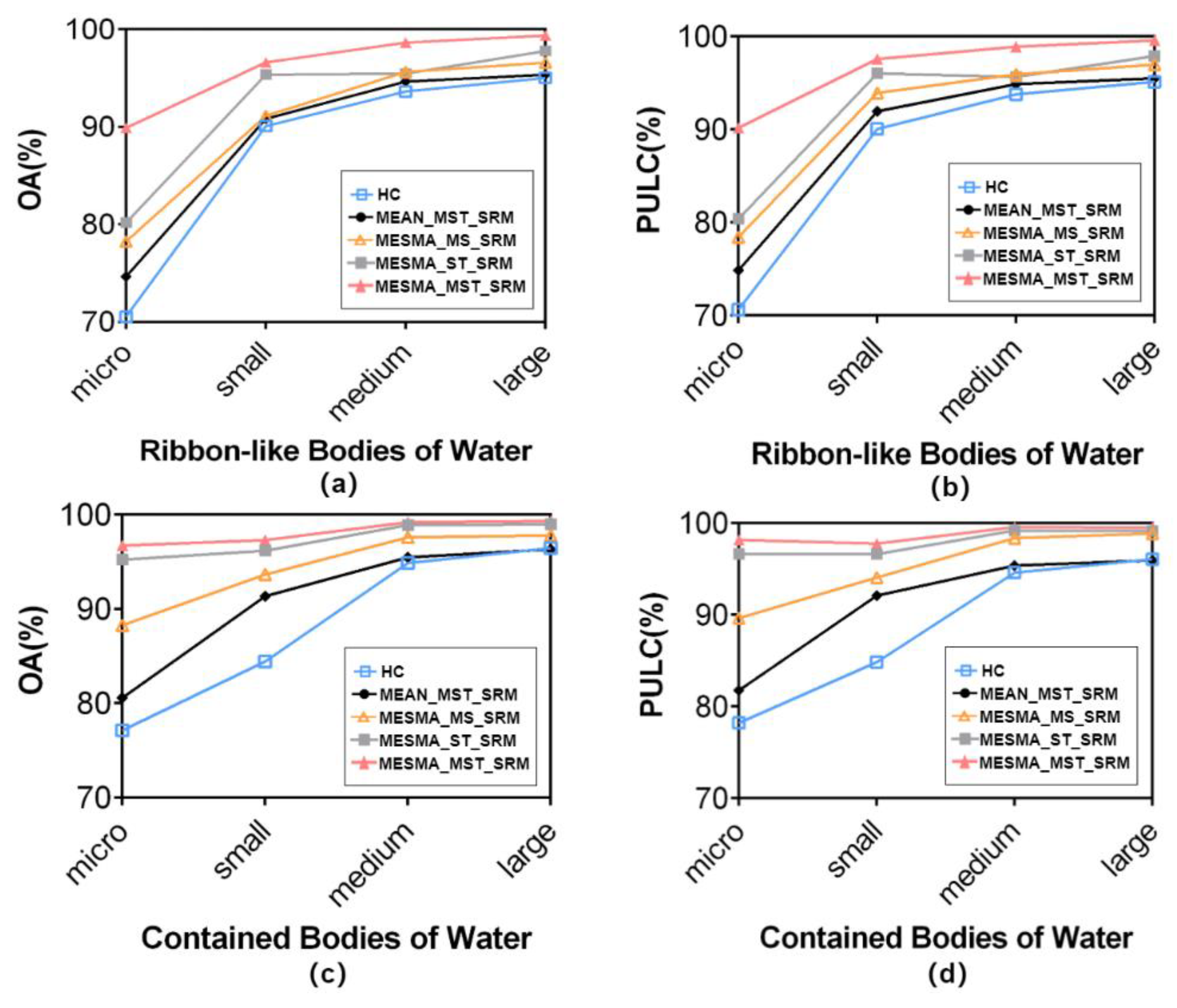
3.2.1. Ribbon-like Bodies of Water

In this section, four different ribbon-like bodies of water (such as rivers) were used for comparison purposes to verify the performance of the MESMA_MST_SRM method. In addition to MESMA_MST_SRM, the four other methods mentioned in Section B were also calculated for comparison. In the contrast experiments, the weighting coefficients of the three energy terms α and β were the optimal parameters. The other model parameters were initialized according to Section B. The resultant water body maps of the different methods for ribbon-like water bodies with different sizes are shown in Figure 3. The reference water body maps for the four different sizes of water (Figure 3a) were obtained from Google Earth images.
From the visual and qualitative perspectives of the results displayed in Figure 3, a smaller water body was more prone to being misclassified, and the noise was more serious. However, regardless of the size of the water body, the noise of the resultant water body map generated by the MESMA_MST_SRM method was the smallest, reflecting the superiority of this method.
In Figure 3b, the resultant water body map produced by the HC-based method has jagged water body boundaries and many fragmentary noise patterns. The main reason for this is that HC is a pixel-scale classification method that cannot solve the spatial uncertainty caused by mixed pixels and cannot correctly determine the spatial distribution of water and nonwater. Finally, some nonwater pixels were incorrectly labeled as belonging to the water class. Although the unmixing and allocation processes were based on the subpixel scale in the MEAN_MST_SRM method, the results shown in Figure 3c still have excessive amounts of noise because of the use of the average endmember for mixed-pixel spectral unmixing. Actually, the average spectral values of the candidate endmembers could not correctly indicate the spectral value of each mixed pixel, which led to low spectral unmixing and fraction image accuracies. Therefore, the accuracy of the results was low. The resulting water body maps in Figure 3d have poor spatial continuity and smoothness due to the lack of a temporal term. Generally, a temporal term can provide prior spatial pattern information from a previous high-spatial-resolution water body map. With the help of the prior spatial pattern information and the MESMA-based unmixing method, the MESMA_ST_SRM method (Figure 3e) could provide better results than those of the former methods. However, there are still some fragmented noise patterns in the MESMA_ST_SRM results due to the lack of holistic spatial pattern constraints at the pixel scale. Compared with the above results, the resultant water body map generated by MESMA_MST_SRM (Figure 3f) is closer to the reference water body map overall and in terms of detail, which is mainly due to the MESMA-based endmember selection model and the multiscale spatial dependence model. With the help of the MESMA-based endmember selection model, each coarse pixel has specific endmember combinations, which can improve the unmixing accuracy of coarse pixels and improve the mapping accuracy. Moreover, by using the center subpixel of the multiscale spatial dependence model, more prior spatial pattern information could be obtained in the location process from the neighboring pixels and subpixels.
The accuracy statistics comparison for different ribbon-like water bodies is shown in Table 2. For these four different sizes of water bodies, the OA and PULC values obtained by the MESMA_MST_SRM method are the highest. Overall, the PULC value is higher than the OA value. This is because unchanged pixels can directly inherit the spatial pattern from the former Google Earth water body map. Hence, the correct labeling percentage for the unchanged pixels (PULC) is higher. The “improvement rate of OA” was used here to compare the improvement rates of the proposed MESMA_MST_SRM approach and other methods. For example, the “improvement rate of OA” between MESMA_MST_SRM and HC on the Tongshun River (micro water body) was calculated as (89.9099–70.5453)/70.5453. The results showed that more obvious improvements occurred when those methods were executed on smaller water bodies. In practice, small water bodies are more difficult to extract than larger bodies. This is because in medium-spatial-resolution satellite images, small water bodies often cover only a few pixels or even less than one pixel. It is difficult to extract water bodies from only a few pixels or a single pixel because of the serious phenomenon of mixed pixels. Fortunately, the MESMA_MST_SRM method obtained a relatively high accuracy.

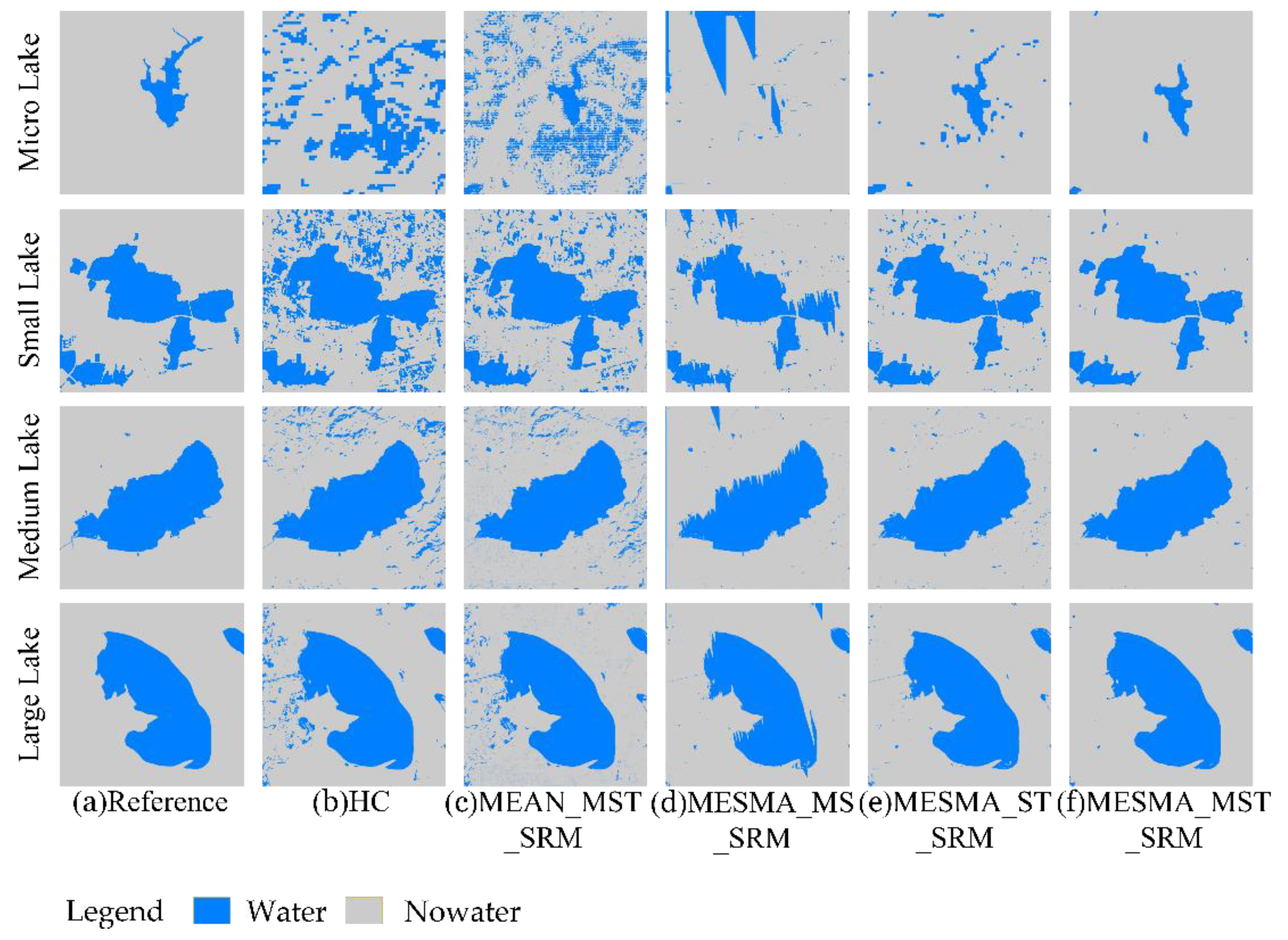
3.2.2. Contained Bodies of Water

Four contained bodies of water with different sizes were used for comparative experiments to verify the validity of the proposed MESMA_MST_SRM method. The resultant water body maps produced by different methods are displayed in Figure 4.
As shown in Figure 4b, the resultant water maps of HC have considerable noise, and many nonwater patches are wrongly divided into water bodies. It is difficult to identify the shapes of micro water bodies due to the lack of spatial patterns and the pixel-based classification approach of HC. For MEAN_MST_SRM (Figure 4c), the noise is still serious, especially for micro and small water bodies. This is because the average endmember could not correctly express the spectral differences and similarities within pixels, resulting in a low unmixing accuracy and inaccurate fraction images.
In Figure 4d, by using the MESMA model, noise was obviously suppressed. However, due to the lack of prior spatial pattern information, there are obvious zigzag marks at the water boundary. By incorporating the previous Google Earth water body map, the boundary of the water body map generated by MESMA_ST_SRM (Figure 4e) is relatively smooth. However, for small or micro water bodies, there is still much noise. In contrast, the results obtained by the MESMA_MST_SRM method are closest to the reference map, the noise is very low, and the water boundary is smooth (Figure 4f). It is worth mentioning that the MESMA_MST_SRM method also performed well on the four sizes of contained bodies of water, such as lakes, even for small or micro bodies.
The quantitative results of the comparison experiments are shown in Table 3. The MESMA_MST_SRM method had the highest OA and PULC values for each water body size. When the model was applied to micro or small water bodies, the improvement rate of OA was significantly high. The results on the contained bodies of water were consistent with those obtained for the ribbon-like bodies of water, reflecting the superiority and universality of the proposed MESMA_MST_SRM method.

4. Discussion

4.1. Effects of the Weighting Coefficients

The weighting coefficients α and β, which were used to control the weights of the three energy terms, had an important influence on the mapping results. Proper weight coefficients can better integrate the three energy terms and generate highly accurate results. Otherwise, these coefficients may lead to poor objective function performance and inaccurate results. South Lake was selected as an example to illustrate the influence of the weight coefficients on the results, and four representative resultant water body maps in Figure 5 were chosen to demonstrate their influence. Figure 5a shows considerable noise, and the boundary is unsmooth. The main reason for this is that when the value of α equals 0, the spatial energy term does not work. In contrast, when the value of α is large (for example, 10,000 in Figure 5b but the value of β is set to 0), the boundary is obviously serrated. In this case, the temporal energy term is missing, and the former fine-resolution water body map is invalid, leading to a lack of spatial patterns and jiggle boundaries. In Figure 5c, the value of α is 8000, and the value of β is only 10. In this case, although the three energy terms can all work, the result is still not very good. When α is large and β is small, the spatial term plays a dominant role, and the prior information of the former fine-resolution water body map is not fully utilized. Parameter settings, such as those utilized in this case, are also regarded as inappropriate combinations. In this study, the appropriate and optimal values of α and β were set by trial and error; for example, 8000 and 2500 were the best combinations here. Compared with the previous three results, the result in Figure 5d is best, with smooth boundaries and low noise.
Table 4 shows the accuracy statistics of South Lake achieved by MESMA_MST_SRM with different weighting coefficients. When the value of α was small, the values of overall accuracy (OA) changed very little regardless of the value of β because the model did not make full use of the spatial correlations between pixels and subpixels. In contrast, when the value of β was small, a large value of α led to a low OA because of the dominance of the spatial term and the lack of prior spatial information. When β was 0, the smallest value of OA was only 89%. As β increases, the previous image can provide more spatial prior information for the locating process, and the OA reaches its best value at the optimal combination of α and β. In general, the value of PULC is higher than that of OA. This is because OA represents the overall accuracy, including the accuracies of both changed and unchanged pixels, while PULC only represents the accuracy of unchanged pixels. Unchanged pixels can directly inherit the spatial pattern from a previous high-resolution water body map; therefore, they are easier to correctly classify.

4.2. Effect of the Water Body Type

The results of water body mappings are also affected by the type of water body. The different shapes or sizes of water bodies may lead to different water extraction accuracies. To explore the influence of water types on the results, the extraction results of eight different types of water bodies under different methods were compared, and the resulting curves are shown in Figure 6.
In Figure 6, the accuracy curves show upward trends for both ribbon-like bodies of water and contained bodies of water under all five comparative methods. When the water body size reaches a medium value, the curve begins to rise steadily and slowly. Moreover, large water has an obviously higher accuracy value than micro water. For the HC method, the OA value for large bodies of water can exceed 96%, but for micro water bodies, it is only approximately 70%. The same phenomenon also exists in the other four methods. The main reason for this is that for a micro river, the average river width is 50 m, which means that it only covers less than two pixels in a Landsat image. When pixel-based methods such as HC are applied, a pixel is classified as a water body once more than 50% of the pixel area is covered by water. As a consequence, the OA value is very low. Generally, in medium-resolution satellite images, micro or small water bodies account for only a few pixels or even less than one pixel, which makes it very difficult to accurately extract these water bodies and monitor water changes. In contrast, medium or large water bodies usually have few changes and easily yield high extraction accuracy.
In terms of shape, the accuracy of ribbon-like bodies of water (such as rivers) is generally less than that of contained bodies of water (such as lakes) with the same size, especially when the water size is micro. For example, under the MESMA_MST_SRM method, the OA value of micro ribbon-like bodies of water was only 89.9%, while that of micro contained bodies of water was 96.7%. This phenomenon also exists in the other four methods, which indicates that micro ribbon-like bodies of water are harder to extract than micro contained bodies of water.
Overall, different mean widths of ribbon-like bodies of water and different areas of contained bodies of water had important effects on the results. However, compared to the other four methods, the MESMA_MST_SRM method performed best in extracting different shapes and sizes of water. For micro ribbon-like bodies of water, the OA of MESMA_MST_SRM improved by 27.45% over that of HC, and for micro contained bodies of water, the OA of MESMA_MST_SRM improved by 25.41% over that of HC. For large water bodies, the OA value generated by the MESMA_MST_SRM method was still higher than that of the HC method, which indicates the superiority and robustness of the proposed method.

4.3. Effect of the Zoom Factor

The zoom factor s reflects the spatial resolution ratio between the coarse image Y and the resultant water body map X. For a certain coarse image Y, the larger the value of zoom factor s is, the higher the spatial resolution of the obtained water body map X. However, if the value of s is too large, the accuracy result may decrease. To verify the influence of the zoom factor s on the results, water extraction experiments under different zoom factors of s = 3, s = 6, s = 15, s = 30 and are used for comparison (see Figure 7).
As shown in Figure 7, in the five comparative experiments, the image noise increased with an increasing zoom factor. The noise of HC and MEAN-MST-SRM is significantly higher than that of the other three methods, which is mainly due to the use of the mean endmember in these two methods. In contrast, the other three MESMA-based methods have relatively less noise. At the same zoom scale, the MESMA-MS-SRM method has the least noise and the best boundary smoothness, which reflects the advantages of multiscale spatiotemporal.
However, even for the best performing MESMA-MS-SRM, the noise increases with the increasing zoom factor, especially when the scales are 15 and 30. The quantitative results (Table 5) also manifest this phenomenon. The zoom factor increases, and the overall accuracy decreases because the uncertainty increases when the value of s increases. The overall accuracy of the HC method changes little at the four different zoom scales, mainly because the HC method is a pixel algorithm. The zoom factor increases, and the overall accuracy of the MEAN_MST_SRM method decreases rapidly. The value of OA is lower than 90% when the scale factor is 15, which indicates that the mean endmember has great uncertainty on a large zoom factor. The OA and PULC values of MESMA_MST_SRM are all higher than those of the other four methods at different zoom scales. However, the overall accuracy also decreased as the zoom factor increased for MESMA_MST_SRM. When the zoom factor is 30, the overall accuracy is approximately 96%. Considering the visual and quantitative results, when s equals six, better results can be obtained, and the computational complexity is relatively small.

5. Conclusions

In this study, a super-resolution water body mapping method based on MESMA and multiscale spatiotemporal dependence was proposed. The MESMA_MST_SRM method can be applied to water body mapping with high spatio-temporal resolution. It makes use of the time advantage of medium spatial resolution to make up for the time shortage of high spatial resolution, so as to generate a high spatio-temporal resolution water body map. Specifically, in the proposed MESMA_MST_SRM method, each coarse pixel has a specific endmember set according to the lowest sum of the spectral similarity scale (SSS) values, which allows different pixels to have different types and numbers of endmember combinations. We verified the potential of SSS-based MESMA in water mapping. The results showed that, based on the MESMA model, spectral variability among the given pixels was fully considered, and high-accuracy fraction images could be generated. Moreover, the MESMA _MST_SRM method was carried out under both pixel-based and subpixel-based spatiotemporal dependence; it not only maintained the overall structure information but also presented the detailed information of each water body. As a result, the proposed MESMA_MST_SRM method not only reduces the spectral unmixing error and improves the accuracy of the fraction image but also provides a better spatial pattern than that obtained with single-level spatial dependence.
The proposed MESMA_MST_SRM approaches were tested by using eight types of water with different types and sizes via a comparison with four other methods, either under the mean endmember selection rule or under single-level spatial dependence. The eight experimental results showed that the proposed MESMA_MST_SRM method had the highest OA values for the eight types of water, and the water body maps generated by MESMA_MST_SRM had relatively smooth boundaries and more detailed water information. By using MESMA_MST_SRM, the OA values on large river-like or lake-like water bodies reached 99%, and for micro river-like water bodies, the OA improvement rate reached 27% over the accuracy of the HC method. The high accuracy and comparability for different types of water bodies indicated that MESMA_MST_SRM is a promising method for super-resolution water body mapping.
However, as it is discussed in Section 4, the zoom factor will affect the results of water body mapping. On the one hand, it cannot obtain a high spatial resolution water body map at a small zoom factor. On the other hand, when the value of zoom factor is large, the accuracy is limited and the computational complexity increases. Considering the accuracy and complexity, when the zoom factor is equal to six, the comprehensive performance of the method is better. Thus, a water body map at 16-daily intervals and a 5 m resolution from Landsat and Google Earth imagery can be generated by using MESMA_MST_SRM.

Author Contributions

X.Y. and L.W. conceived and designed the experiments; Q.C. and M.Y. performed the experiments; X.Y. and Q.C. analyzed the results. The manuscript was written by X.Y. and Q.C. and was improved by the contributions of all of the coauthors. All authors have read and agreed to the published version of the manuscript.

Funding

The research was funded by the National Natural Science Foundation of China (Grant No. 42001308, No. U21A2013 and No. 41925007), in part by Science and Technology Support Project of Department of Natural Resources of Hubei Province (ZRZY2022KJ03) and in part by the State Key Laboratory of Biogeology and Environmental Geology, China University of Geosciences (Grant No. GBL12107).

Institutional Review Board Statement

Not applicable.

Informed Consent Statement

Not applicable.

Conflicts of Interest

The authors declare no conflict of interest.

References

  1. Wang, J.; Song, C.; Reager, J.T.; Yao, F.; Famiglietti, J.S.; Sheng, Y.; MacDonald, G.M.; Brun, F.; Schmied, H.M.; Marston, R.A.; et al. Recent global decline in endorheic basin water storages. Nat. Geosci. 2018, 11, 926–932. [Google Scholar] [CrossRef] [PubMed] [Green Version]
  2. Wang, X.; Xiao, X.; Zou, Z.; Dong, J.; Qin, Y.; Doughty, R.B.; Menarguez, M.A.; Chen, B.; Wang, J.; Ye, H.; et al. Gainers and losers of surface and terrestrial water resources in China during 1989–2016. Nat. Commun. 2020, 11, 1–12. [Google Scholar] [CrossRef]
  3. Tzanakakis, V.A.; Paranychianakis, N.V.; Angelakis, A.N.J.W. Water supply and water scarcity. Water 2020, 12, 2347. [Google Scholar] [CrossRef]
  4. Xu, L.; Abbaszadeh, P.; Moradkhani, H.; Chen, N.; Zhang, X. Continental drought monitoring using satellite soil moisture, data assimilation and an integrated drought index. Remote Sens. Environ. 2020, 250, 112028. [Google Scholar] [CrossRef]
  5. Wu, J.; Sun, Z. Evaluation of shallow groundwater contamination and associated human health risk in an alluvial plain impacted by agricultural and industrial activities, mid-west China. Expo. Health 2015, 8, 311–329. [Google Scholar] [CrossRef]
  6. Loucks, D.P.; van Beek, E. Water Resources Planning and Management: An Overview. In Water Resource Systems Planning and Management; Springer: Cham, Switzerland, 2017; pp. 1–49. [Google Scholar]
  7. Feyisa, G.L.; Meilby, H.; Fensholt, R.; Proud, S.R. Automated Water Extraction Index: A new technique for surface water mapping using Landsat imagery. Remote Sens. Environ. 2014, 140, 23–35. [Google Scholar] [CrossRef]
  8. Ryu, J.H.; Won, J.S.; Min, K.D. Waterline extraction from Landsat TM data in a tidal flat: A case study in Gomso Bay, Korea. Remote Sens. Environ. 2002, 83, 442–456. [Google Scholar] [CrossRef]
  9. Chen, Q.; Zhang, Y.; Ekroos, A.; Hallikainen, M. The role of remote sensing technology in the EU water framework directive (WFD). Environ. Sci. Policy. 2004, 7, 267–276. [Google Scholar] [CrossRef]
  10. Williamson, C.E.; Saros, J.E.; Vincent, W.F.; Smol, J.P. Lakes and reservoirs as sentinels, integrators, and regulators of climate change. Limnol. Oceanogr. 2009, 54, 2273–2282. [Google Scholar] [CrossRef]
  11. Birk, S.; Ecke, F. The potential of remote sensing in ecological status assessment of coloured lakes using aquatic plants. Ecol. Indic. 2014, 46, 398–406. [Google Scholar] [CrossRef]
  12. Reyjol, Y.; Argillier, C.; Bonne, W.; Borja, A.; Buijse, A.D.; Cardoso, A.C.; Daufresne, M.; Kernan, M.; Ferreira, M.T.; Poikane, S.; et al. Assessing the ecological status in the context of the European Water Framework Directive: Where do we go now? Sci. Total Environ. 2014, 497–498, 332–344. [Google Scholar] [CrossRef] [PubMed]
  13. Acharya, T.D.; Subedi, A.; Lee, D.H. Evaluation of water indices for surface water extraction in a Landsat 8 scene of Nepal. Sensors 2018, 18, 2580. [Google Scholar] [CrossRef] [PubMed] [Green Version]
  14. McFeeters, S.K. The use of the Normalized Difference Water Index (NDWI) in the delineation of open water features. Int. J. Remote Sens. 1996, 17, 1425–1432. [Google Scholar] [CrossRef]
  15. Yao, F.; Wang, C.; Dong, D.; Luo, J.; Shen, Z.; Yang, K. High-resolution mapping of urban surface water using ZY-3 multi-spectral imagery. Remote Sens. 2015, 7, 12336–12355. [Google Scholar] [CrossRef] [Green Version]
  16. Acharya, T.D.; Lee, D.H.; Yang, I.T.; Lee, J.K. Identification of water bodies in a Landsat 8 OLI image using a J48 decision tree. Sensors 2016, 16, 1075. [Google Scholar] [CrossRef] [Green Version]
  17. Rokni, K.; Ahmad, A.; Solaimani, K.; Hazini, S. A new approach for surface water change detection: Integration of pixel level image fusion and image classification techniques. Int. J. Appl. Earth Obs. Geoinf. 2015, 34, 226–234. [Google Scholar] [CrossRef]
  18. Pekel, J.F.; Vancutsem, C.; Bastin, L.; Clerici, M.; Vanbogaert, E.; Bartholomé, E.; Defourny, P. A near real-time water surface detection method based on HSV transformation of MODIS multi-spectral time series data. Remote Sens. Environ. 2014, 140, 704–716. [Google Scholar] [CrossRef] [Green Version]
  19. Sun, Y.; Huang, S.; Li, J.; Li, X.; Ma, J.; Li, S.; Wang, H. Dynamic monitoring of Poyang Lake water body area using MODIS images between 2000 and 2014. In Proceedings of the International Conference on Intelligent Earth Observing and Applications, Guilin, China, 9 December 2015. [Google Scholar]
  20. Zhao, J.; Li, J.; Zhang, C.; Du, S.; Yao, Y.; Wang, Q.; Zhao, S. Estimating and Validating Wheat Leaf Water Content with Three MODIS Spectral Indexes: A Case Study in Ningx ia Plain, China. J. Agric. Sci. Technol. 2018, 18, 387–398. [Google Scholar]
  21. Rao, P.; Jiang, W.; Hou, Y.; Chen, Z.; Jia, K. Dynamic change analysis of surface water in the Yangtze River Basin based on MODIS products. Remote Sens. 2018, 10, 1025. [Google Scholar] [CrossRef] [Green Version]
  22. Pekel, J.-F.; Cottam, A.; Gorelick, N.; Belward, A.S. High-resolution mapping of global surface water and its long-term changes. Nature 2016, 540, 418–422. [Google Scholar] [CrossRef]
  23. Tulbure, M.G.; Broich, M.; Stehman, S.V.; Kommareddy, A. Surface water extent dynamics from three decades of seasonally continuous Landsat time series at subcontinental scale in a semi-arid region. Remote Sens. Environ. 2016, 178, 142–157. [Google Scholar] [CrossRef]
  24. Tao, S.; Fang, J.; Zhao, X.; Zhao, S.; Shen, H.; Hu, H.; Tang, Z.; Wang, Z.; Guo, Q. Rapid loss of lakes on the Mongolian Plateau. Proc. Natl. Acad. Sci. USA 2015, 112, 2281–2286. [Google Scholar] [CrossRef] [Green Version]
  25. Feng, M.; Sexton, J.O.; Channan, S.; Townshend, J.R. A global, high-resolution (30-m) inland water body dataset for 2000: First results of a topographic–spectral classification algorithm. Int. J. Digit. Earth. 2016, 9, 113–133. [Google Scholar] [CrossRef] [Green Version]
  26. Yamazaki, D.; Trigg, M.A.; Ikeshima, D. Development of a global~90 m water body map using multi-temporal Landsat images. Remote Sens. Environ. 2015, 171, 337–351. [Google Scholar] [CrossRef]
  27. Xia, H.; Zhao, J.; Qin, Y.; Yang, J.; Cui, Y.; Song, H.; Ma, L.; Jin, N.; Meng, Q. Changes in water surface area during 1989–2017 in the Huai River Basin using Landsat data and Google earth engine. Remote Sens. 2019, 11, 1824. [Google Scholar] [CrossRef] [Green Version]
  28. Gao, H.; Birkett, C.; Lettenmaier, D.P. Global monitoring of large reservoir storage from satellite remote sensing. Water Resour. Res. 2012, 48, W09504. [Google Scholar] [CrossRef] [Green Version]
  29. Foody, G.; Cox, D. Sub-pixel land cover composition estimation using a linear mixture model and fuzzy membership functions. Remote Sens. 1993, 15, 619–631. [Google Scholar] [CrossRef]
  30. Ling, F.; Boyd, D.; Ge, Y.; Foody, G.M.; Li, X.; Wang, L.; Zhang, Y.; Shi, L.; Shang, C.; Li, X.; et al. Measuring river wetted width from remotely sensed imagery at the subpixel scale with a deep convolutional neural network. Water Resour. Res. 2019, 55, 5631–5649. [Google Scholar] [CrossRef]
  31. Kasetkasem, T.; Arora, M.K.; Varshney, P.K. Super-resolution land cover mapping using a Markov random field based approach. Remote Sens. Environ. 2005, 96, 302–314. [Google Scholar] [CrossRef]
  32. Ling, F.; Du, Y.; Xiao, F.; Xue, H.; Wu, S. Super-resolution land-cover mapping using multiple sub-pixel shifted remotely sensed images. Int. J. Remote Sens. 2010, 31, 5023–5040. [Google Scholar] [CrossRef]
  33. Li, X.; Ling, F.; Foody, G.M.; Ge, Y.; Zhang, Y.; Wang, L.; Shi, L.; Li, X.; Du, Y. Spatial-temporal super-resolution land cover mapping with a local spatial-temporal dependence model. IEEE Trans. Geosci. Remote Sens. 2019, 57, 4951–4966. [Google Scholar] [CrossRef]
  34. Ling, F.; Li, X.; Du, Y.; Xiao, F. Super-resolution land cover mapping with spatial–temporal dependence by integrating a former fine resolution map. IEEE J. Sel. Top. Appl. Earth Obs. Remote Sens. 2014, 7, 1816–1825. [Google Scholar] [CrossRef]
  35. Li, X.; Du, Y.; Ling, F. Super-resolution mapping of forests with bitemporal different spatial resolution images based on the spatial-temporal Markov random field. IEEE J. Sel. Top. Appl. Earth Obs. Remote Sens. 2013, 7, 29–39. [Google Scholar] [CrossRef]
  36. Li, L.; Chen, Y.; Xu, T.; Liu, R.; Shi, K.; Huang, C. Super-resolution mapping of wetland inundation from remote sensing imagery based on integration of back-propagation neural network and genetic algorithm. Remote Sens. Environ. 2015, 164, 142–154. [Google Scholar] [CrossRef]
  37. Ling, F.; Xiao, F.; Du, Y.; Xue, H.; Ren, X. Waterline mapping at the subpixel scale from remote sensing imagery with high-resolution digital elevation models. Int. J. Remote Sens. 2008, 29, 1809–1815. [Google Scholar] [CrossRef]
  38. Zhang, Y.; Atkinson, P.M.; Li, X.; Ling, F.; Wang, Q.; Du, Y. Learning-based spatial–temporal super-resolution mapping of forest cover with modis images. IEEE Trans. Geosci. Remote Sens. 2016, 55, 600–614. [Google Scholar] [CrossRef]
  39. Ling, F.; Li, X.; Foody, G.M.; Boyd, D.; Ge, Y.; Li, X.; Du, Y. Monitoring surface water area variations of reservoirs using daily MODIS images by exploring sub-pixel information. ISPRS J. Photogramm. Remote Sens. 2020, 168, 141–152. [Google Scholar] [CrossRef]
  40. Yang, X.; Li, Y.; Wei, Y.; Chen, Z.; Xie, P. Water Body Extraction from Sentinel-3 Image with Multiscale Spatiotemporal Super-Resolution Mapping. Water 2020, 12, 2605. [Google Scholar] [CrossRef]
  41. Tran, H.; Nguyen, P.; Ombadi, M.; Hsu, K.; Sorooshian, S.; Andreadis, K. Improving hydrologic modeling using cloud-free MODIS flood maps. J. Hydrometeorol. 2019, 20, 2203–2214. [Google Scholar] [CrossRef] [Green Version]
  42. Osorio, J.D.G.; Galiano, S.G.G. Development of a sub-pixel analysis method applied to dynamic monitoring of floods. Int. J. Remote Sens. 2011, 33, 2277–2295. [Google Scholar] [CrossRef]
  43. Mertens, K.C.; de Baets, B.; Verbeke, L.P.; de Wulf, R.R. A sub-pixel mapping algorithm based on sub-pixel/pixel spatial attraction models. Int. J. Remote Sens. 2007, 27, 3293–3310. [Google Scholar] [CrossRef]
  44. Zhang, Y.; Du, Y.; Ling, F.; Wang, X.; Li, X. Spectral–spatial based sub-pixel mapping of remotely sensed imagery with multi-scale spatial dependence. Int. J. Remote Sens. 2015, 36, 2831–2850. [Google Scholar] [CrossRef]
  45. Roberts, D.A.; Gardner, M.; Church, R.; Ustin, S.; Scheer, G.; Green, R. Mapping chaparral in the Santa Monica Mountains using multiple endmember spectral mixture models. Remote Sens. Environ. 1998, 65, 267–279. [Google Scholar] [CrossRef]
  46. Franke, J.; Roberts, D.A.; Halligan, K.; Menz, G. Hierarchical multiple endmember spectral mixture analysis (MESMA) of hyperspectral imagery for urban environments. Remote Sens. Environ. 2009, 113, 1712–1723. [Google Scholar] [CrossRef]
  47. Fernandez-Manso, A.; Quintano, C.; Roberts, D.A. Burn severity influence on post-fire vegetation cover resilience from Landsat MESMA fraction images time series in Mediterranean forest ecosystems. Remote Sens. Environ. 2016, 184, 112–123. [Google Scholar] [CrossRef]
  48. Fan, F.; Deng, Y. Enhancing endmember selection in multiple endmember spectral mixture analysis (MESMA) for urban impervious surface area mapping using spectral angle and spectral distance parameters. Int. J. Appl. Earth Obs. Geoinf. 2014, 33, 290–301. [Google Scholar] [CrossRef]
  49. Bartout, P.; Touchart, L.; Terasmaa, J.; Choffel, Q.; Marzecova, A.; Koff, T.; Kapanen, G.; Qsair, Z.; Maleval, V.; Millot, C.; et al. A new approach to inventorying bodies of water, from local to global scale. Erde 2015, 146, 245–258. [Google Scholar]
  50. Downing, J.A. Emerging global role of small lakes and ponds: Little things mean a lot. Limnetica. 2009, 29, 9–24. [Google Scholar] [CrossRef]
  51. Minns, C.K.; Moore, J.E.; Shuter, B.J.; Mandrak, N.E. A preliminary national analysis of some key characteristics of Canadian lakes. Can. J. Fish. Aquat. Sci. 2008, 65, 1763–1778. [Google Scholar] [CrossRef] [Green Version]
  52. Downing, J.A.; Prairie, Y.T.; Cole, J.J.; Duarte, C.M.; Tranvik, L.J.; Striegl, R.G.; McDowell, W.H.; Kortelainen, P.; Caraco, N.F.; Melack, J.M.; et al. The global abundance and size distribution of lakes, ponds, and impoundments. Limnol. Oceanogr. 2006, 51, 2388–2397. [Google Scholar] [CrossRef] [Green Version]
  53. Granahan, J.; Sweet, J. An evaluation of atmospheric correction techniques using the spectral similarity scale. In Proceedings of the International Geoscience and Remote Sensing Symposium, Sydney, NSW, Australia, 9–13 July 2001; pp. 2022–2024. [Google Scholar]
  54. Park, S.C.; Park, M.K.; Kang, M.G. Super-resolution image reconstruction: A technical overview. IEEE Signal Process. Mag. 2003, 20, 21–36. [Google Scholar] [CrossRef] [Green Version]
Figure 1. Data used in the experiments: (1) (a1c1) are the data for the micro river; (2) (a2c2) are the data for the small river; (3) (a3c3) are the data for the medium river; (4) (a4c4) are the data for the large river; (5) (a5c5) are the data for the micro lake; (6) (a6c6) are the data for the small lake; (7) (a7c7) are the data for the medium lake; and (8) (a8c8) are the data for the large lake.
Remotesensing 14 02050 g001
Figure 2. Flowchart of the MESMA_MST_SRM method.
Remotesensing 14 02050 g002
Figure 3. Comparison of the resultant water body maps for different ribbon-like bodies of water: (a) reference water body map; (b) water body map generated by the HC method; (c) water body map generated by the MEAN_MST_SRM method; (d) water body map generated by the MESMA_MS_SRM method; (e) water body map generated by the MESMA_ST_SRM method; (f) water body map generated by the MESMA_MST_SRM method.
Remotesensing 14 02050 g003
Figure 4. Comparison of resultant water body maps for different contained water bodies: (a) reference water body map; (b) water body map generated by the HC method; (c) water body map generated by the MEAN_MST_SRM method; (d) water body map generated by the MESMA_MS_SRM method; (e) water body map generated by the MESMA_ST_SRM method; (f) water body map generated by the MESMA_MST_SRM method.
Remotesensing 14 02050 g004
Figure 5. Resultant water body maps for small lakes generated by MESMA_MST_SRM with different weighting coefficients: (a) α = 0, β = 10; (b) α = 10,000, β = 0; (c) α = 8000, β = 100; (d) α = 8000, β = 2500.
Remotesensing 14 02050 g005
Figure 6. Accuracy analysis of different types of water: (a) OA for ribbon-like bodies of water; (b) PULC for ribbon-like bodies of water; (c) OA for contained bodies of water; (d) PULC for contained bodies of water.
Remotesensing 14 02050 g006
Figure 7. Water body maps obtained at different zoom scales: (ad) HC at different zoom factors; (eh) MEAN-MST-SRM at different zoom factors; (il) MESMA-MS-SRM at different zoom factors; (mp) MESMA-ST-SRM at different zoom factors; (qt) MESMA-MST-SRM at different zoom factors.
Remotesensing 14 02050 g007
Table 1. Information about the Experimental Data.
Water NameSizeData SourceWidth/AreasLocation
Tongshun RiverMicroLandsat-8, 2019 113°34′53.04″E
30°10′27.90″N
Google Earth, 2014approximately 50 m
Google Earth, 2019
Lanxi RiverSmallLandsat-8, 2019 112°28′11.48″E
28°37′21.69″N
Google Earth, 2016approximately 140 m
Google Earth, 2019
Sheshui RiverMediumLandsat-8, 2018 114°23′41.75″E
30°56′57.32″N
Google Earth, 2011approximately 190 m
Google Earth, 2018
Huaihe RiverLargeLandsat-8, 2019 117°37′54.57″E
32°55′8.53″N
Google Earth, 2013approximately 490 m
Google Earth, 2019
Xipenghe LakeMicroLandsat-8, 2018 115°42′31.98″E
30°8′54.76″N
Google Earth, 2014approximately 0.3 km2
Google Earth, 2018
South LakeSmallLandsat-8, 2021 114°21′20.47″E
30°29′38.36″N
Google Earth, 2013approximately 7.6 km2
Google Earth, 2021
Qilu LakeMediumLandsat-8, 2020 102°46′19.02″E
24°9′57.29″N
Google Earth, 2014approximately 36.73 km2
Google Earth, 2020
Koruk LakeLargeLandsat-8, 2018 124°6′6.66″E
46°17′7.11″N
Google Earth, 2010approximately 57 km2
Google Earth, 2018
Table 2. Accuracy statistics comparison for different ribbon-like water bodies.
Water BodySizeMethodsOA (%)PULC (%)Improvement Rate of OA
Tongshun RiverMicroHC70.545370.638727.45%
MEAN_MST_SRM74.649974.868220.44%
MESMA_MS_SRM78.240678.429714.91%
MESMA_ST_SRM80.170680.377712.15%
MESMA_MST_SRM89.909990.1757
Lanxi RiverSmallHC90.070290.07277.31%
MEAN_MST_SRM90.818691.97386.43%
MESMA_MS_SRM91.133693.93286.06%
MESMA_ST_SRM95.343596.02591.38%
MESMA_MST_SRM96.656297.5770
Sheshui RiverMediumHC93.628893.78715.35%
MEAN_MST_SRM94.654894.87564.21%
MESMA_MS_SRM95.648995.92943.12%
MESMA_ST_SRM95.464495.66143.32%
MESMA_MST_SRM98.636598.9025
Huaihe RiverLargeHC95.017695.13624.58%
MEAN_MST_SRM95.345895.50374.22%
MESMA_MS_SRM96.583796.98382.89%
MESMA_ST_SRM97.784497.91141.62%
MESMA_MST_SRM99.372299.5896
Table 3. Accuracy statistics comparison for different contained bodies of water such as lakes.
Water BodySizeMethodsOA(%)PULC(%)Improvement Rate of OA
Xipenghe LakeMicroHC77.142978.243325.41%
MEAN_MST_SRM80.598181.777220.03%
MESMA_MS_SRM88.288589.66169.58%
MESMA_ST_SRM95.242196.63721.58%
MESMA_MST_SRM96.743898.1904
South LakeSmallHC84.446184.855815.24%
MEAN_MST_SRM91.352492.11026.53%
MESMA_MS_SRM93.651794.09793.91%
MESMA_ST_SRM96.181296.63011.18%
MESMA_MST_SRM97.316697.7965
Qilu LakeMediumHC94.882794.61284.56%
MEAN_MST_SRM95.495395.39703.89%
MESMA_MS_SRM97.624298.37811.62%
MESMA_ST_SRM98.913499.21610.30%
MESMA_MST_SRM99.209499.5901
Koruk LakeLargeHC96.458696.07822.97%
MEAN_MST_SRM96.338595.97023.10%
MESMA_MS_SRM97.815598.88871.54%
MESMA_ST_SRM98.986699.17160.34%
MESMA_MST_SRM99.325499.5352
Table 4. Accuracy statistics of South Lake with Different Weighting Coefficients Based on the MESMA_MST_SRM Method (%).
Result Statistic β00.1110100100025005000
α
OA095.589695.589695.592195.589795.616295.650895.660195.6628
0.195.589695.589695.589695.589795.616295.650895.660195.6653
195.589695.589695.589695.589795.616395.653395.660195.6653
1095.602495.602495.602495.600095.629095.663395.662695.6653
10095.825395.825395.825395.819395.782595.695395.677495.6754
100093.879593.886792.587193.686694.181095.933495.784995.7354
800092.805393.230093.262793.325495.183896.984297.316696.1024
10,00089.571089.733289.734589.861393.151296.043797.014996.2980
PULC096.453896.453896.456496.454196.484996.531396.538596.5418
0.196.453896.453896.453896.454196.484996.531396.538596.5444
196.453896.453896.453896.454196.485096.533996.538596.5444
1096.467496.467496.467496.465096.495896.541996.541296.5444
10096.700396.700396.700396.694596.663196.576496.557396.5552
100095.744395.751794.781095.630596.065496.827296.676296.6237
800094.671394.585894.623795.205796.923797.175397.796597.0087
10,00090.724190.679190.680790.849994.676897.781397.710497.2219
Table 5. Accuracy statistics of South Lake with Different Zoom Factors.
Zoom FactorMethodsOA(%)PULC(%)
3HC84.663185.2712
MEAN_MST_SRM92.149792.6145
MESMA_MS_SRM94.501495.1588
MESMA_ST_SRM97.072897.8206
MESMA_MST_SRM97.743198.4702
6HC84.446184.8558
MEAN_MST_SRM91.352492.1102
MESMA_MS_SRM93.651794.0979
MESMA_ST_SRM96.181296.6301
MESMA_MST_SRM97.316697.7965
15HC84.755485.2854
MEAN_MST_SRM87.048487.6874
MESMA_MS_SRM93.080293.6677
MESMA_ST_SRM96.225896.9416
MESMA_MST_SRM96.409197.1303
30HC84.818285.4167
MEAN_MST_SRM86.334286.9416
MESMA_MS_SRM87.955988.6381
MESMA_ST_SRM96.051496.9457
MESMA_MST_SRM96.190697.0985
Publisher’s Note: MDPI stays neutral with regard to jurisdictional claims in published maps and institutional affiliations.

