Abstract
Google Earth Engine (GEE) has been widely used to process geospatial data in recent years. Although the current GEE platform includes functions for fitting linear regression models, it does not have the function to fit nonlinear models, limiting the GEE platform’s capacity and application. To circumvent this limitation, this work proposes a general adaptation of the Levenberg–Marquardt (LM) method for fitting nonlinear models to a parallel processing framework and its integration into GEE. We compared two commonly used nonlinear fitting methods, the LM and nonlinear least square (NLS) methods. We found that the LM method was superior to the NLS method when we compared the convergence speed, initial value stability, and the accuracy of fitted parameters; therefore, we then applied the LM method to develop a nonlinear fitting function for the GEE platform. We further tested this function by fitting a double-logistic equation with the global leaf area index (LAI), normalized difference vegetation index (NDVI), and enhanced vegetation index (EVI) data to the GEE platform. We concluded that the nonlinear fitting function we developed for the GEE platform was fast, stable, and accurate in fitting double-logistic models with remote sensing data. Given the generality of the LM algorithm, we believe that the nonlinear function can also be used to fit other types of nonlinear equations with other sorts of datasets on the GEE platform.
1. Introduction
Nonlinear models are commonly used in research fields, such as life science, hydrology, geoscience, and social science, primarily due to the nonlinear dynamics in the natural world [1,2,3]. Nonlinear model fitting is also widely used in remote sensing communities, such as fitting vegetation phenology with a double-logistic function [4,5,6]. However, nonlinear model fitting always requires vast computational resources when using remote sensing data on a continual or global scale, which limits its application.
Google Earth Engine (GEE) is a free web portal with massive numbers of global satellite imageries and many analysis tools. It also has the advantages of cloud-based fast parallel computation and flexible program expansion [4,7]. The GEE platform also offers many linear reducers to process stacked images pixel-wise, such as Sensslope [8], Kendall correlation [9], linear regression [10], Pearson correlation [11] and Spearman correlation [12]. However, nonlinear equations that cannot be linearized are hard to solve directly with only these linear reducers on the GEE platform. The limitation of not solving nonlinear equations restricts the application of the GEE platform and therefore, a fast and stable nonlinear function is necessary for GEE’s users.
There are many methods for fitting nonlinear models onto the GEE platform, but each method comes with significant limitations. The most commonly used optimization methods include: the particle swarm method (PSM), the evolutionary method (EM), the genetic method (GM), the gradient descent method (GDM), Newton’s method, the Gaussian Newton’s method, the Levenberg–Marquardt method (LM), and the nonlinear least squares method (NLS) [13,14,15]. The PSM, EM and GM require the generation of random numbers, but the GEE platform cannot meet this demand. The GDM, Newton’s, and Gaussian Newton’s methods are part of the LM method; therefore, we only compared the LM method with the NLS method, which are the two most widely used methods in commercial software, for example, MATLAB and ALGLIB.
This study (1) compared two commonly used methods, namely the Levenberg–Marquardt (LM) method and the nonlinear least square (NLS) method, and (2) developed a nonlinear fitting application for the GEE platform using the LM parallel method, the most efficient method for large datasets.
2. Materials and Methods
The LM method takes advantage of the steepest descent method, the Newton’s method and the Gauss–Newton method. The steepest descent method obtains the local optimal solution with first-order convergence and has no limitation on the initial values of parameters. The searching directions of any two consecutive steps are perpendicular and converge linearly in the final stage, reducing the searching efficiency. In addition, as the solution of the steepest descent method is not guaranteed to be a global optimal solution, it is often used in the initial optimization stage [16,17,18,19].
Newton’s method can be considered as the basic local convergence using second-order information. However, we need to calculate a Hessian matrix when we use Newton’s method to solve nonlinear equations. The Hessian matrix is a complex and expensive task which hampers its application in model fitting and machine learning methods due to its poor convergence speed [18,20,21,22].
The Gauss–Newton method uses a Jacobian matrix to approximate the Hessian matrix, which improves the efficiency of convergence and thus gives a better accuracy. However, when the Hessian matrix is singular, the equation cannot be solved iteratively. In addition, the Gauss–Newton method is sensitive to the selection of the initial values of the searching parameters [23,24,25].
2.1. Levenberg–Marquardt Method
Since the 1940s, the LM method has been widely used in many fields due to its high converging efficiency to obtain the global optimal solution [26,27,28,29]. We express the problem-solving nonlinear equations as
where is continuously differentiable (i.e., the nonlinear equations that need to be solved) and is Lipschitz-continuous; x are the time series; y are the observations (e.g., LAI, NDVI, EVI); p are the parameters of the nonlinear equation. We assume that the solution set of Equation (1) is nonempty and denote it by . In all cases refers to the 2-norm. Fitting a nonlinear model for a given set of observations is to minimize the sum of the square of errors which can be expressed as:
where are the parameters of the iteration and is the residuals of the iteration.
We used the Taylor expansion technique to approximate the nonlinear function for solving Equation (2). The Taylor expansion is as follows:
where J is the Jacobian matrix and are the steps of the iteration.
Then, we can get the residual of the iteration by solving the following equation:
This method, known as Newton’s method, cannot solve equations with an overdetermined matrix. The Gauss–Newton method was developed to solve this problem by multiplying a transposed matrix to reduce the dimension of the overdetermined matrix (Equation (5)).
The LM method was further developed to improve the Gauss–Newton method which does not work when the Hessian matrix is singular. The LM method takes effect by including a constant, the trust region radius, into the equation (Equation (7)).
where is a parameter being updated from iterations and it is introduced to overcome the difficulties caused by singularity or near singularity of [30]. The parameter is also used to prevent from being too large when the Hessian matrix is nearly singular. In this case, a positive guarantees that is well defined [31].
The LM method is the most widely used nonlinear fitting method and has advantages over the steepest gradient method, Newton’s method and the Gauss–Newton method. The value of may be very small when the search is close to the solution. On the other hand, when the search is far away from the solution, the value of may be very large; therefore, we can find the optimal solution by controlling .
2.2. Trust Region Method
We used the trust region technique to determine the step size of the new iteration in the LM method. The trust region method is an important technique to ensure global convergence in the optimization method. The goal is to find out the displacement of each iteration and to determine the trial step size for the next step. The trust region method directly determines the displacement and generates new steps, so that it converges faster with fewer iterations and thus it saves time and computing resources [2].
The trust region method can improve the LM method by modifying the step size of each iteration. The trust region method is based on minimizing a certain penalty function, which attains its minimum at the solution of the nonlinear equations [1]. For a given function the trust region method can be expressed at through a two-order Taylor expansion as:
where is the trust region radius [32,33].
The difference between and is the reduction of the approximation function along the trial step , which can serve as a prediction of the penalty function, denoted by , as:
The actual reduction of the penalty function is
The ratio of these two reductions plays a key role in the trust region method and it can be calculated as:
A large value of q indicates that is a good approximation to , and we can decrease so that the next LM step is closer to the Gauss–Newton step. If q is small (or negative), then is a poor approximation, and we should increase twofold to get closer to the steepest descent direction and decrease the step length, namely [34].
The damping parameter influences both the direction and the size of the step. The choice of initial value should be related to the size of the elements in , e.g., by letting
where is chosen by the user (, in this paper).
2.3. Convergence Criteria
We cannot let the method iterate without limit due to the limited computing resources; therefore, we get the best result when the precision meets our accuracy requirements. In general, we have three variables to judge whether it converges or not.
where are the same as defined in Equations (2), (5) and (7). The term is a criterion that determines the desired accuracy (in this paper, ). If one wants to get a more accurate solution, one can use a smaller value.
2.4. Fitting Phenology Models with Our GEE-Based Method
The double-logistic (DL) function has been commonly used to model vegetation phenology [35,36]. The model bears the following form:
where is a remote-sensing-based vegetation growth indicator, such as the leaf area index (LAI), the normalized difference vegetation index (NDVI), and the enhanced vegetation index (EVI), observed at time t, is the background greenness value of , and is the annual amplitude of . The parameters and are the inflection points of the logistic functions. Similarly, the parameters and are the slopes at the inflection points [37]. In addition to fitting the double-logistic equation with the LM method on the GEE platform, we also fitted the double-logistic equation with the NLS method in Python, respectively, using the same dataset for comparison purpose [38,39,40]. We used the number of iterations to evaluate the convergence efficiency of each method. Some methods are more sensitive to the initial values of parameters, while others may be more robust. We used different sets of initial values to compare the sensitivity/stability of each method to initial values.
2.5. Method of Designing Different Initial Values
The initial value i of was set to the 5 percentile of the data to be fitted. The initial value of was set to the 95 percentile of the data to be fitted minus . The initial values of , were set to 0.05. The initial values of , Greenup, are the multiyear averages of the phenological data (MODIS/006/MCD12Q2), while the initial values of , Dormancy, are the multiyear averages of the phenological data (MODIS/006/MCD12Q2).
2.6. Data
To conduct our tests, we used the imageries from the Moderate Resolution Imaging Spectroradiometer (MODIS), a widely used remote sensing data source for global coverage. We downloaded the leaf area index (LAI) [41], enhanced vegetation index (EVI) [42], and normalized difference vegetation index (NDVI) [42] data from the MODIS archives. The test dataset we downloaded from MODIS covers a rectangular area ([−79.25, 40.65, −78.75, 41.15]) located in Pennsylvania.
The LAI is a 4-day composite dataset with a 500 m resolution that is defined as the one-sided green leaf area per unit ground area in broadleaf canopies and one-half the total needle surface area per unit ground area in coniferous canopies. The NDVI is referred to as the continuity index to the existing National Oceanic and Atmospheric Administration Advanced Very High Resolution Radiometer, while the EVI has improved sensitivity over high biomass zones (NOAA-AVHRR). The NDVI and the EVI are 16-day composite datasets with a 250 m resolution. We resampled all the datasets to the same standard, 16-day composite and 500 m resolution, to compare the efficiency of the different methods.
3. Results
3.1. Compare the Convergence Speed of the Two Methods
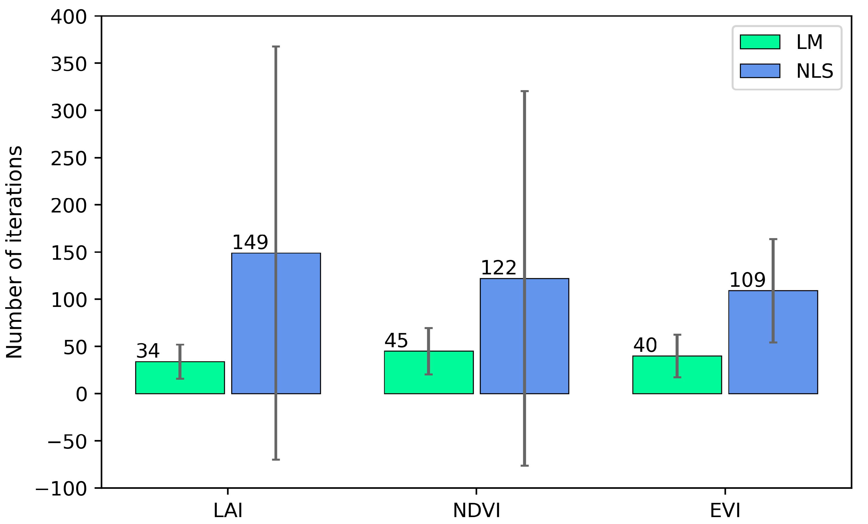
Nonlinear model fitting for large datasets requires speedy convergence indicated by the minimum number of iterations for the model to converge at each pixel. We used three satellite-based datasets (LAI, NDVI, and EVI) to compare the convergence efficiency of the two nonlinear fitting methods by fitting a double-logistic model and found that the LM method converged much faster than the NLS method for all the three datasets in our test area (Figure 1). The average convergence speed of all the pixels in the test area for the LAI dataset was 34 iterations/pixel for the LM method, while the average convergence speed for the NLS method was 149 iterations/pixel. The average convergence speed for the NDVI dataset was 45 and 122 iterations/pixel for the LM and NLS method, respectively. For the EVI dataset the convergence speed was 40 and 109 iterations/pixel, respectively, for the two methods (Figure 1).

Figure 1.
The average number of iterations and its spatial variation in fitting a double-logistic model using the LM and NLS method.
In addition to the average number of iterations, we also compared the two methods in terms of the spatial variation of convergence iterations. We found that the LM method had a much smaller spatial variation than the NLS method (Figure 1), suggesting the LM method is more stable in fitting double-logistic equations for different pixels across our test area.
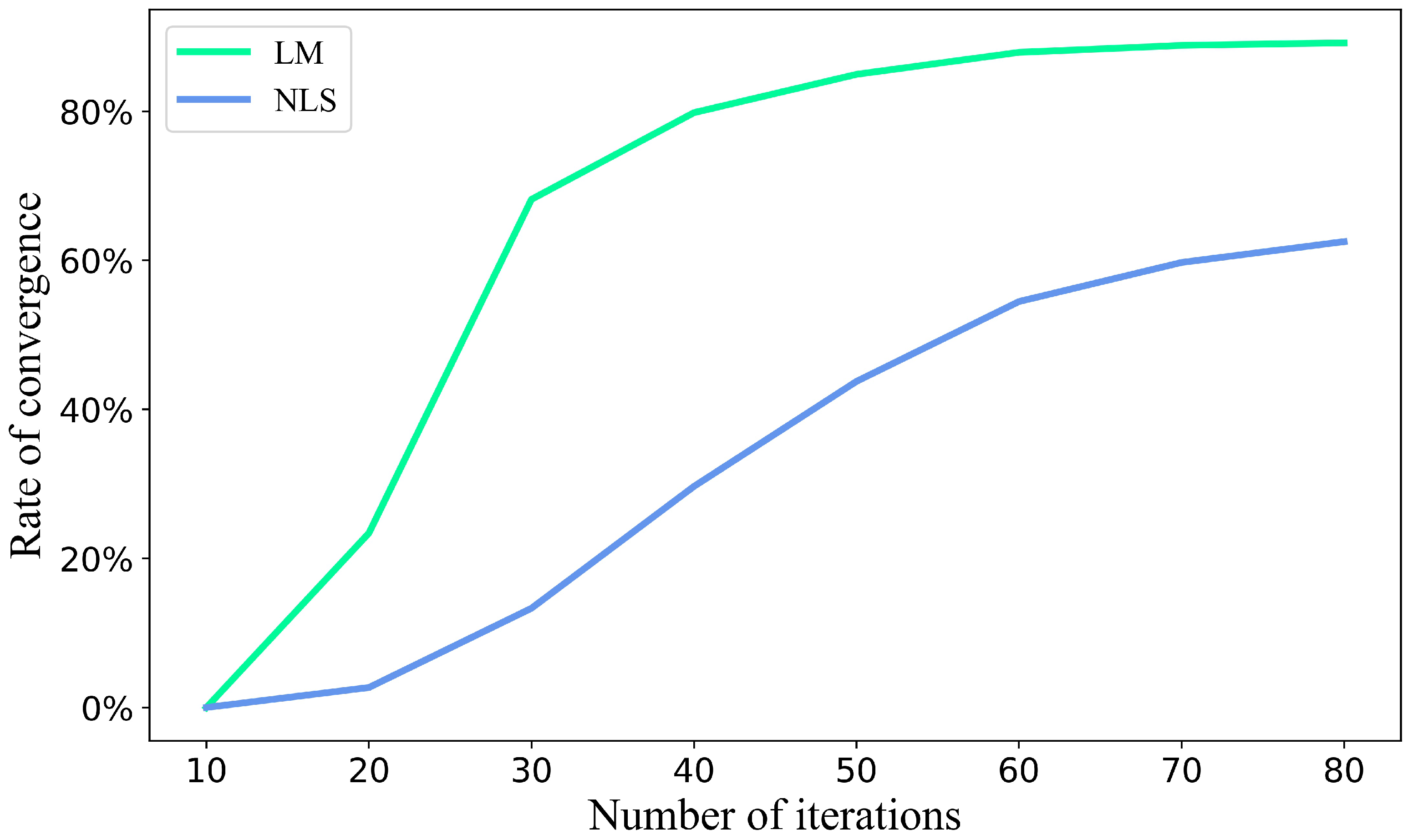
Nonconvergence is often seen in nonlinear model fitting, which is also related to the fitting method in addition to the characteristics of the data. We used a satellite-based LAI dataset to compare the rate of convergence, the number of pixels converged divided by the total number of pixels in the test area, of the LM and NLS methods by fitting double-logistic models for more than 21,318 pixels in our test area as mentioned earlier. We found that the rate of convergence increased nonlinearly with the increase of iterations (Figure 2). We also found that the LM method had a greater convergence rate than the NLS method. The convergence rate reached about 90% for the LM method when the number of iterations approached 80, while the convergence rate was barely 65% with the same number of iterations using the NSL method (Figure 2).
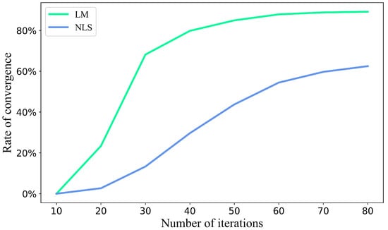
Figure 2.
Comparison of the convergence rates of the LM and NSL methods in fitting double-logistic models under different number of iterations.
3.2. Effects of Initial Values on Fitting the Double-Logistic Models
The initial value is an important factor affecting the convergence of nonlinear model fitting in addition to the fitted result. We designated 27 sets of different initial values to compare the two nonlinear fitting methods by fitting double-logistic models. We found that the fitted parameters were very similar for both methods when the models were convergent. We found, however, that the percentage of convergence in our test area was very different between the two methods. The LM method was much less sensitive to initial values than the NLS method (Table 1). The convergence rate of the LM method ranged from 67.4% to 92.1% with an average convergence rate of 86.2% for the 27 sets of initial values. Meanwhile, the convergence rate of the NLS method ranged from 6.7% to 59.1% with an average value of 35.4% for the same sets of initial values.

Table 1.
Convergence rate of fitting double-logistic equations with different initial values.
3.3. Comparison of the Results of the GEE-Based LM Method with Those of the Python-Based LM Method
We compared the results of our GEE-based LM method with those of the Python-based method by fitting the MODIS LAI data in our test area as defined earlier. We found that the results of the GEE and Python platforms were almost identical for each pixel in our test area (Table 2). For the six parameters of the DL model, the minimum, maximum, and median value of each parameter in the test area was identical to the fourth decimal point except parameter , which had a larger difference, 9.830209 versus 10.381544 for the Python and GEE platforms, respectively, (Table 2). The mean value of each parameter over the whole test area was slightly different between the two platforms with a difference of less than 2.07%. The p-values (0.0) from a paired t-test with 205 samples (pixels) was not statistically significant.
Table 2.
Statistics of the parameters of the double-logistic equations fitted with MODIS annual LAI data by the Python and GEE platform in the test area.
3.4. Implementation of the LM Method on the GEE Platform
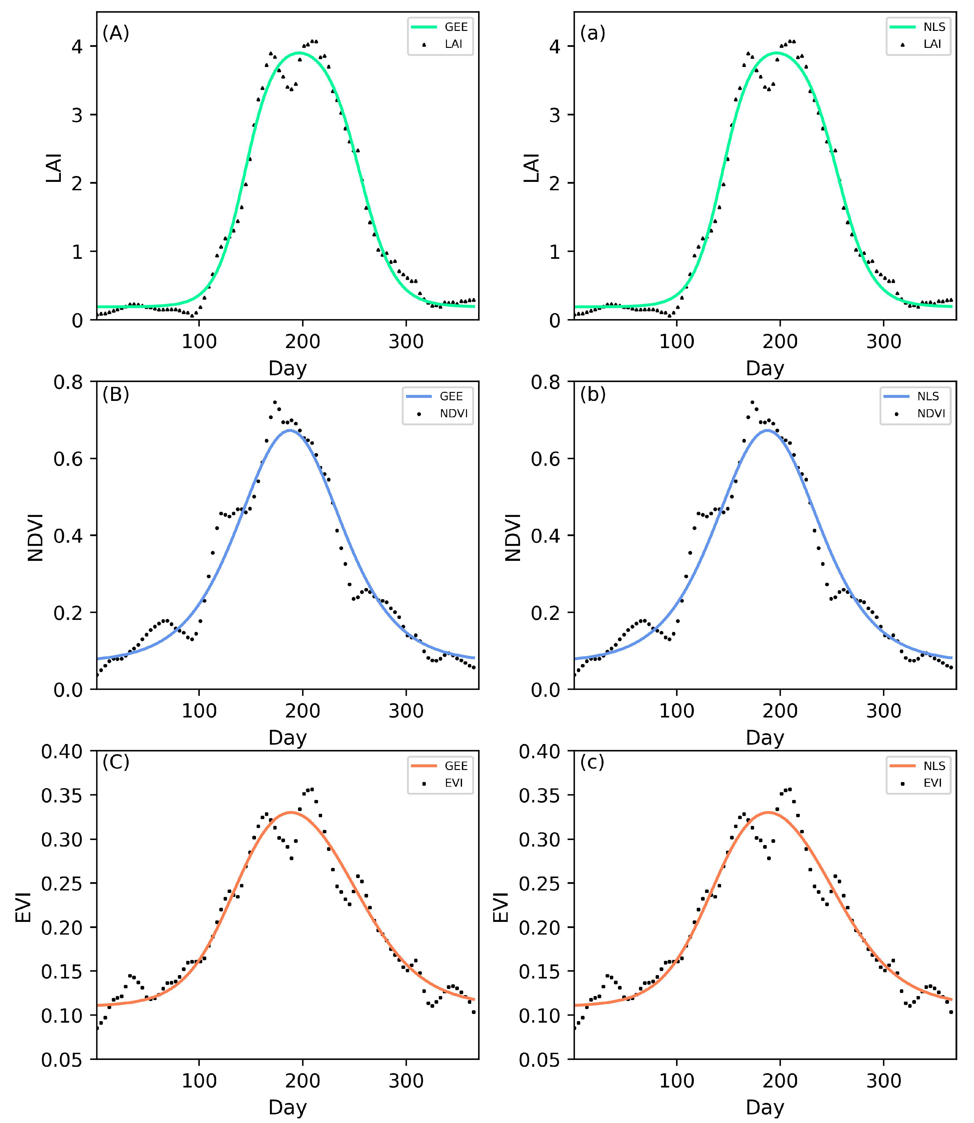
As we demonstrated that the LM method was superior to the NLS method in terms of convergence speed and initial value sensitivity, we implemented the LM method on the GEE platform by developing a new application. This application can be used to fit any nonlinear models with the GEE platform, and it is open to the public for free and available at https://figshare.com/s/34e7abe8c04ee66a19f7 (accessed on 20 April 2022). For demonstration purpose, we used three satellite-based datasets (LAI, NDVI, and EVI) to compare the fitting results of the two nonlinear methods by fitting double-logistic models and found that the results of the GEE-based LM method and NLS method were almost identical on the GEE platform for each pixel in our test area. Figure 3 shows the fitting results of one of the pixels. As expected, the models were well fitted to represent the seasonal trends of the variables (Figure 3). The flowchart for implementing the LM parallel algorithm on the GEE platform is given in Appendix A and the flow Algorithm A1 in Appendix B.
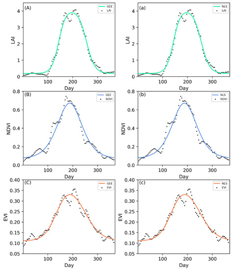
Figure 3.
Comparison of the observations and fitting equation by the GEE-based LM method and NLS method.(Fitting the double logistic model using the LAI data on the GEE platform (A) and the NLS method (a),using the NDVI data on the GEE platform (B) and the NLS method (b),using the EVI data on the GEE platform (C) and the NLS method (c)).
4. Discussion
4.1. Advantages of the LM Method
The LM method adaptively varies the parameter updates between the gradient descent update and the Gauss–Newton update. The LM method begins with the steepest descent to take benefit of its low sensitivity toward initial values. The Gauss–Newton method uses a Jacobian matrix to approximate Newton’s method’s Hessian matrix, which improves the efficiency of convergence. The LM method uses the trust region radius to prevent the Gauss–Newton method Jacobian matrix from being singular. Automatic switching of the steepest descent to Gauss–Newton within the LM method is ensured by the trust region radius.
In this study, we found that the LM method was superior to the NLS method in fitting nonlinear models with remote sensing data on the GEE platform. The LM method converged faster and was less sensitive to initial values than the NLS method. In addition, the LM method also had a much greater convergence rate in our test area. This method has also been successfully used to fit nonlinear models in different fields. For example, Dkhichi et al. (2014) [43] found that the LM method could improve model fitting accuracy with a solar cell model. Franchois et al. (1997) [44] found that including the LM method into a 2D complex permittivity reconstruction model could considerably improve the model performance in reconstructing circular geometry around an object. Transtrum et al. (2012) [26] improved the LM method by accepting uphill steps and employing the Broyden method to update the Jacobian matrix. This improvement can reduce the number of iterations, but it increases the computational cost of the residual on the shift , which might not improve the overall computation efficiency. Ahearnetal et al. (2015) [45] compared the LM method with the MINPACK-1 method using multiple initial values and found that the MINPACK-1 method generally outperformed the LM method to find the global optimal using a small physiological dataset. For fitting long-time series remote sensing data at a global scale, the MINPACK-1 method with multiple initial values is not feasible due to gigantic demands of computation resources.
4.2. Advantages of the GEE Platform
Google Earth Engine (GEE) is a cloud-computing platform strengthened for geospatial analysis and contains a large amount of publicly available imageries and other types of datasets [4,46,47,48,49,50]. Li et al. (2019) characterized the long-term mean seasonal pattern of phenology indicators of the start of season (SOS) and the end of season (EOS), fitting linearized double-logistic model using a statistics approach on the GEE platform [5]. However, the LM method we implemented on the GEE platform only needs to give the initial values to fit any nonlinear model. The linearization of nonlinear models requires a high level of mathematics, and not all nonlinear models can be linearized; thus, many studies cannot be carried out on the GEE platform at present. Yang et al. (2019) segmented the NDVI data into several adjacent segments according to the key temporal points and fitted the double-logistic model using the observed data points in each segment with serial computing to reconstruct the NDVI time series data without cloud points or gaps [51]. However, the LM method we implemented on the GEE platform fitted nonlinear model in parallel to save time and improve computational efficiency. We fitted any nonlinear model on the GEE platform by using the LM method, expanding the research field of GEE using Python and JavaScript programs. With the help of the JavaScript API and Python API, one can easily access and analyze geospatial datasets using various methods on Google’s cloud computing and processing platform, which provides a convenient development environment. Moreover, parallel computing on the GEE platform greatly boosts the speed of data processing and model fitting, especially with large datasets.
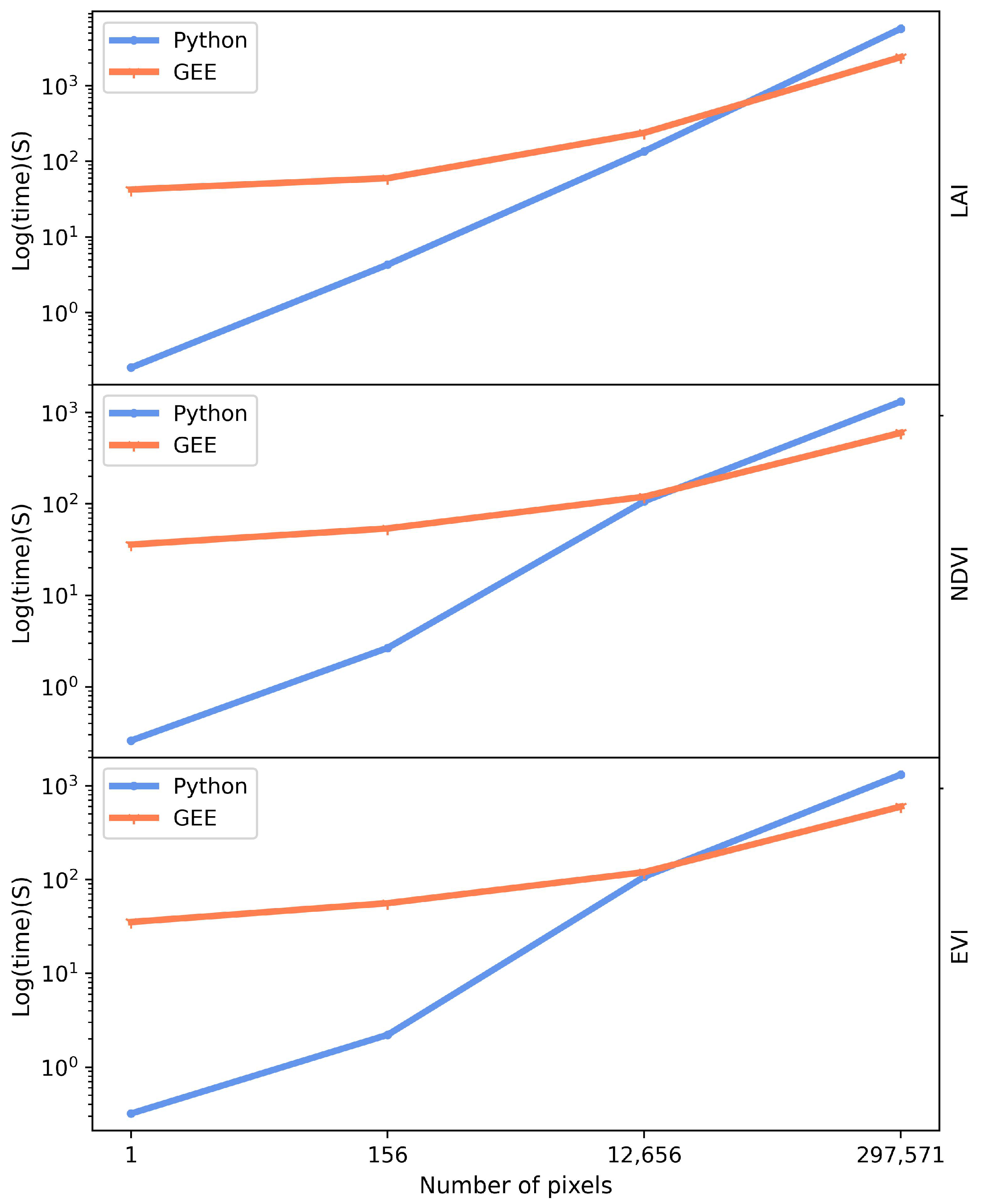
In the current study, we developed a new nonlinear fitting tool for the GEE platform and tested it using three satellite-based datasets (LAI, NDVI, and EVI). We also compared this GEE-based tool with a Python-based LM tool, a widely used program on personal computers and workstations. We found that the GEE-based tool was slower than the Python-based algorithm when the number of pixels was under about 13,000, but the GEE platform was much faster than the Python program when the number of pixels exceeded 13,000 (Figure 4). However, the current LM method can only iterate 80 times on the GEE platform due to resources limitation. The program returns a value of 0 for all the parameters if the equation does not converge after 80 iterations. In this case, the users can save the parameters and use these parameters as the initial values for the next run of the program to increase the total number of iterations. However, we found that increasing the number of iterations had little effect on improving the convergence for the three MODIS datasets (LAI, EVI, NDVI), suggesting that 80 iterations were enough for most applications with remote sensing data. We examined the results and found that low quality or missing remote sensing data caused the failure to converge, therefore, cleaning the datasets, by means such as removing low quality data or filling missing data before fitting the models, is necessary.
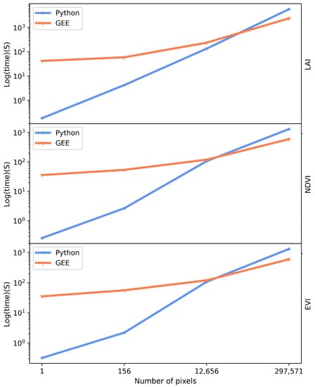
Figure 4.
Comparison of the execution time of the Python and GEE platforms in fitting double-logistic models with a different number of pixels by using data from LAI, NDVI, EVI.
5. Conclusions
We compared the Levenberg–Marquardt (LM) and nonlinear least square (NLS) methods in terms of convergence speed and initial value stability. We found that the LM method had a faster convergence rate, and it was insensitive to the initial values. We evaluated the accuracy of fitting the DL equations on the GEE platform using the LM method. The precision of fitting the DL equation by GEE-LM methods was around 0.0001, which satisfies the requirements of most applications. In addition to the remote sensing datasets, this nonlinear fitting tool can also be used to fit nonlinear models for other types of data, such as climate, vegetation, soil, and socioeconomic data.
The current LM method can only iterate 80 times on the GEE platform due to resources limitation. The program returns a value of 0 for all the parameters if the equation does not converge after 80 iterations. In this case, the users can save the parameters and use these parameters as the initial values for the next run of the program to increase the total number of iterations. However, we found that increasing the number of iterations had little effect on improving the convergence for the three MODIS datasets (LAI, EVI, NDVI), suggesting that 80 iterations were enough for most applications with remote sensing data. We examined the results and found that data quality, such as missing data and outliers, was mainly responsible for the failure to converge.
For future studies we plan to further improve the convergence rate by removing outliers and filling missing data before fitting the nonlinear models. We also plan to further improve the LM method by reducing the computational complexity to speed up convergence.
Author Contributions
Conceptualization, M.X.; methodology, M.X., S.W. and X.Z.; software, M.X., S.W. and X.Z.; validation, M.X., S.W. and X.Z.; formal analysis, S.W. and X.Z.; investigation, M.X. and Y.W.; data curation, S.W., X.Z. and Y.W.; writing—original draft preparation, M.X., S.W. and X.Z.; writing—review and editing, M.X., S.W. and X.Z.; supervision, M.X.; project administration, M.X.; funding acquisition, M.X. All authors worked together to design this work and have read and agreed to the published version of the manuscript.
Funding
This research was supported by the National Key Research and Development Program of China (2017YFA0604302, 2018YFA0606500).
Data Availability Statement
The data (LAI) presented in this study are available online: https://doi.org/10.5067/MODIS/MCD15A3H.061 and The data (NDVI, EVI) presented in this study are available online: https://doi.org/10.5067/MODIS/MOD13Q1.006. The LM method on the GEE platform we implemented can be fit any nonlinear models, and it is open to public for free and available at https://figshare.com/s/34e7abe8c04ee66a19f7.
Conflicts of Interest
The authors declare no conflict of interest.
Appendix A. Flowchart of the Levenberg–Marquardt Parallel Method
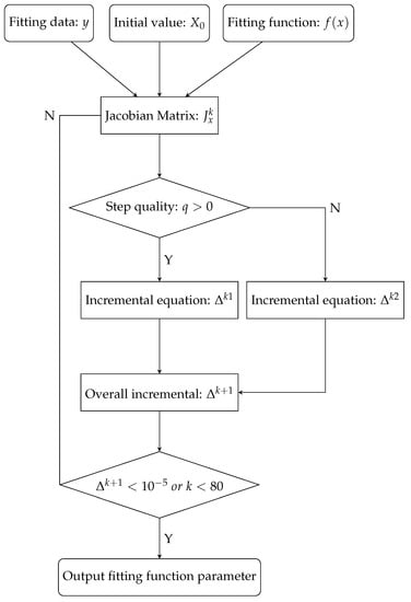
Figure A1.
Flowchart of the Levenberg–Marquardt Parallel Method.
Figure A1.
Flowchart of the Levenberg–Marquardt Parallel Method.

Appendix B. Flow of the Levenberg–Marquardt Parallel Method
| Algorithm A1 Flow of the Levenberg–Marquardt parallel method. |
| Require:
while do end while |
References
- Yuan, Y.-X. Trust Region Algorithms for Nonlinear Equations; Department of Mathematics, Hong Kong Baptist University: Hong Kong, 1994. [Google Scholar]
- Fan, J. Convergence Rate of The Trust Region Method for Nonlinear Equations Under Local Error Bound Condition. Comput. Optim. Appl. 2006, 2, 215–227. [Google Scholar] [CrossRef]
- Colson, B.; Marcotte, P.; Savard, G. A trust-region method for nonlinear bilevel programming: Algorithm and computational experience. Comput. Optim. Appl. 2005, 2, 211–227. [Google Scholar] [CrossRef] [Green Version]
- Gorelick, N.; Hancher, M.; Dixon, M.; Ilyushchenko, S.; Thau, D.; Moore, R. Google Earth Engine: Planetary-scale geospatial analysis for everyone. Remote Sens. Environ. 2017, 2, 18–27. [Google Scholar] [CrossRef]
- Li, X.; Zhou, Y.; Meng, L.; Asrar, G.R.; Lu, C.; Wu, Q. A dataset of 30m annual vegetation phenology indicators (1985–2015) in urban areas of the conterminous United States. Earth Syst. Sci. Data 2019, 2, 881–894. [Google Scholar] [CrossRef] [Green Version]
- Descals, A.; Verger, A.; Yin, G.; Peñuelas, J. A threshold method for robust and fast estimation of land-surface phenology using google earth engine. IEEE J. Sel. Top. Appl. Earth Obs. Remote Sens. 2020, 2, 601–606. [Google Scholar] [CrossRef]
- Kennedy, R.; Yang, Z.; Gorelick, N.; Braaten, J.; Cavalcante, L.; Cohen, W.; Healey, S. Implementation of the LandTrendr Algorithm on Google Earth Engine. Remote Sens. 2018, 10, 691. [Google Scholar] [CrossRef] [Green Version]
- Eythorsson, D.; Gardarsson, S.M.; Ahmad, S.K.; Hossain, F.; Nijssen, B. Arctic climate and snow cover trends–Comparing global circulation models with remote sensing observations. Int. J. Appl. Earth Obs. Geoinf. 2019, 2, 71–81. [Google Scholar] [CrossRef]
- Zeng, H.; Wu, B.; Zhang, N.; Tian, F.; Phiri, E.; Musakwa, W.; Zhang, M.; Zhu, L.; Mashonjowa, E. Spatiotemporal Analysis of Precipitation in the Sparsely Gauged Zambezi River Basin Using Remote Sensing and Google Earth Engine. Remote Sens. 2019, 2, 2977. [Google Scholar] [CrossRef] [Green Version]
- Wang, Y.; Ziv, G.; Adami, M.; Mitchard, E.; Batterman, S.A.; Buermann, W.; Marimon, B.S.; Junior, B.H.M.; Reis, S.M.; Rodrigues, D.; et al. Mapping tropical disturbed forests using multi-decadal 30 m optical satellite imagery. Remote Sens. Environ. 2019, 2, 474–488. [Google Scholar] [CrossRef]
- Papaiordanidis, S.; Gitas, I. Soil erosion prediction using the Revised Universal Soil Loss Equation (RUSLE) in Google Earth Engine (GEE) cloud-based platform. Bull. Soil Res. Inst. 2019, 100, 36–52. [Google Scholar] [CrossRef]
- Assefa, S.; Kessler, A.; Fleskens, L.J.S. Assessing Farmers’ Willingness to Participate in Campaign-Based Watershed Management: Experiences from Boset District, Ethiopia. Sustainability 2018, 2, 4460. [Google Scholar] [CrossRef] [Green Version]
- Marquardt, D.W. An algorithm for least-squares estimation of nonlinear parameters. J. Soc. Ind. Appl. Math. 1963, 2, 431–441. [Google Scholar] [CrossRef]
- Gill, P.E.; Murray, W. Algorithms for the solution of the nonlinear least-squares problem. SIAM J. Numer. Anal. 1978, 2, 977–992. [Google Scholar] [CrossRef]
- Dennis, J.E., Jr.; Gay, D.M.; Walsh, R.E. An adaptive nonlinear least-squares algorithm. ACM Trans. Math. Softw. (TOMS) 1981, 2, 348–368. [Google Scholar] [CrossRef]
- Curry, H.B. The method of steepest descent for non-linear minimization problems. Q. Appl. Math. 1944, 2, 258–261. [Google Scholar] [CrossRef] [Green Version]
- Fliege, J.; Svaiter, B.F. Steepest descent methods for multicriteria optimization. Math. Methods Oper. Res. 2000, 2, 479–494. [Google Scholar] [CrossRef]
- Battiti, R. First-and second-order methods for learning: Between steepest descent and Newton’s method. Neural Comput. 1992, 2, 141–166. [Google Scholar] [CrossRef]
- Yuan, Y.X. A new stepsize for the steepest descent method. J. Comput. Math. 2006, 24, 149–156. [Google Scholar]
- Lin, C.-J.; Weng, R.C.; Keerthi, S.S. Trust region newton method for logistic regression. J. Mach. Learn. Res. 2008, 2, 627–650. [Google Scholar]
- Deuflhard, P. A modified Newton method for the solution of ill-conditioned systems of nonlinear equations with application to multiple shooting. Numer. Math. 1974, 2, 289–315. [Google Scholar] [CrossRef]
- Deuflhard, P. Global inexact Newton methods for very large scale nonlinear problems. IMPACT Comput. Sci. Eng. 1991, 2, 366–393. [Google Scholar] [CrossRef]
- Hartley, H.O. The modified Gauss–Newton method for the fitting of non-linear regression functions by least squares. Technometrics 1961, 2, 269–280. [Google Scholar] [CrossRef]
- Gratton, S.; Lawless, A.S.; Nichols, N.K. Approximate Gauss–Newton methods for nonlinear least squares problems. SIAM J. Optim. 2007, 2, 106–132. [Google Scholar] [CrossRef] [Green Version]
- Chen, J. The convergence analysis of inexact Gauss–Newton methods for nonlinear problems. Comput. Optim. Appl. 2008, 2, 97–118. [Google Scholar] [CrossRef]
- Transtrum, M.K.; Sethna, J.P. Improvements to the Levenberg–Marquardt algorithm for nonlinear least-squares minimization. arXiv 2012, arXiv:1201.5885. [Google Scholar]
- Pujol, J.J.G. The solution of nonlinear inverse problems and the Levenberg–Marquardt method. Geophysics 2007, 72, W1–W16. [Google Scholar] [CrossRef]
- Moré, J.J. The Levenberg–Marquardt algorithm: Implementation and theory. In Numerical Analysis; Springer: Berlin/Heidelberg, Germany, 1978; pp. 105–116. [Google Scholar]
- Ma, C.; Jiang, L. Some research on Levenberg–Marquardt method for the nonlinear equations. Appl. Math. Comput. 2007, 2, 1032–1040. [Google Scholar] [CrossRef]
- Fan, J.-Y. A modified Levenberg–Marquardt method for singular system of nonlinear equations. J. Comput. Math. 2003, 2, 625–636. [Google Scholar]
- Fan, J.-Y.; Yuan, Y.-X. On the Quadratic Convergence of the Levenberg–Marquardt Method without Nonsingularity Assumption. Computing 2005, 2, 23–39. [Google Scholar] [CrossRef]
- Roweis, S.J.N. Levenberg-marquardt optimization. In Notes; University of Toronto: Toronto, ON, Canada, 1996. [Google Scholar]
- Ranganathan, A. The levenberg-marquardt algorithm. Tutoral LM Algorithm 2004, 11, 101–110. [Google Scholar]
- Madsen, K.; Nielsen, H.B.; Tingleff, O. Methods for Non-Linear Least Squares Problems. 2004. Available online: https://orbit.dtu.dk/files/2721358/imm3215.pdf (accessed on 2 April 2004).
- Fisher, J.; Mustard, J.; Vadeboncoeur, M. Green leaf phenology at Landsat resolution: Scaling from the field to the satellite. Remote Sens. Environ. 2006, 2, 265–279. [Google Scholar] [CrossRef]
- Elmore, A.J.; Guinn, S.M.; Minsley, B.J.; Richardson, A.D. Landscape controls on the timing of spring, autumn, and growing season length in mid-Atlantic forests. Glob. Chang. Biol. 2012, 2, 656–674. [Google Scholar] [CrossRef] [Green Version]
- Zeng, L.; Wardlow, B.D.; Xiang, D.; Hu, S.; Li, D. A review of vegetation phenological metrics extraction using time-series, multispectral satellite data. Remote Sens. Environ. 2020, 237, 111511. [Google Scholar] [CrossRef]
- Moglich, A. An open-source, cross-platform resource for nonlinear least-squares curve fitting. ACS Publ. 2018, 2, 2273–2278. [Google Scholar] [CrossRef]
- Oliphant, T.E. SciPy Tutorial. 2004. Available online: http://mat.fsv.cvut.cz/aznm/Documentation.pdf (accessed on 8 October 2004).
- Turley, R.S. Fitting ALS Reflectance Data Using Python. Faculty Publications. 2018. Available online: https://scholarsarchive.byu.edu/facpub/2099/ (accessed on 12 May 2018).
- Myneni, R.; Knyazikhin, Y.; Park, T. MCD15A3H MODIS/Terra+ aqua leaf area index/FPAR 4-day L4 global 500m SIN grid V006 [Data Set]. NASA EOSDIS Land Processes DAAC. 2015. Available online: https://lpdaac.usgs.gov/products/mcd15a3hv061/ (accessed on 11 October 2013).
- Didan, K. MOD13Q1 MODIS/Terra Vegetation Indices 16-Day L3 Global 250m SIN Grid V006 [Data Set]. NASA EOSDIS Land Processes DAAC. 2015. Available online: https://lpdaac.usgs.gov/products/mod13q1v006/ (accessed on 11 October 2013).
- Dkhichi, F.; Oukarfi, B.; Fakkar, A.; Belbounaguia, N. Parameter identification of solar cell model using Levenberg–Marquardt algorithm combined with simulated annealing. Sol. Energy 2014, 2, 781–788. [Google Scholar] [CrossRef]
- Franchois, A.; Pichot, C. Microwave imaging-complex permittivity reconstruction with a Levenberg–Marquardt method. IEEE Trans. Antennas Propag. 1997, 2, 203–215. [Google Scholar] [CrossRef]
- Ahearn, T.S.; Staff, R.T.; Redpath, T.W.; Semple, S.I.K. The use of the Levenberg–Marquardt curve-fitting algorithm in pharmacokinetic modelling of DCE-MRI data. Phys. Med. Biol. 2005, 50, N85. [Google Scholar] [CrossRef]
- Amani, M.; Ghorbanian, A.; Ahmadi, S.A.; Kakooei, M.; Moghimi, A.; Mirmazloumi, S.M.; Moghaddam, S.H.A.; Mahdavi, S.; Ghahremanloo, M.; Parsian, S. Google earth engine cloud computing platform for remote sensing big data applications: A comprehensive review. IEEE J. Sel. Top. Appl. Earth Obs. Remote Sens. 2020, 2, 5326–5350. [Google Scholar] [CrossRef]
- Kumar, L.; Mutanga, O. Google Earth Engine Applications Since Inception: Usage, Trends, and Potential. Remote Sens. 2018, 10, 1509. [Google Scholar] [CrossRef] [Green Version]
- Moore, R.; Hansen, M. Google Earth Engine: A new cloud-computing platform for global-scale earth observation data and analysis. In Proceedings of the AGU Fall Meeting Abstracts, San Francisco, CA, USA, 5–9 December 2011. IN43C-02. [Google Scholar]
- Mutanga, O.; Kumar, L. Google earth engine applications. Remote Sens. 2019, 11, 591. [Google Scholar] [CrossRef] [Green Version]
- Tamiminia, H.; Salehi, B.; Mahdianpari, M.; Quackenbush, L.; Adeli, S.; Brisco, B. Google Earth Engine for geo-big data applications: A meta-analysis and systematic review. ISPRS J. Photogramm. Remote Sens. 2020, 2, 152–170. [Google Scholar] [CrossRef]
- Yang, Y.; Luo, J.; Huang, Q.; Wu, W.; Sun, Y. Weighted double-logistic function fitting method for reconstructing the high-quality sentinel-2 NDVI time series data set. Remote Sens. 2019, 2, 2342. [Google Scholar] [CrossRef] [Green Version]
Publisher’s Note: MDPI stays neutral with regard to jurisdictional claims in published maps and institutional affiliations. |
© 2022 by the authors. Licensee MDPI, Basel, Switzerland. This article is an open access article distributed under the terms and conditions of the Creative Commons Attribution (CC BY) license (https://creativecommons.org/licenses/by/4.0/).