Abstract
As clean, renewable energy, photovoltaic (PV) energy can reduce the ozone-layer loss and climate deterioration caused by the use of traditional types of energy to generate electricity. At present, most PV energy products involve the influence of cloud cover on solar radiation. However, the resolution and precision of most cloud cover data are not fine enough to reflect the actual cloud distribution in local areas. This leads to incorrect distribution results of PV energy in areas with high-spatial-variability clouds. Using high-resolution and high-precision cloud cover data obtained by satellite remote sensing to estimate the distribution of PV energy can solve this problem. In this study, the Global Land High-Resolution Cloud Climatology (GLHCC), a 10-day cloud frequency product with a resolution of 1 km and located in China, was used to construct a cloud-based solar radiation estimation model. Using the inverse relationship between cloud cover and solar radiation, the GLHCC was converted into sunshine percentage data. Using meteorological station data in China, a Least Squares Fit (LSF) and error check were carried out on the A-P, Lqbal, Bahel and Sen Models to determine the optimal solar radiation estimation model (Sen Model). Based on the sunshine percentage data, the Sen Model and terrain shielding factors, the distribution of PV energy in China was estimated. Finally, comparing to the Global Horizontal Irradiance (GHI) of the World Bank and the yearly average global irradiance of the Photovoltaic Geographic Information System (PVGIS), PV energy data in this paper more accurately reflected the distribution of PV energy in China, especially in areas with high-spatial-variability clouds.
1. Introduction
With the development of new energy (clean, renewable energy), the PV power generation output as a proportion of the total energy output has increased steadily [1,2]. After China proposed the concepts of “carbon neutral” and “peak carbon dioxide emissions” at the 75th Session of the United Nations General Assembly in 2020, the use of PV energy and other new energy has received increased attention [3]. As a renewable, clean energy, PV energy, through its use, can reduce the ozone-layer depletion and climate degradation caused by traditional energy use in electricity generation [4,5,6,7]. Therefore, PV power generation plays an important role in a country’s energy strategy. In the implementation of specific PV power generation strategies, without considering the influence of PV facilities, the choice of the PV power station location has a direct impact on the cost of power generation and determines the power output of PV energy.
The location of PV power stations is affected by many factors, including PV energy, terrain, traffic conditions and ground attachments [8,9]. The availability of PV energy is a prerequisite for the development value of a site. Due to the high cost of radiation measurement equipment, complex measurement technology and other factors, most meteorological stations lack radiation measurement conditions, and only the sunshine duration and other meteorological parameters are observed [10,11]. For example, China currently has 756 ground meteorological data observation stations open to the public, of which only 100 stations can observe solar radiation [12]. Compared with general meteorological data, such as temperature, cloud cover and sunshine duration, the distribution of meteorological stations used to observe solar radiation is generally sparse. This results in a lack of solar radiation data in most areas, which is difficult to meet the requirements of solar energy utilization and other applications. Therefore, it is a common choice of many solar radiation estimation models to estimate the distribution of PV energy using conventional meteorological data (temperature, cloud cover and sunshine duration).
Since Kimball [13] put forward the idea that there might be a strong correlation between sunshine percentage and total radiation in 1919, and Angstrom [14] devised the formula for total radiation in 1924, a large number of models for calculating total solar radiation have been established. These radiation models can be placed in three categories [15]: theoretical models [16], empirical models [17] and machine learning models [18]. The most commonly used theoretical models include the Hottel Model [19,20], Threlkeld and Jordan Model [19,21] and the ASHRAE Model [22,23]. Most theoretical models consider the influence of the main components of the atmosphere on the solar shortwave radiation in detail. The theoretical models have solid physical foundations, but their structures are extremely complex. The input parameters of the theoretical models include variables such as ozone-layer thickness, aerosol content and atmospheric precipitable water. These variables are difficult to obtain, which limits the popularization and application of theoretical models. A theoretical model is mainly used to calculate the solar radiation on sunny days and to represent the amount of solar radiation in the atmosphere under ideal conditions. However, due to the influence of the atmosphere, humidity, water vapor pressure and other factors, there are only a few days in a year when the amount of radiation is close to the solar radiation of a clear day. With the development of computer technology, in order to better deal with complex nonlinear problems, researchers have proposed many methods to estimate the radiation amount using machine learning models. These methods include the Artificial Neural Network (ANN) [24,25], Support Vector Machine (SVM) [26,27], Markov Model (MM) [28,29], Extreme Learning Machine (ELM) [30,31], Random Forest (RF) [32,33] and Gaussian Process Regression (GPR) models [34,35]. However, machine learning models are often characterized by high model complexity and long training times and are, therefore, not suitable for large-scale solar radiation estimation at the present stage. Empirical models use the correlation between solar radiation and other conventional meteorological parameters to construct a regression model to predict solar radiation. According to the meteorological factors that they use, the models are divided into sunshine percentage model [14,36,37,38,39,40], temperature model [41,42], cloud cover model [43,44] and component-decomposition model [45,46,47]. The high precision and simple form of an empirical model based on sunshine percentage mean that it is widely used [48,49,50,51].
Sunshine percentage is an important parameter for calculating the amount of solar radiation [36]. Usually, when simulating solar radiation, the observation data of sunshine duration at conventional meteorological stations are used. Such data have high reliability. However, the spatial continuity of meteorological stations is poor, and the distribution is irregular. In the past, the inverse distance weighting (IDW), Kriging, Spline Function and other interpolation methods were used to calculate the distribution of 1-D points on a 2-D plane. However, these methods do not consider the distribution characteristics of meteorological elements themselves, resulting in a large error in the estimation results. With the development of space technology in recent years, the data provided by satellites have high resolution in space and time, which makes up for the spatio-temporal dispersion of station data. It is of great significance to introduce the sunshine percentage generated using remote sensing data into the estimation of radiation.
The sunshine duration is usually determined by the amount of time the sun is obscured by sufficiently opaque clouds [52]. There is a marked inverse relationship between the sunshine duration and cloud cover, and according to Rangarajan [52], there is a linear relationship between total cloud cover and the sunshine percentage under ideal conditions. However, in practice, the estimation of cloud cover in a short time is not completely error-free and is affected by the observation angle and cloud movement. Although the relationship between the amount of cloud and sunshine percentage is not completely linear [53], the error is much reduced when using cloud cover data over a long enough period of time to estimate sunshine percentage. Therefore, based on the correlation between cloud cover and sunshine percentage, a cloud-based solar radiation estimation model can be established using cloud cover to produce continuous sunshine percentage data. At present, most PV energy products consider the influence of cloud cover on solar radiation, and some studies have tried to convert the amount of cloud into sunshine percentage [54,55,56]. However, the resolution of most cloud products is not fine enough to reflect the cloud distribution in local areas. The main satellite remote sensing cloud data include the National Oceanic and Atmospheric Administration (NOAA) series satellite cloud products [57,58], the International Satellite Cloud Climatology Project (ISCCP) products [59,60], the Earth Observing System (EOS) series satellite cloud products [61] and the Cloud Detecting Satellite (CloudSat) cloud products [62]. The spatial resolution of these products is greater than 3 km, which does not meet the research requirements of areas with high-spatial-variability clouds. Therefore, it is necessary to use a cloud product with high resolution and precision for generating sunshine percentage. Zhang et al. [63] produced the global land cloud coverage product GLHCC based on the 1 km MOD09 cloud mask from 2001 to 2016. The product has made two improvements to the MOD09 cloud mask, reducing the confusion between ice, snow, bright areas and clouds. GLHCC more accurately reflects global cloud distribution than PATMOS-X (Pathfinder Atmospheres—Extended) cloud products and long-term cloud frequency based on the MOD35 cloud mask. Therefore, GLHCC is a good choice for establishing a cloud-based solar radiation estimation model.
Therefore, this paper uses the 10-day cloud frequency product GLHCC in China with a resolution of 1 km to generate the sunshine percentage according to a linear model. The sunshine duration data and solar radiation data of 72 meteorological stations are used for the quarterly Least Squares Fit (LSF) to solve the best fitting coefficients of four models (A-P, Lqbal, Bahel and Sen Models). An error check is conducted on the fitting results of each model to select the most suitable PV energy estimation model for China. The quarterly coefficients and 10-day sunshine percentage generated by cloud cover are substituted into the optimal model to complete the preliminary prediction of the distribution of PV energy. The terrain shielding factor is calculated based on the principle of hillshade by using the real solar altitude angle and azimuth angle; the final PV energy distribution data are then obtained. The products in this study are produced in 10-day, monthly, quarterly and annual products for different applications. The annual distribution of PV energy in China provides an important reference for the location of PV power stations. The 10-day, monthly and quarterly products provide a reference for existing power stations to carry out peak regulation and energy storage and to supplement wind power generation or hydroelectric power generation at appropriate times. Finally, in order to prove that the GLHCC cloud product produces a more accurate result for the estimation of PV energy, we compare the PV product in this study with the Global Horizontal Irradiance (GHI) data and the irradiance data from the Photovoltaic Geographic Information System (PVGIS).
2. Study Area and Data
Since 2009, China has been vigorously developing the PV industry and implementing new energy strategies. Therefore, China is selected as the study area to study solar radiation estimation based on cloud cover. GLHCC cloud data, meteorological station data, Digital Terrain Elevation Model (DEM) data and related data for consistency checking are used in the specific experiment. The study area and the data used are described below.
2.1. Overview of the Study Area
China is located in the eastern part of Eurasia and the west coast of the Pacific Ocean, between 73°33′E–135°05′E and 3°51′N–53°33′N. China has various climate types, including a monsoon climate, a continental climate and a mountain climate. From the southeast coast to the northwest inland, the spatial distribution of annual precipitation shows a decreasing trend. In winter, due to the great distance between the north and south of China and the influence of the Siberian cold current, the north is very cold, while the south is not. In summer, high temperatures are widespread across the country due to the higher latitudes and longer days in the north, while the south is directly exposed to the sun. The terrain of China is high in the west and low in the east, with a ladder-like distribution. The mountains and plateaus cover a vast area, and the distance between east and west is about 5000 km, while the continental coastline is more than 18,000 km long.
China is a country with abundant solar energy resources, with more than two-thirds of its area having annual sunshine hours of more than 2000 h and annual radiation of more than 5000 . However, due to the differences in climate and terrain, the spatial heterogeneity of geographical factors is large. Therefore, solar energy resources are seriously unevenly distributed and have obvious spatial variation.
2.2. Data
2.2.1. GLHCC Global Land Cloud Coverage Products
The GLHCC is a high-resolution (1 km) and high-precision global land 10-day cloud frequency dataset [57]. GLHCC was derived from the MOD09 cloud mask from 1 January 2001 to 31 December 2016 and is provided as cloud mask flags in the MOD/MYD09GA daily surface reflectance product. This product uses a short wave, infrared threshold method and the B2/6 threshold method to improve and enhance the original MODIS (Moderate-resolution Imaging Spectroradiometer) cloud mask so as to reduce the confusion between ice and snow, bright areas and clouds. GLHCC cloud products are stored in a GeoTIFF format. The high resolution and high precision of the product readily meet the needs of a fine-grained model and the resolution requirements of PV power station locations in this study.
2.2.2. Meteorological Station Data
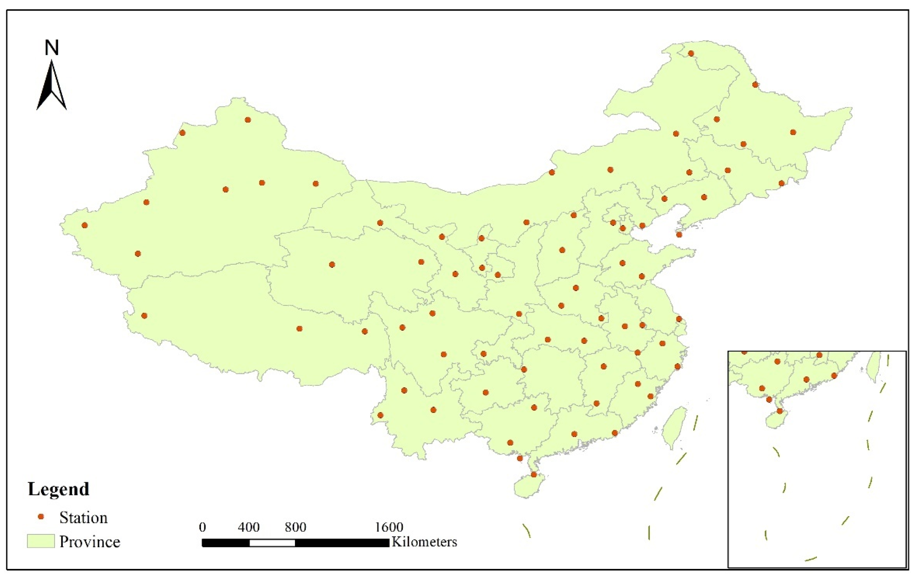
In this study, 100 stations providing sunshine duration and solar radiation data from the China Meteorological Administration (http://data.cma.cn (accessed on 8 September 2020)) were used, and the data from 72 high-quality stations were used as the standard data for the LSF for the solar radiation estimation models. The meteorological data of these stations is stored in a CSV format, and the stations are densely distributed in eastern China and sparsely distributed in western China, as shown in Figure 1.

Figure 1.
Distribution of solar radiation stations in China.
2.2.3. SRTM DEM Data
Shuttle Radar Topography Mission (SRTM) data were produced by the National Aeronautics and Space Administration (NASA), the National Image and Mapping Agency (NIMA) and the German and Italian space agencies. The interferometric imaging radar mounted on the US space shuttle “Endeavour” was used to obtain the radar data after 11 days of near-global operation. The dataset covers more than 80% of the global land surface with a uniform resolution and accuracy. The amount of radar image data obtained by the SRTM system is about 9.8 trillion bytes. After more than two years of data processing, a DEM is made; that is, the current SRTM terrain product data. The SRTM DEM has been used in various research fields to obtain many important scientific results. The SRTM products include grid data with spatial resolutions of 30 and 90 m, which are called “SRTM1” and “SRTM3”, respectively. The SRTM data used in this study are SRTM3.
2.2.4. Data for Consistency Checking
The data used for consistency checking in this study are the GHI data of the World Bank with a resolution of 250 m and the irradiance data from PVGIS with a resolution of 5 km.
Published studies by the World Bank provide the aggregated and unified views of solar energy resources, including PVOUT (Photovoltaic Power Potential), GHI (Global Horizontal Radiation), DIF (Diffuse Horizontal Radiation), GTI (Global Radiation for Optimal tilted Surfaces), OPTA (Optimal Tilt of Photovoltaic Modules), DNI (Direct Normal Exposure) and TEMP (Air Temperature, measured in °C). Solar energy, PV potential and other parameters are provided in the form of grid data in two formats: GeoTIFF and AAIGRID (ESRI ASCII grid). The GHI data used in this study are yearly average daily total solar radiation.
The irradiance data of PVGIS are calculated using the National Solar Radiation Database (NSRDB) [64], developed by the National Renewable Energy Laboratory (NREL). The NSRDB is a serially complete collection of hourly and half-hourly values of the three most common measurements of solar radiation—global horizontal, direct normal and diffuse horizontal irradiance—and meteorological data. The data available here are only long-term averages, calculated from hourly global and diffuse irradiance values over the period 2005–2015. The data are stored in the GeoTIFF format. The irradiance data used in this paper are the yearly average global irradiance on the horizontal plane from 2005 to 2015.
3. Materials and Methods
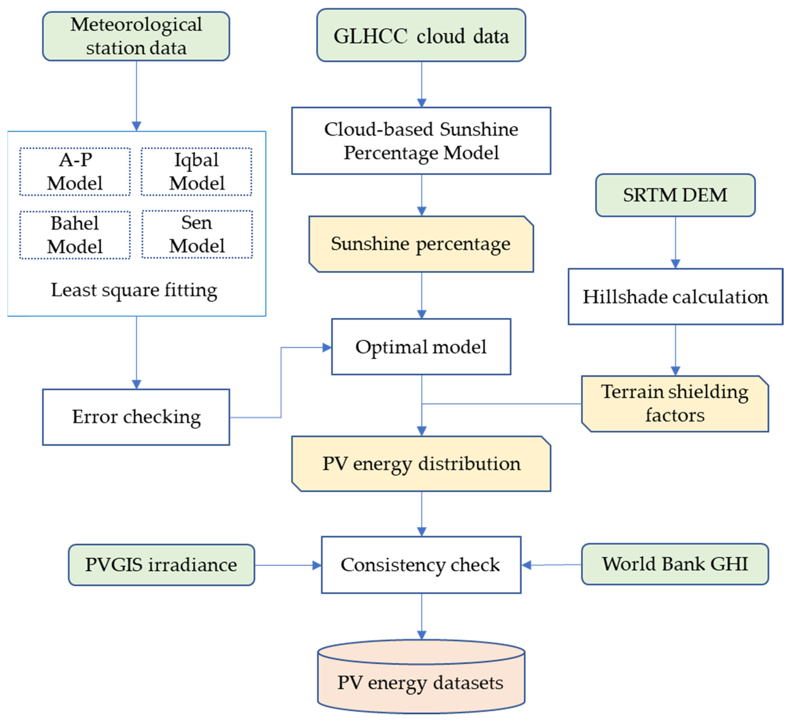
To build a cloud-based solar radiation estimation model, cloud cover is first converted into sunshine percentage data using a cloud-based sunshine percentage model. Then, using the meteorological station data and basic astronomical and geographical data, an LSF is carried out to solve the empirical coefficients of the A-P, Iqbal, Bahel and Sen Models. The most suitable solar radiation estimation model for China was determined by error-checking the fitting results of the four models. The SRTM DEM data were used to calculate the terrain shielding factor based on the hillshade calculation principle. Based on sunshine percentage data and the optimal model, the distribution of PV energy in China was estimated in combination with the terrain shielding. Finally, the GHI of the World Bank and the irradiance of PVGIS were used for consistency checking the PV products in this study. Figure 2 is a technical flowchart of the cloud-based solar radiation estimation model.

Figure 2.
Technical flowchart of the cloud-based solar radiation estimation model.
3.1. Relative Sunshine Percentage
In this study, the cloud frequency product GLHCC was used to generate the sunshine percentage according to the inverse relationship between cloud cover and solar radiation. The sunshine percentage here refers to the sunshine percentage with no error in cloud cover observations. The relationship between sunshine percentage and cloud cover is linear, as shown in Formula (1).
where is the total amount of cloud, which can also be said to be the cloud frequency; is the sunshine duration; and is the duration of possible sunshine.
There is a good negative correlation between total cloud cover and sunshine percentage, but the correlation differs significantly at different times. Therefore, when using cloud cover data to generate sunshine percentage, it should be integrated by period. In other words, the cloud cover data for period 36 generated the sunshine percentage data for period 36. The daily observational data for cloud cover, whether ground observation or satellite remote sensing data have a problem inherent to observation time; that is, the time term in a single day is discrete. Therefore, surplus data on a long time-series scale is used in this study to make up for the insufficient data on the single-day scale. The GLHCC is a 10-day product produced from 16 years of cloud observation data, which meets the requirements of this study. A long time-series average cloud frequency can better express a stable state of cloud cover in a time period, which is better for generating the sunshine percentage and for predicting the distribution of PV energy.
3.2. Calculation of Basic Astronomical and Geographic Data
Astronomical solar radiation (ASR), also known as extraterrestrial solar radiation and extra-atmospheric solar radiation, refers to the solar radiation when the sun reaches the upper boundary of the atmosphere. Its value is only related to the relative position of the sun and the earth and the geographical position of the earth’s surface. ASR forms not only the basic background of the amount of solar radiation received on the ground but is also one of the most important astronomical parameters in radiation calculation. The calculation formula of daily total ASR is given by Formula (2). In this study, the 10-day average daily total ASR was calculated using the daily total ASR.
where is the solar constant, which refers to the total radiation energy received from the sun per unit time per unit area on a theoretical surface perpendicular to the sun’s rays and at the earth’s mean distance from the sun. varies little from month to month, with an annual mean range of ±3.5%. For convenience of calculation, the annual average value of is taken, i.e.,:
is the eccentricity correction coefficient, which is given by Formula (4):
where is the day of the year from 1 January.
(solar declination) refers to the angle between the line joining the centers of the sun and the earth and its projection on the equatorial plane. is caused by the earth orbiting the sun at a certain inclination. Its value is only related to the calculated date, which varies from +2326′ to −2326′. The declination angle is given by Formula (5):
(hour angle) is the angle between an observer’s meridian (a great circle passing over his head and through the celestial poles) and the hour circle (any other great circle passing through the poles) on which some celestial body lies. The local hour angle at noon is 0, negative in the morning and positive in the afternoon, with a difference of every hour. (sunset angle) is calculated according to Formula (6):
where is the local latitude.
(duration of possible sunshine) is calculated using Formula (7):
3.3. Calculation of Empirical Coefficient of Radiation Estimation Model
The total solar radiation on the ground mainly depends on astronomical radiation and the weakening effect of the atmosphere on solar radiation. This weakening effect is expressed as the ratio of total solar radiation on the horizontal plane to astronomical radiation; that is, the clear sky index, as shown in Formula (8):
A large number of the literature and data studies show that there is a good correlation between the clear sky index and sunshine percentage. In 1924, Angstrom [14] proposed the earliest calculation model by using the correlation between the ratio of sunny solar radiation () to total radiation and the percentage of sunshine, as shown in Formula (9):
The application of Formula (9) is limited due to the complexity of the sunny solar radiation. In 1940, Prescott [32] modified Angstrom’s model and proposed to replace sunny solar radiation with astronomical radiation, as shown in Formula (10):
This model is called the A-P Model. The A-P Model provided a correlation between the clear sky index and sunshine percentage for the first time. The A-P Model is simple in form, and the calculation of astronomical radiation in the model is easy. Therefore, the A-P Model was quickly adopted by researchers and has become one of the most widely used models in solar radiation estimation.
Based on the A-P Model, subsequent researchers proposed models with quadratic polynomial, cubic polynomial, exponential and logarithmic forms.
Based on the meteorological data of three meteorological stations in Canada, Iqbal [33] proposed a quadratic polynomial model:
Based on the sunshine hours and total solar radiation data of 48 meteorological stations in different countries, Bahel [34] established a cubic polynomial model based on sunshine percentage, which is applicable to all countries:
Sen [65] proposed a simple three-coefficient nonlinear model to estimate global solar radiation from sunshine percentage:
This study intends to use the above four linear and nonlinear models to simulate the relationship between sunshine percentage and solar radiation in China and to calculate the optimal empirical coefficient of the models. The data of 72 stations with a continuous sunshine duration and solar radiation were selected and divided into four time periods according to season. The station data were substituted into the above four linear and nonlinear models to calculate the empirical coefficients of the radiation-estimation model. The empirical coefficient was solved using the LSF according to the linear model and nonlinear model. The LSF method calculates the optimal coefficient of the model by optimizing the sum of the squares of minimum error. The reason why the empirical coefficient was not calculated over 10 days is that an empirical coefficient arrived at using the data for 10 days out of 16 years does not guarantee its stability and the accuracy of the final result. Finally, empirical coefficients for models divided by season were obtained, which is suitable for the prediction of PV energy distribution every 10 days in this season.
3.4. Optimal Model Selection and Estimation of PV Energy Distribution
The accuracies of the four models with empirical coefficients are compared. The following three error checking formulas were used to analyze each model:
Determinable coefficient ():
Mean absolute error ():
Root mean square error ():
where, and are the simulation results and measured results, respectively, is the mean value of and n is the sample size.
The empirical coefficients of the best model were interpolated by IDW to obtain the empirical coefficients for each seasonal model throughout the country. The sunshine percentage integrated by the GLHCC and the basic astronomical and geographical data were substituted into the model to solve the preliminary distribution of PV energy per 10 days.
3.5. Calculation of Terrain Shielding Factor
When sunlight reaches the ground through clouds, it is affected by the local terrain, and the solar radiation reaching the ground is redistributed on the local surface. In areas with rugged terrain, due to the influence of terrain shielding, slope and slope direction, different slope surfaces receive different amounts of solar radiation [66]. Slope surfaces with a larger included angle with solar light receive more solar radiation. In contrast, slope surfaces with a smaller included angle with solar light have a relatively short direct exposure time and receive less solar radiation. A traditional solar radiation estimation model does not take into account the shielding of terrain against solar radiation, which should be considered one of the location factors of PV power stations. Several studies have considered the effect of terrain shielding on sunshine duration and solar radiation [67,68,69,70,71]. Since the placement angle of PV panels can be adjusted, this study only considers whether PV panels can receive sunlight at a certain time. Terrain shielding can be divided into direct radiation shielding and scattered radiation shielding. Direct radiation shielding mainly considers the incident angle between the sunlight and local terrain, while scattered radiation shielding considers the shielding of different conditions in each direction, which is necessary to build various anisotropic scattering radiation models. Therefore, this study only considers the influence of local terrain on the effects of direct radiation.
The calculation of the terrain shielding factor mainly considers the relationship among slope, slope direction, solar altitude angle and solar azimuth. As shown in Figure 3, the shielding area is divided into two main categories: One is the side of the mountain facing away from the sun, for which the slope is greater than the solar altitude; the other is the sheltered area that is blocked by the adjacent higher mountain and does not, therefore, receive sunlight. In order to study the shielding effect of local terrain on solar radiation, this study used DEM data with a resolution of 90 × 90 m to calculate slope, aspect and hillshade.
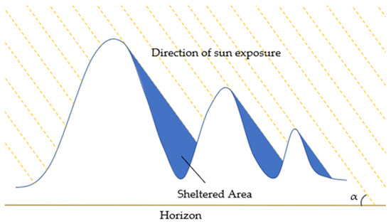
Figure 3.
Hillshade simulation diagram. The yellow dotted lines represents the direction of incident sunlight, the brown line represents the horizon and α represents the solar altitude.
The method of calculating the terrain shielding factor involves using the sunrise time as the starting point, the sunset time as the endpoint and 10 min as the time step to calculate the masking area within 10 min (binary image of 0 or 1). The sheltered areas were averaged to obtain the terrain shielding factor for a day (between 0 and 1); then, the daily terrain shielding factors were averaged every 10 days to obtain a 10-day terrain shielding factor, as shown in Formulas (17) and (18):
where is the sheltered area at time of day , is the terrain shielding factor of day and is the terrain-shielding factor within 10 days.
In this study, we used hillshade to calculate the sheltered area. The principle of a hillshade algorithm is to calculate the illuminance value of each pixel by setting the position of the assumed light source and using several adjacent pixels. If we set the real solar altitude and azimuth, we obtain the real terrain shadow. When the illumination value of a pixel is less than or equal to 0, it is part of a shadowed area, and the value of that pixel is set to 0; in contrast, in an area that receives sunlight, the value is set to 1, as shown in Formulas (19) and (20):
where is the hillshade, is the radian of the solar zenith angle and is the radian of the slope. is the radian of the solar azimuth and is the radian of the aspect in that area.
- Solar zenith angle
The solar zenith angle () refers to the included angle between the direction of incident light and the zenith (the direction perpendicular to the surface) and is the complement angle of the solar altitude angle (). Therefore, to calculate the solar zenith angle, we only need to calculate the solar altitude angle. The calculation formulas are the Formulas (21) and (22):
where is the radian of the latitude, is the radian of the solar declination and is the local hour angle.
- Solar azimuth angle
The solar azimuth angle is the azimuth angle of the Sun’s position. For solar energy applications, it is clockwise from due north, so east is , south is and west is . The angle is given by Formula (23):
- Calculation of slope and aspect
The slope is the degree of steepness and gentleness of the surface unit. Generally, the ratio of the vertical height h of the slope to the distance L in the horizontal direction is called the slope (or slope ratio). Aspect is the orientation of the slope, measured clockwise in degrees from 0 to , where 0 is north-facing, is east-facing, is south-facing and is west-facing. In a 3 × 3 window, the slope and aspect of each central pixel are calculated using the values of eight adjacent pixels of the pixel.
4. Results and Analysis
Based on sunshine percentage data and the Sen Model, and using terrain shielding, we successfully constructed a cloud-based solar radiation estimation model and obtained the estimation results of PV energy in China. Section 4.1 discussed the sunshine percentage data generated by cloud cover and seasonal variation. Section 4.2 presents the error-checking results for the four empirical models and the characteristics of the empirical coefficients. Section 4.3 describes the influence of terrain shielding on PV energy. Section 4.4 describes in detail the estimated results for PV energy in China and compares them with other solar radiation products.
4.1. Sunshine Percentage
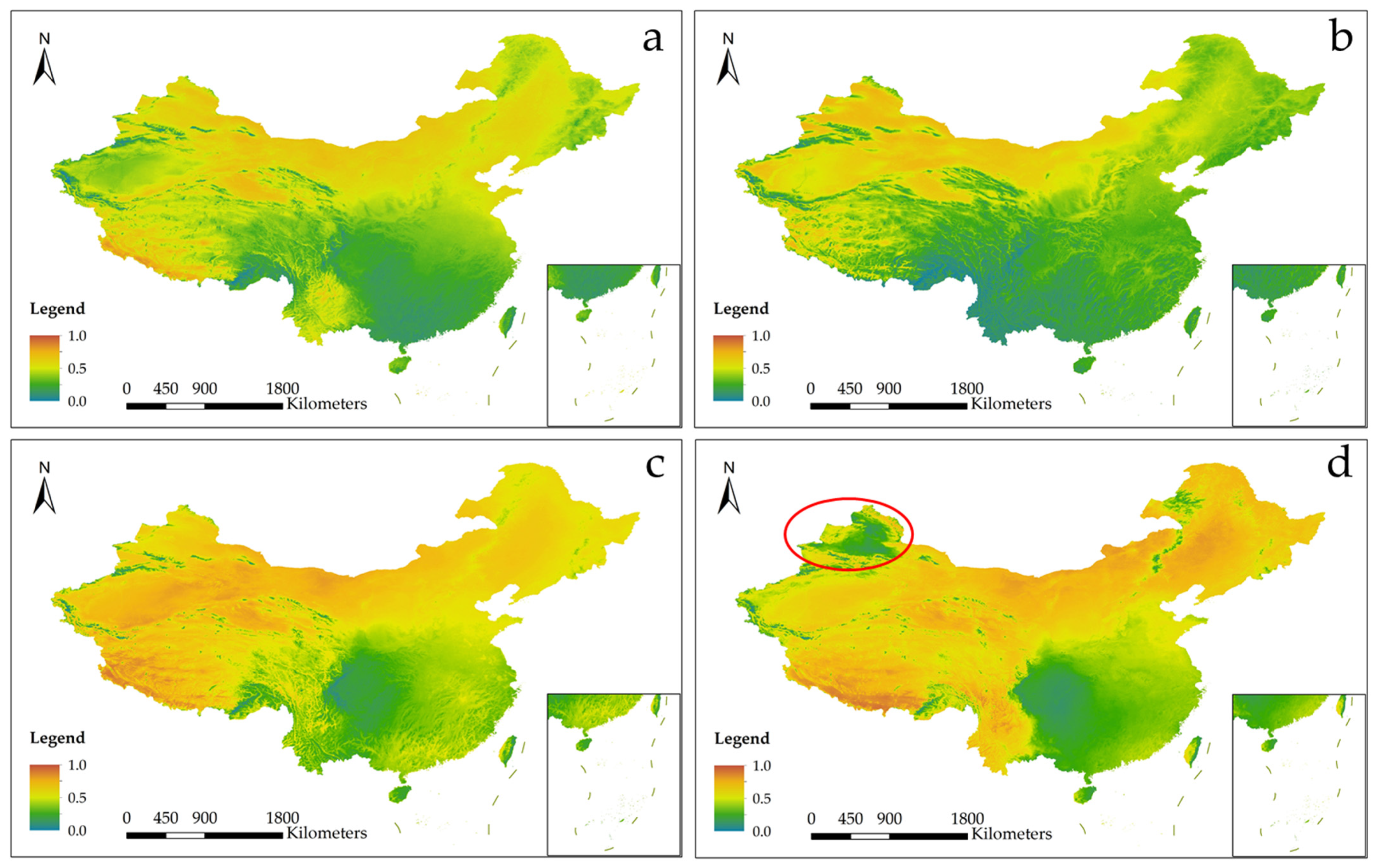
Figure 4 shows the average daily sunshine percentage for the four seasons based on cloud cover. Figure 4a shows the sunshine percentage in spring, which is obtained from the average sunshine percentage for every 10 days in March, April and May. Figure 4b shows the sunshine percentage in summer obtained from the average for June, July and August. Figure 4c shows the sunshine percentage in autumn obtained from the average for September, October and November. Figure 4d shows the sunshine percentage in winter obtained from the average for January, February and December. Figure 4 shows that, on the whole, the sunshine percentage is highest in winter and lowest in summer. The reason for this is that China has more precipitation in summer and less precipitation in winter. Regionally, the sunshine percentages in Xinjiang, Inner Mongolia, Northeast China and Qinghai Tibet Plateau are high, and the sunshine percentage in Sichuan Basin is low. This is because China has less precipitation in the north and more precipitation in the south. In high-altitude areas, the air is thin, and the rainfall is less. Figure 4d shows an unusual phenomenon: that is, the Junggar Basin in the northwestern corner of China (inside the red circle) shows a markedly low sunshine percentage. This is due to the unique cloudy and foggy weather formed by the unique terrain, humidity and temperature conditions in the Junggar Basin.
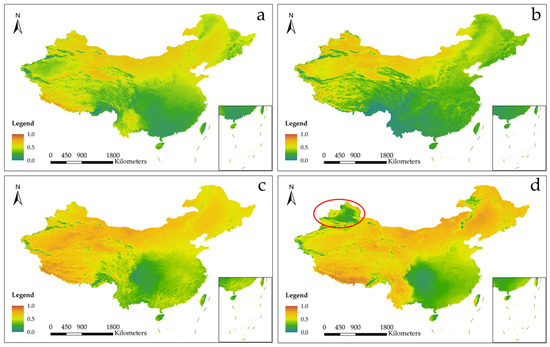
Figure 4.
Sunshine percentage based on cloud cover in the spring (a), summer (b), autumn (c) and winter (d).
The causes of cloudy and foggy weather in the Junggar Basin are complex and require strict environmental conditions. Cloudy and foggy weather occurs easily at temperatures of 0–15 °C but is rare under colder or warmer conditions. Humidity is a necessary condition for cloudy and foggy weather. Low cloud generally exists in the region where the difference between the temperature and dew point is 0–2 °C. More than 80% of cloudy and foggy weather occurs in areas with a relative humidity of greater than 90%, so cloudy and foggy weather often occurs when there is snow on the ground. The water evaporated from snow is the source of water in cloudy and foggy weather. The Junggar Basin is surrounded by mountains so that cloudy and foggy weather there is not disturbed by the external weather system, meaning that it can last for more than 10 days once formed. Therefore, the sunshine percentage in the Junggar Basin in winter is very low.
4.2. Empirical Coefficient of Solar Radiation Estimation Model
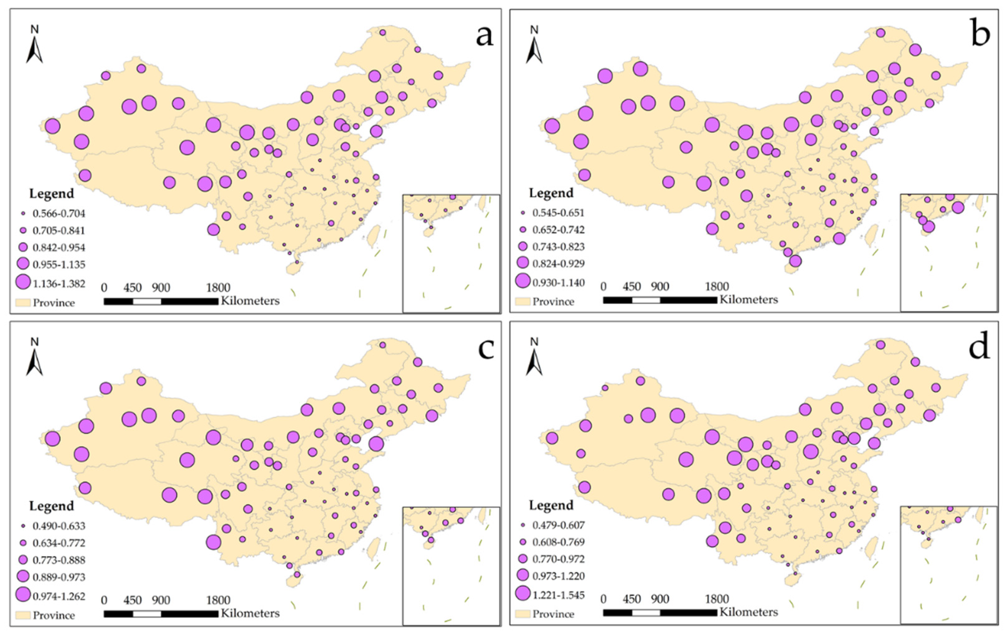
The empirical coefficients of the four models (A-P, Lqbal, Bahel and Sen Models) were calculated using the data from 72 stations with a continuous sunshine duration and solar radiation in China. The error of the four models was checked, and the checking results were determined using , MAE and . Figure 5 shows the error-checking results of the A-P, Lqbal, Bahel and Sen Models for the four seasons. The results show that the nonlinear model proposed by Sen performs well from season to season, with a small MAE (spring: 0.557, summer: 0.615, autumn: 0.405, winter: 0.325), a small (spring: 0.730, summer: 0.799, autumn: 0.539, winter: 0.430) and a large value (spring: 0.837, summer: 0.815, autumn: 0.862, winter: 0.821). There is little difference between the Bahel and Sen Models. However, the A-P linear model and Lqbal quadratic polynomial model perform poorly.

Figure 5.
Error-checking results (MAE (a), RMSE (b) and (c)) for the four models in different seasons.
As the error-checking results of the Bahel and Sen Models are basically the same, we compare the coefficient stability of the two models, as shown in Figure 6. Figure 6a shows the seasonal and annual standard deviation results of the four coefficients of the Bahel Model. Coefficient a (spring: 0.055, summer: 0.039, autumn: 0.045, winter: 0.080, annual: 0.059) changes least among the different stations, and coefficient c (spring: 0.984, summer: 0.995, autumn: 1.098, winter: 1.052, annual: 1.035) changes most. The standard deviations of the four coefficients vary little with respect to the season. Coefficient c, with a large standard deviation, reaches its maximum in autumn and its minimum in spring. In contrast, the three coefficients of the Sen Model have better stability in all seasons (Figure 6b). The standard deviations of empirical coefficient a (spring: 0.051, summer: 0.036, autumn: 0.040, winter: 0.075, annual: 0.055) and b (spring: 0.037, summer: 0.039, autumn: 0.037, winter: 0.061, annual: 0.051) are very small, and that of empirical coefficient c (spring: 0.240, summer: 0.154, autumn: 0.201, winter: 0.299, annual: 0.232) is relatively large. The standard deviations of the three coefficients all reach their maximum values in winter. Empirical coefficient c, which has the greatest influence on the estimation result of the model, reaches its minimum value in summer. In the actual investigation of the empirical coefficients for each station, we found that the values of experience coefficients c (minimum: −7.947, maximum: 0.915) and d (minimum: −0.529, maximum: 5.794) of the Bahel Model had a broad distribution. The value of empirical coefficient c (minimum: −0.086, maximum: 1.545) of the Sen Model had a small distribution. The Sen Model is the most suitable model for solar radiation estimation based on sunshine duration in China compared with the other three models in terms of error and coefficient stability. Therefore, the Sen Model is selected as the best model for the estimation of solar radiation based on sunshine duration in this study. The performance of each model is different from season to season. The MAE and of each model are best in winter and worst in summer; while the performance of in spring and autumn is better than that in summer and winter.

Figure 6.
Degree of dispersion of empirical coefficients for the Bahel Model (a) and Sen Model (b).
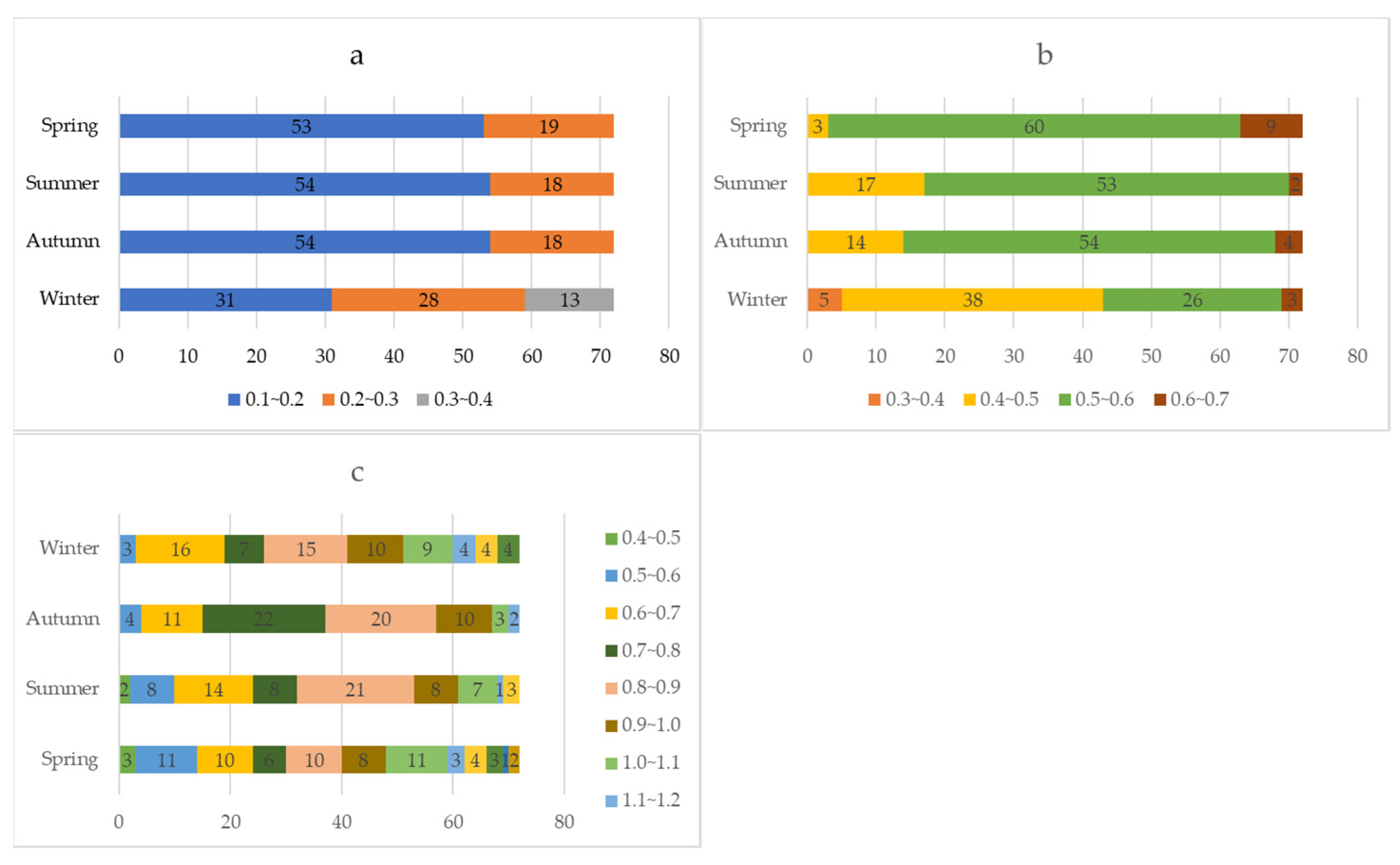
After selecting the Sen Model as the best model, the value changes (Figure 7) and geographical changes (Figure 8) of the empirical coefficients of the Sen Model for the 72 stations are displayed. Figure 7 shows the coefficient distributions for the 72 stations from season to season. Different color blocks represent different value ranges, and the numbers on the color blocks represent the number of meteorological stations within that value range. Coefficient a of the 72 stations lies mainly between 0.1 and 0.2 for the four seasons. In spring, summer and autumn, the coefficients are concentrated, with a distribution range of 0.1–0.3, while in winter, they are relatively dispersed, with a distribution range of 0.1–0.4. The distribution range of coefficient b in spring, summer and autumn is 0.4–0.7, mostly concentrated between 0.5 and 0.6, while in winter, the distribution range is 0.3–0.7, mostly concentrated between 0.4 and 0.6. The distribution of coefficient c is relatively discrete in the four seasons; but the dispersion is high in winter, with a range of 0.4–1.6.

Figure 7.
Distributions of the coefficient a (a), coefficient b (b) and coefficient c (c) for the 72 stations in the Sen Model in different seasons.
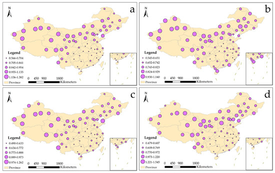
Figure 8.
Geographical changes in coefficient c for the 72 stations in the Sen Model in spring (a), summer (b), autumn (c) and winter (d).
Coefficient c of the Sen Model varies significantly among the different regions and is the coefficient that has the greatest impact on the final distribution results of the PV energy. Therefore, we studied the regional differences of coefficient c. Figure 8 shows the differences in coefficient c for the 72 stations in different regions in spring (Figure 8a), summer (Figure 8b), autumn (Figure 8c) and winter (Figure 8d). Coefficient c varies regularly among the different regions. On the whole, coefficient c is larger in the north, northeast, northwest, west and southwest of China, and smaller in the east, southeast and south. The larger coefficient c is, the more the solar radiation depends on the sunshine percentage; in contrast, other local conditions, except for sunshine percentage, have a significant weakening effect on the solar radiation. This may be because of local environmental conditions. For example, due to the influence of monsoons in southern China, water vapor is abundant throughout the year, which weakens solar radiation through absorption and scattering. Figure 9 shows the average values of the Sen Model coefficients for all stations in the four seasons. The three empirical coefficients of the Sen Model change little in the four seasons, which further illustrates the stability of the Sen Model coefficients.
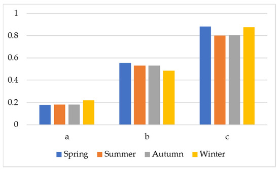
Figure 9.
Seasonal average values of coefficients a, b and c for the Sen Model for all stations.
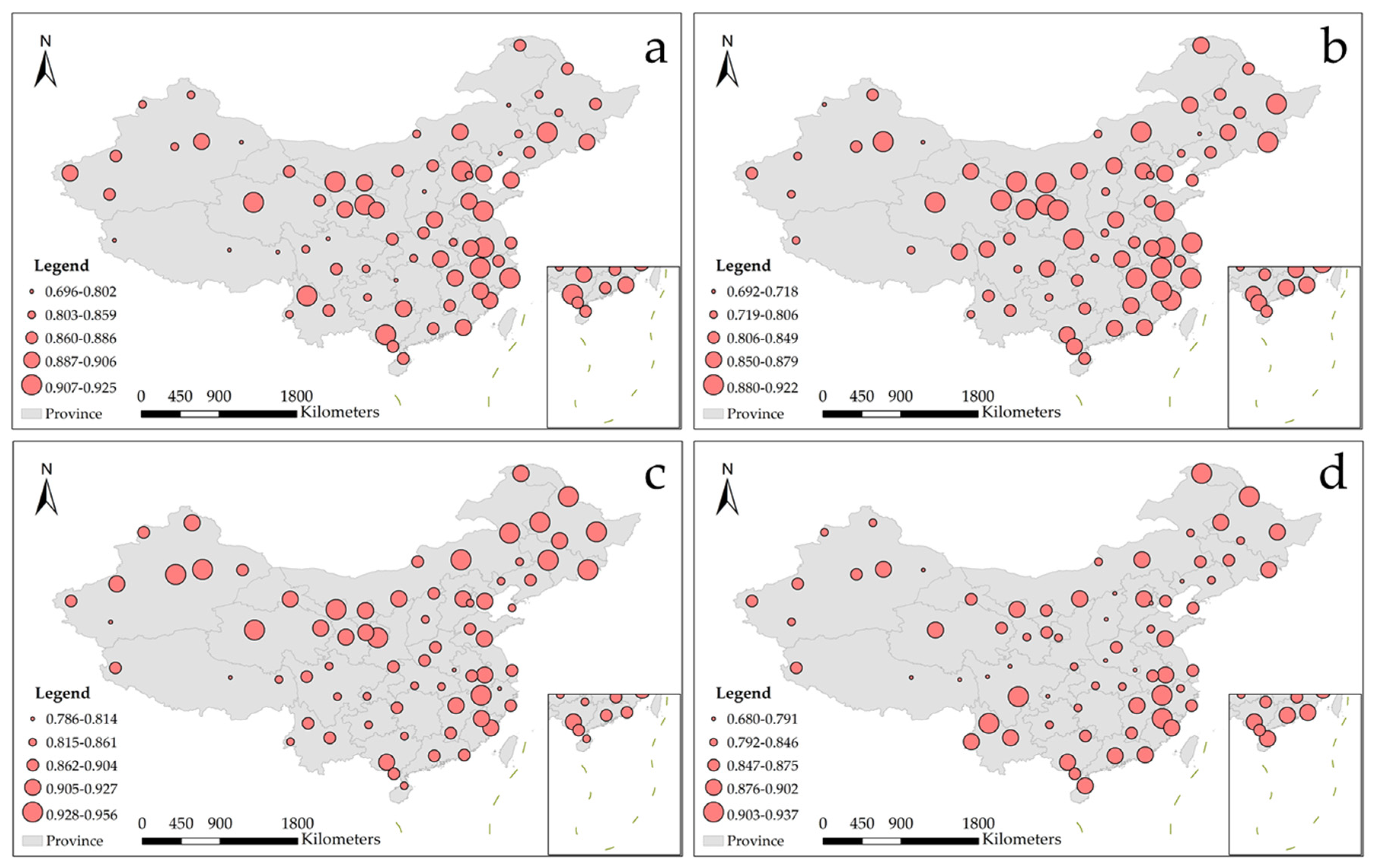
Figure 10 and Figure 11 show the change in the value range and geographical area of the error-checking results for the Sen Model at the 72 stations. Figure 10 shows the distribution of the value range for the 72 stations; points of different colors represent different stations. There are great differences in the error values among the different stations. In spring, the minimum value of MAE is 0.345, and the maximum is 0.710; in summer, the minimum value is 0.390, and the maximum value is 0.807; in autumn, the minimum value is 0.220, and the maximum value is 0.566; and in winter, the minimum value is 0.127, and the maximum value is 0.513. In spring, the minimum value of RMSE is 0.454, and the maximum value is 0.977; in summer, the minimum value is 0.520, and the maximum value is 0.999; in autumn, the minimum value is 0.287, and the maximum value is 0.765; and in winter, the minimum value is 0.173, and the maximum value is 0.679. In spring, the minimum value of is 0.696, and the maximum value is 0.925; in summer, the minimum value is 0.692, and the maximum value is 0.922; in autumn, the minimum value is 0.786, and the maximum value is 0.956; and in winter, the minimum value is 0.680, and the maximum value is 0.937. The errors of the Sen Model vary greatly from season to season. MAE and RMSE are best in winter and worst in summer; and is best in spring and autumn. Figure 11 shows the regional variation in for the 72 stations, for which there is no obvious rule from region to region.

Figure 10.
Numerical range distribution of MAE (a), RMSE (b) and (c) using the Sen Model for the 72 stations.
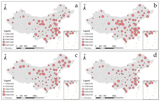
Figure 11.
Regional distribution of for the 72 stations using the Sen Model in spring (a), summer (b), autumn (c) and winter (d).
4.3. Terrain Shielding
After estimating the initial PV energy distribution using the sunshine percentage generated by cloud cover and the Sen Model, the terrain shielding factor was added to the results. In fact, there are not many areas affected by terrain shielding in China, which is commonly seen in mountainous areas with large elevation variations in southwestern China and the mountains in Xinjiang at high latitude. The relatively flat terrain and very low-latitude areas are not often shielded by terrain. Terrain shielding generally occurs in winter but is rare in the other seasons. We take the Altai Mountains in northwest China as an example (Figure 12) to show the distribution of PV energy in early January after adding the terrain shielding factor. Figure 12a is the DEM north of Tianshan Mountain. Figure 12b shows the distribution of PV energy before adding the terrain shielding factor, and Figure 12c shows the distribution of PV energy after adding the terrain shielding factor. Compared with Figure 12b, Figure 12c shows many dark green patches on the shady slope of the mountain, indicating areas with low PV energy. Due to the high latitude of the Altai Mountains and the low solar altitude angle in winter, there is a large area on the shady slope that does not receive sunlight during the day. The experiment proves that terrain factors should be considered during deciding the location of PV power stations.

Figure 12.
Change in the distribution of PV energy before (b) and after (c) adding the terrain shielding factor. (a) is the DEM in the north of Tianshan Mountain.
4.4. PV Energy Distribution
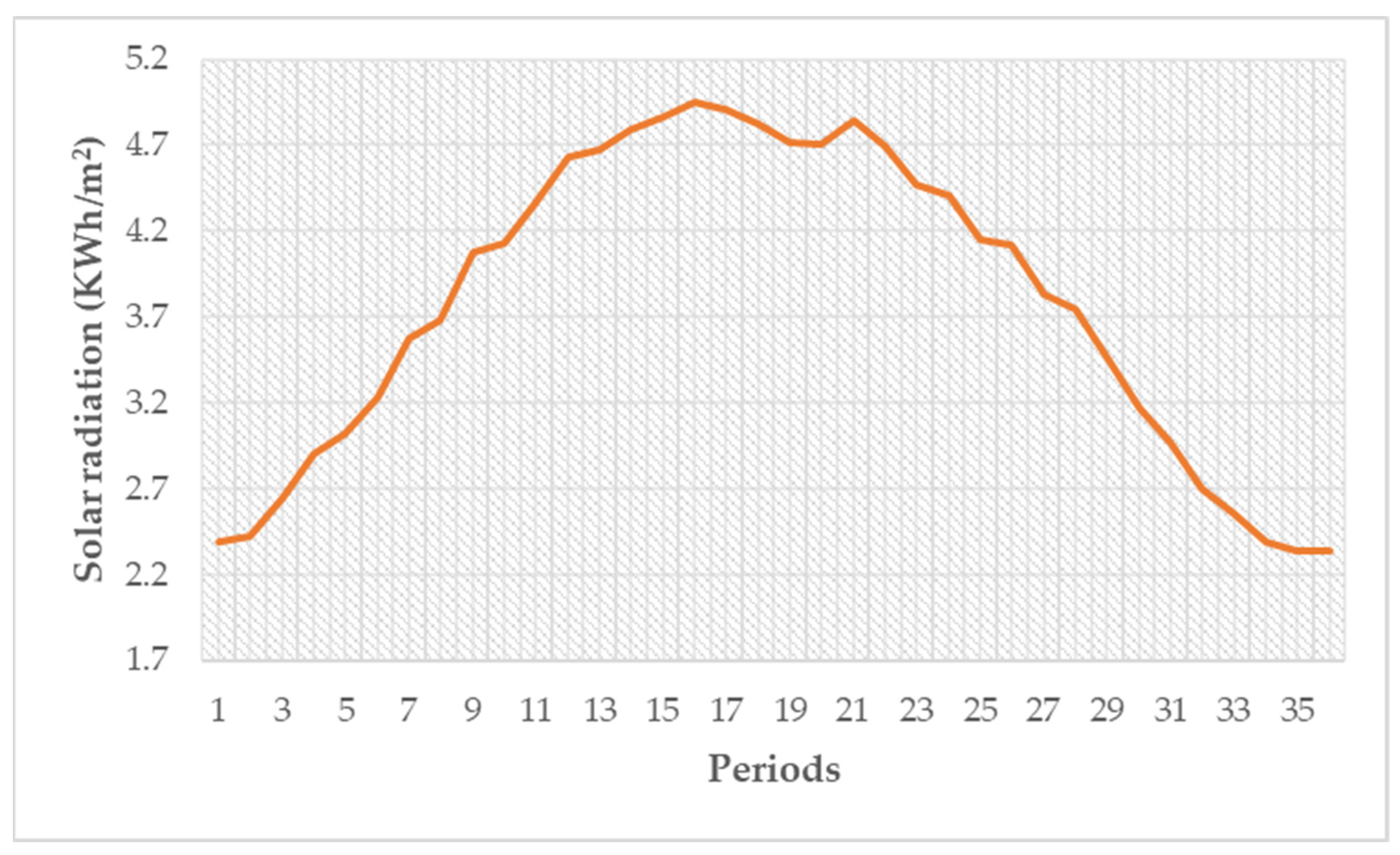
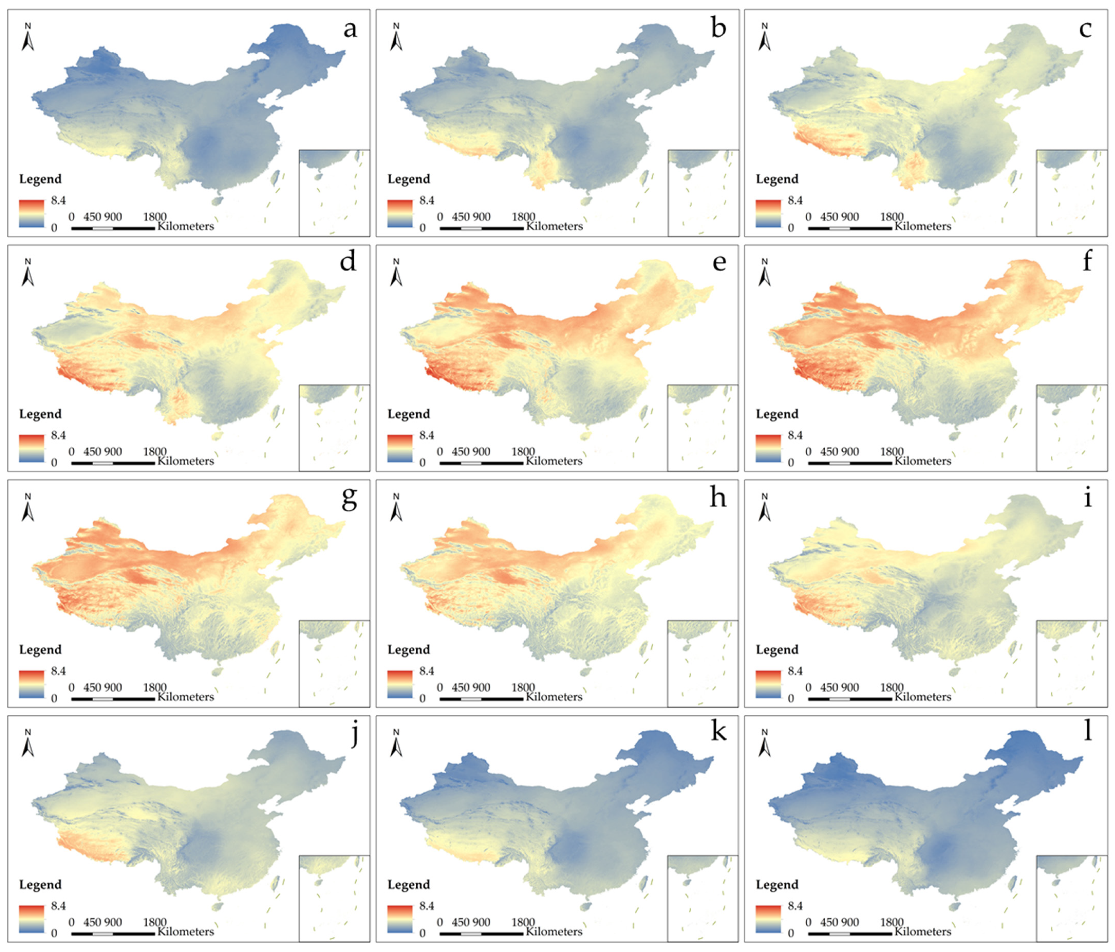
The sunshine percentage data based on cloud cover and the optimal empirical coefficients were substituted into the Sen Model to estimate the PV energy distribution in China combined with terrain shielding. After the estimation of the PV energy distribution, the 10-day average daily total solar radiation in China is finally generated. Figure 13 shows a broken line diagram of the average daily total solar radiation for every 10 days in China, and Figure 14 shows a diagram of the monthly average daily total solar radiation. Figure 13 and Figure 14 show that the daily total PV energy in China increases or decreases regularly according to season. The PV energy in April, May, June, July, August and September are more abundant, located predominantly in the north, northwest, west and southwest of China, but are scarcer in the east, southeast and south. The PV energy in January, February, March, October, November and December are relatively scarce and mainly concentrated in the high-altitude areas in southwestern China.
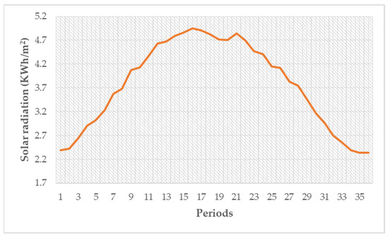
Figure 13.
Change in 10-day average daily total PV energy in China for 36 periods.
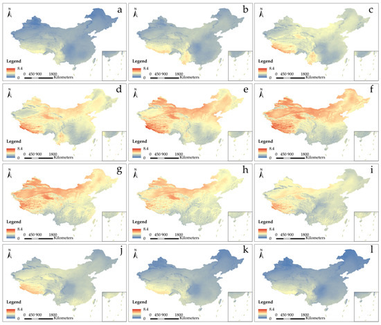
Figure 14.
Monthly average daily total PV energy in China. Images (a–l) show the monthly average daily total solar radiation from January to December.
In order to prove that the GLHCC cloud product produces a more accurate result for the estimation of PV energy, the GHI of the World Bank and the yearly average irradiance of PVGIS are selected for consistency checking. Figure 15a shows the annual average daily total PV energy, with a resolution of 1 km, in this study; Figure 15b shows the GHI data of the World Bank, with a resolution of 250 m; and Figure 15c shows the yearly average global irradiance of PVGIS, with a resolution of 5 km. Since the solar radiation data of PVGIS only include the areas of Africa, part of Europe, part of Asia, part of South America and part of Australia, the solar radiation data does not cover all of China. In addition, the three products are normalized due to their different ways (daily total solar radiation or instantaneous irradiance) of representing the distribution results of PV energy. The PV energy distribution of the three products is roughly the same: The PV energy of the southwest Qinghai-Tibet Plateau and Qaidam Basin is the most abundant, and the PV energy of the Sichuan Basin is the scarcest. The main reason for the regional difference in the distribution of PV energy is that the Qinghai-Tibet Plateau has a high altitude, relatively thin air, little water-vapor content and little cloud cover, all of which only slightly weakens the solar radiation. In addition, due to the low latitude of the Qinghai-Tibet Plateau, the average solar height is larger all year round, and the solar radiation is stronger. The Qaidam Basin is located in the desertification area of northwestern China and is an arid and semi-arid area with little precipitation and long sunshine duration. It is located at high-altitude and, therefore, experiences only limited weakening of solar radiation by the atmosphere. The amount of precipitation in the Sichuan Basin is significant, and water vapor is not easily dispersed, leading to a relatively high number of cloudy days and foggy days. This results in a short sunshine duration, low sunshine intensity and poor solar energy resources.
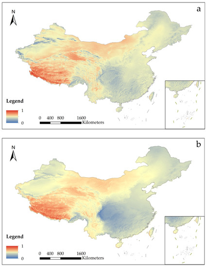
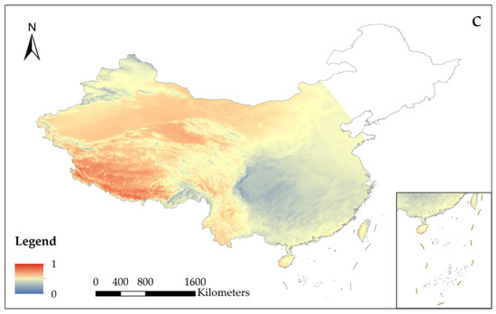
Figure 15.
Comparison of the annual distribution of PV energy (after normalization) in China. (a) Annual average daily total solar radiation data. (b) GHI of the World Bank. (c) Yearly average irradiance from PVGIS.
However, there are still many differences between the three products. Compared with the other two products, the PV energy in this paper is distributed in mountainous areas with more cloud, have lower levels of solar radiation. The main anomaly in the GHI data is that the irradiance of different regions in China has distinct boundaries. For example, the irradiance of the GHI in Xinjiang is significantly smaller than the surrounding irradiance. The other two products have no sudden change in solar radiation, except for the change occurring in the mountains. This may be related to the different model parameters adopted for the different regions in China in the GHI. The irradiance data of PVGIS show lower levels of solar radiation in the area north of Tianshan Mountain than in the surrounding areas, which does not show in the other two products.
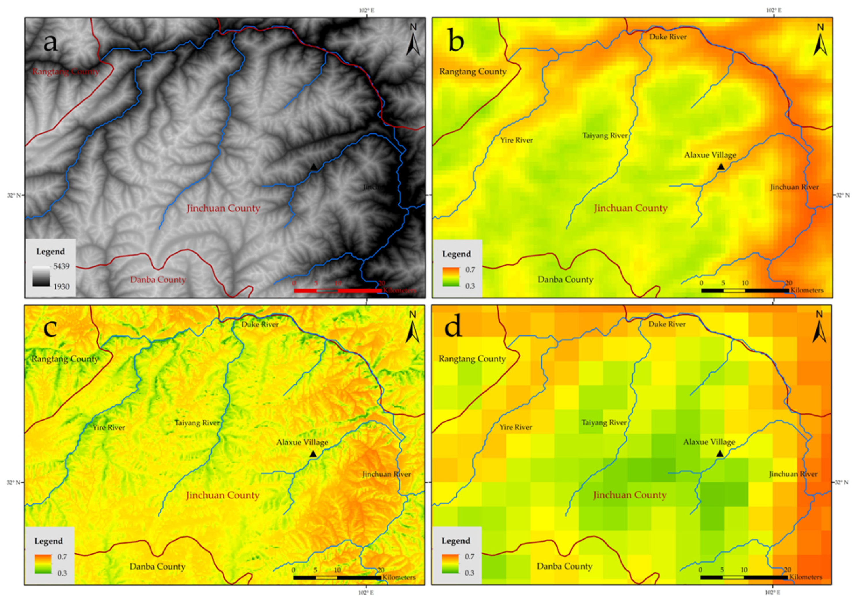
In addition to the above macro differences between the three products, some local details of GHI are different from the distribution of PV energy in this study and the irradiance of PVGIS, mainly in the valley in southwestern China. Jinchuan County in Sichuan province has unique climatic conditions and long sunshine hours. With an annual average sunshine duration of more than 2400 h, it has the reputation of a “plateau sunny city” and is a typical valley county. Therefore, taking Jinchuan County as an example, we show the difference in the PV-resource distribution results of the three products in Figure 16. Figure 16a is the DEM with a resolution of 90 m in Jinchuan County, Figure 16b is the PV energy distribution map of this study (after normalization), Figure 16c is the GHI of the World Bank (after normalization) and Figure 16d shows the irradiance of PVGIS (after normalization). Figure 16 shows that the GHI of the World Bank is more detailed than the PV energy of this study and the irradiance of PVGIS due to the difference in resolution. However, the geographical distribution of PV energy in this study is similar to that of the irradiance of the PVGIS. There is abundant PV energy in the valley area and scarce PV energy on the hillside. However, the geographical distribution of the GHI in this area is opposite to that of the PV energy in this study and the irradiance of the PVGIS. There is a positive correlation between GHI and altitude. The lower the altitude, the lower the solar radiation levels; and the higher the altitude, the higher the solar radiation levels. The distribution of PV energy in this study and PVGIS is more consistent with the fact. Because the valley in this area is a typical dry-hot valley [72]; characterized by dry, hot and plenty of sunshine. Part of the 30 MW PV poverty alleviation project in Jinchuan County, Sichuan province, is built in the sunny Alaxue Village, shown in Figure 16. Although the GHI of the World Bank reaches a spatial resolution of 250 km, it does not reflect the actual PV energy well. Although the current solar radiation products mostly consider the influence of the amount of cloud, cloud amount data are often of low spatial resolution or low precision. The use of the GLHCC cloud amount data in this study greatly improves the spatial resolution and accuracy of the solar radiation products.
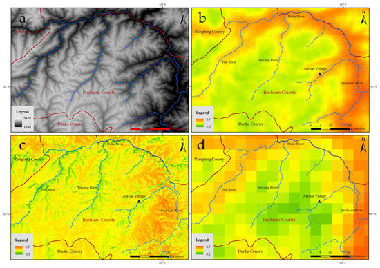
Figure 16.
Distribution of PV energy (after normalization) in Jinchuan County, Sichuan Province. (a) DEM data. (b) Annual average daily total solar-radiation data. (c) GHI of the World Bank. (d) Yearly average irradiance from PVGIS.
It is necessary to explain the causes of dry-hot valleys. Dry-hot valley regions are rich in solar and heat resources, with a hot climate and little rain, which is not as wettish as general valleys [73]. The main influencing factors in the formation of dry-hot valleys are the foehn effect and the local circulation effect of valley winds. The foehn effect arises when foehn winds pass through an area, making the climate hot and dry. Foehn winds are caused by air currents descending over mountains, and their temperature rises by about 10 degrees Celsius for every 1000 m they fall. Valley winds are local winds with a daily cycle, appearing in mountainous areas and surrounding areas. During the day, the hillside receives more heat from the sun, and the air warms more. Over valleys at the same height as mountain tops, the air warms less because it is farther from the ground. Due to the continuous expansion and rise of warm air on the hillside, a low-pressure region is formed near the ground at the top of the mountain and accumulates from the hillside to the valley. The air accumulates from the mountainside over the valley, and the air over the valley contracts and sinks under the influence of gravity. High pressure is formed on the valley ground, and the downdraft forms a dry and hot environment. This local circulation effect of valley winds causes cloud belts to appear on hillsides. Therefore, in a dry-hot valley area, the amount of PV energy should be greater than on a hillside.
5. Discussion
In this study, a 10-day average daily total solar-radiation product with a resolution of 1 km was produced using GLHCC cloud coverage data. It should be noted that the annual average product generated by the 10-day product is only a reference for the selection of PV power stations. The actual terrain conditions, land utilization situations and disaster situations should also be considered in the real process of the station location. We proved the applicability of our product by comparing it with the GHI of the World Bank and the irradiance from PVGIS. Further explanation is needed for a comparison of the results.
Section 4.4 shows that the macro distributions of PV energy for the three products are roughly the same but with some differences. In the comparison for Jinchuan County, the spatial resolution of GHI has an absolute advantage over the PV energy product in this study and the irradiance product of PVGIS. However, the GHI data do not accurately represent the normal solar radiation in a dry-hot valley. This is because the high resolution of the GHI data is derived from the SRTM DEM data rather than from satellite data used to calculate the cloud index or other data sources. The algorithm used in the solar radiation datasets of the World Bank is the Solargis internal algorithm (https://solargis.com/docs/methodology/solar-radiation-modeling (accessed on 13 December 2021)). In this algorithm, the data sources used to calculate the cloud index are Meteosat (Meteorological Satellite), GEOS (Geosynchronous Earth Orbit Satellite), MTSAT (Multi-Function Transport Satellite) and Himawari satellite data sources, with spatial resolutions of 3–4 km. These cloud data, with low resolution, cannot ascertain the cloud cover distribution in a dry-hot valley area. Therefore, although the GHI data have a high resolution and can reflect more topographic details, the distribution of PV energy is not accurate in areas with high spatial variability clouds.
The three products perform differently in different regions, and it is difficult to determine which product is the most accurate overall. However, the products in this study accurately represent PV energy in areas with high spatial variability clouds, such as dry-hot valleys. Dry-hot valleys are not uncommon in China and are mainly distributed in Panzhihua City, Yunnan and Guizhou Provinces along the Jinsha, Yuanjiang, Nujiang and Nanpan Rivers. These regions are important output regions of PV power. Therefore, accurate PV energy distribution data are of great significance for planning PV power stations in these regions. Our experiment proves that if the GLHCC cloud product is applied to a model for other solar radiation products, the product accuracy is improved.
6. Conclusions
In this study, we produced 10-day, monthly, quarterly and yearly PV energy products in China based on GLHCC cloud data, with a resolution of 1 km. Using the GLHCC data in China, this paper created sunshine percentage data using a linear model. The sunshine duration data and solar radiation data of 72 meteorological stations in China were used for quarterly LSF to find the best fitting coefficients for four models. The Sen Model was selected as the most suitable for estimating the PV energy in China through error-checking. Using the sunshine percentage and Sen Model, combined with terrain shielding, a reasonable estimation of the distribution of PV energy was obtained.
The cloud coverage product GLHCC used in this study, which has a higher resolution and higher precision than other cloud products, produced high resolution and precision PV energy distribution data. The consistency checking on three PV products showed that, compared with the irradiance data from PVGIS, the PV data in this paper had a higher spatial resolution, showing more local details. Compared to GHI data, with a resolution of 250 m, the data from our product more accurately represented the distribution of PV energy in areas with high spatial-variability clouds. The annual distribution of PV energy in China obtained in this study reflects the annual power generation potential of China, providing an important reference for the location of PV power stations. The 10-day, monthly and quarterly PV energy distribution products for China can be used to effectively evaluate the PV energy during different periods of the year. The products provide a reference for existing power stations to carry out peak regulation and energy storage and to supplement wind power generation or hydroelectric power generation at appropriate times.
However, there are some deficiencies in this study. First, a relatively simple linear model was adopted to generate sunshine percentage data based on cloud frequency data, using the relationship between cloud cover and sunshine percentage in an ideal state. Therefore, there is a certain error under real environmental and observational conditions. Secondly, the size of a window used in calculating the terrain shielding factor is 3 × 3, the distance range of which is small. Distant mountains that can shield an area are not included in the range of calculation. In future studies, more accurate models will be needed to determine the relationship between cloud cover and sunshine percentage and to calculate multi-scale terrain shielding factors according to different distances.
Author Contributions
Data curation, A.L.; Investigation, S.Z.; Methodology, S.Z. and F.C.; Project administration, Y.M., F.C. and J.L.; Validation, S.Z., E.S. and W.Y.; Writing—original draft, S.Z.; Writing—review and editing, S.Z. and Y.M. All authors have read and agreed to the published version of the manuscript.
Funding
This research was funded by the Key Research and Development Program of Hainan Province (ZDYF2021SHFZ260).
Acknowledgments
Special acknowledgements should be expressed to the Key Laboratory of Earth Observation of Hainan Province, Hainan Research Institute, Aerospace Information Research Institute, Chinese Academy of Sciences.
Conflicts of Interest
The authors declare no conflict of interest.
Abbreviations
| ANN | Artificial Neural Network |
| ASR | Astronomical Solar Radiation |
| CloudSat | Cloud Detecting Satellite |
| DEM | Digital Terrain Elevation Model |
| DIF | Diffuse Horizontal Radiation |
| DNI | Direct Normal Exposure |
| ELM | Extreme Learning Machine |
| EOS | Earth Observing System |
| GEOS | Geosynchronous Earth Orbit Satellite |
| GHI | Global Horizontal Irradiance |
| GLHCC | Global Land High-resolution Cloud Climatology |
| GPR | Gaussian Process Regression |
| GTI | Global Radiation for Optimal Tilted Surfaces |
| IDW | Inverse Distance Weighting |
| ISCCP | International Satellite Cloud Climatology Project |
| LSF | Least Squares Fit |
| MAE | Mean Absolute Error |
| Meteosat | Meteorological Satellite |
| MM | Markov Model |
| MODIS | Moderate-Resolution Imaging Spectroradiometer |
| MTSAT | Multi-Function Transport Satellite |
| NASA | National Aeronautics and Space Administration |
| NOAA | National Oceanic and Atmospheric Administration |
| NSRDB | National Solar Radiation Database |
| OPTA | Optimal Tilt of Photovoltaic Modules |
| PATMOS-X | Pathfinder Atmospheres—Extended |
| PV | Photovoltaic |
| PVGIS | Photovoltaic Geographic Information System |
| PVOUT | Photovoltaic Power Potential |
| RF | Random Forest |
| RMSE | Root Mean Square Error |
| SRTM | Shuttle Radar Topography Mission |
| SVM | Support Vector Machine |
| TEMP | Air Temperature 2 m above ground |
References
- Pandey, A.K.; Tyagi, V.V.; Selvaraj, J.A.L.; Rahim, N.A.; Tyagi, S.K. Recent advances in solar photovoltaic systems for emerging trends and advanced applications. Renew. Sustain. Energy Rev. 2016, 53, 859–884. [Google Scholar] [CrossRef]
- Niu, D.X.; Zhen, H.; Yu, M.; Wang, K.K.; Sun, L.J.; Xu, X.M. Prioritization of renewable energy alternatives for China by using a hybrid FMCDM methodology with uncertain information. Sustainability 2020, 12, 4649. [Google Scholar] [CrossRef]
- Fu, J.; Xu, J.; Liu, Y.; Xie, L.; Liu, S. China actively promotes CO2 capture, utilization and storage research to achieve carbon peak and carbon neutrality. Adv. Geo-Energy Res. 2022, 6, 1–3. [Google Scholar]
- Barragan-Escandon, A.; Zalamea-Leon, E.; Terrados-Cepeda, J. Incidence of photovoltaics in cities based on indicators of occupancy and urban sustainability. Energies 2019, 12, 810. [Google Scholar] [CrossRef] [Green Version]
- Olowu, T.O.; Sundararajan, A.; Moghaddami, M.; Sarwat, A.I. Future challenges and mitigation methods for high photovoltaic penetration: A survey. Energies 2018, 11, 1782. [Google Scholar] [CrossRef] [Green Version]
- Gairaa, K.; Khellaf, A.; Messlem, Y.; Chellali, F. Estimation of the daily global solar radiation based on Box-Jenkins and ANN models: A combined approach. Renew. Sustain. Energy Rev. 2016, 57, 238–249. [Google Scholar] [CrossRef]
- Dumas, A.; Andrisani, A.; Bonnici, M.; Graditi, G.; Leanza, G.; Madonia, M.; Trancossi, M. A new correlation between global solar energy radiation and daily temperature variations. Sol. Energy 2015, 116, 117–124. [Google Scholar] [CrossRef]
- Doljak, D.; Stanojevic, G. Evaluation of natural conditions for site selection of ground-mounted photovoltaic power plants in Serbia. Energy 2017, 127, 291–300. [Google Scholar] [CrossRef] [Green Version]
- Agyekum, E.B.; Amjad, F.; Shah, L.; Velkin, V.I. Optimizing photovoltaic power plant site selection using analytical hierarchy process and density-based clustering—Policy implications for transmission network expansion, Ghana. Sustain. Energy Technol. 2021, 47, 101521. [Google Scholar] [CrossRef]
- Liu, X.Y.; Mei, X.R.; Li, Y.Z.; Zhang, Y.Q.; Wang, Q.S.; Jensen, F.R.; Porter, J.R. Calibration of the Angstrom-Prescott coefficients (a, b) under different time scales and their impacts in estimating global solar radiation in the Yellow River basin. Agric. For. Meteorol. 2009, 149, 697–710. [Google Scholar] [CrossRef]
- Tang, W.J.; Yang, K.; Qin, J.; Min, M. Development of a 50-year daily surface solar radiation dataset over China. Sci. China Earth Sci. 2013, 56, 1555–1565. [Google Scholar] [CrossRef]
- Li, M.F.; Fan, L.; Liu, H.B.; Guo, P.T.; Wu, W. A general model for estimation of daily global solar radiation using air temperatures and site geographic parameters in Southwest China. J. Atmos. Sol.-Terr. Phy. 2013, 92, 145–150. [Google Scholar] [CrossRef]
- Kimball, H.H. Variations in the total and luminous solar radiation with geographical position in the United State, Mn. Weather Rev. 1919, 47, 769–793. [Google Scholar] [CrossRef]
- Angstrom, A. Solar and atmospheric radiation. Q. J. Roy. Meteor. Soc. 1924, 20, 121–126. [Google Scholar] [CrossRef]
- Zhang, J.Y.; Zhao, L.; Deng, S.; Xu, W.C.; Zhang, Y. A critical review of the models used to estimate solar radiation. Renew. Sustain. Energy Rev. 2017, 70, 314–329. [Google Scholar] [CrossRef]
- Qin, W.M.; Wang, L.C.; Lin, A.W.; Zhang, M.; Xia, X.G.; Hu, B.; Niu, Z.G. Comparison of deterministic and data-driven models for solar radiation estimation in China. Renew. Sustain. Energy Rev. 2018, 81, 579–594. [Google Scholar] [CrossRef]
- Fan, J.L.; Wu, L.F.; Zhang, F.C.; Cai, H.J.; Ma, X.; Bai, H. Evaluation and development of empirical models for estimating daily and monthly mean daily diffuse horizontal solar radiation for different climatic regions of China. Renew. Sustain. Energy Rev. 2019, 105, 168–186. [Google Scholar] [CrossRef]
- Agbulut, U.; Gurel, A.E.; Bicen, Y. Prediction of daily global solar radiation using different machine learning algorithms: Evaluation and comparison. Renew. Sustain. Energy Rev. 2021, 135, 110114. [Google Scholar] [CrossRef]
- Stanciu, C.; Stanciu, D. Optimum tilt angle for flat plate collectors all over the World—A declination dependence formula and comparisons of three solar radiation models. Energy Convers. Manag. 2014, 81, 133–143. [Google Scholar] [CrossRef]
- Hottel, M.C.; Woertz, B.B. Performance of flat plate solar heat collectors. Trans. ASME 1942, 64, 91–104. [Google Scholar]
- Liu, B.Y.H.; Jordan, R.C. The Interrelationship and Characteristic Distribution of Direct, Diffuse and Total Solar Radiation. Sol. Energy 1960, 4, 1–19. [Google Scholar] [CrossRef]
- Cai, T.; Duan, S.X.; Chen, C.S. Forecasting power output for grid-connected photovoltaic power system without using solar radiation measurement. In Proceedings of the 2nd International Symposium on Power Electronics for Distributed Generation Systems, Hefei, China, 16–18 June 2010; pp. 773–777. [Google Scholar]
- Abouhashish, M. Applicability of ASHRAE clear-sky model based on solar-radiation measurements in Saudi Arabia. AIP Conf. Proc. 2017, 1850, 140001. [Google Scholar]
- Olatomiwa, L.; Mekhilef, S.; Shamshirband, S.; Petkovic, D. Adaptive neuro-fuzzy approach for solar radiation prediction in Nigeria. Renew. Sustain. Energy Rev. 2015, 51, 1784–1791. [Google Scholar] [CrossRef]
- Amrouche, B.; Le Pivert, X. Artificial neural network based daily local forecasting for global solar radiation. Appl. Energy 2014, 130, 333–341. [Google Scholar] [CrossRef]
- Olatomiwa, L.; Mekhilef, S.; Shamshirband, S.; Mohammadi, K.; Petkovic, D.; Sudheer, C. A support vector machine firefly algorithm-based model for global solar radiation prediction. Sol. Energy 2015, 115, 632–644. [Google Scholar] [CrossRef]
- Jiang, H.; Dong, Y. A nonlinear support vector machine model with hard penalty function based on glowworm swarm optimization for forecasting daily global solar radiation. Energy Convers. Manag. 2016, 126, 991–1002. [Google Scholar] [CrossRef]
- Aguiar, R.J.; Collarespereira, M.; Conde, J.P. Simple procedure for generating sequences of daily radiation values using a library of Markov transition matrices. Sol. Energy 1988, 40, 269–279. [Google Scholar] [CrossRef]
- Bhardwaj, S.; Sharma, V.; Srivastava, S.; Sastry, O.S.; Bandyopadhyay, B.; Chandel, S.S.; Gupta, J.R.P. Estimation of solar radiation using a combination of Hidden Markov Model and generalized Fuzzy model. Sol. Energy 2013, 93, 43–54. [Google Scholar] [CrossRef]
- Sahin, M.; Kaya, Y.; Uyar, M.; Yildirim, S. Application of extreme learning machine for estimating solar radiation from satellite data. Int. J. Energy Res. 2014, 38, 205–212. [Google Scholar] [CrossRef]
- Shamshirband, S.; Mohammadi, K.; Yee, P.L.; Petkovic, D.; Mostafaeipour, A. A comparative evaluation for identifying the suitability of extreme learning machine to predict horizontal global solar radiation. Renew. Sustain. Energy Rev. 2015, 52, 1031–1042. [Google Scholar] [CrossRef]
- Benali, L.; Notton, G.; Fouilloy, A.; Voyant, C.; Dizene, R. Solar radiation forecasting using artificial neural network and random forest methods: Application to normal beam, horizontal diffuse and global components. Renew. Energy 2019, 132, 871–884. [Google Scholar] [CrossRef]
- Babar, B.; Luppino, L.T.; Bostrom, T.; Anfinsen, S.N. Random forest regression for improved mapping of solar irradiance at high latitudes. Sol. Energy 2020, 198, 81–92. [Google Scholar] [CrossRef]
- Guermoui, M.; Gairaa, K.; Rabehi, A.; Djafer, D.; Benkaciali, S. Estimation of the daily global solar radiation based on the Gaussian process regression methodology in the Saharan climate. Eur. Phys. J. Plus 2018, 133, 211. [Google Scholar] [CrossRef]
- Rohani, A.; Taki, M.; Abdollahpour, M. A novel soft computing model (Gaussian process regression with K-fold cross validation) for daily and monthly solar radiation forecasting (Part: I). Renew. Energy 2018, 115, 411–422. [Google Scholar] [CrossRef]
- Prescott, J.A. Evaporation from a water surface in relation to solar radiation. Trans. R. Soc. Aust. 1940, 46, 114–118. [Google Scholar]
- Iqbal, M. Correlation of Average Diffuse and Beam Radiation with Hours of Bright Sunshine. Sol. Energy 1979, 23, 169–173. [Google Scholar] [CrossRef]
- Bahel, V.; Bakhsh, H.; Srinivasan, R. A Correlation for Estimation of Global Solar-Radiation. Energy 1987, 12, 131–135. [Google Scholar] [CrossRef]
- Black, J.N.; Bonython, C.W.; Prescott, J.A. Solar Radiation and the Duration of Sunshine. Q. J. Roy. Meteor. Soc. 1954, 80, 231–235. [Google Scholar] [CrossRef]
- Coppolino, S. A New Correlation between Clearness Index and Relative Sunshine. Renew. Energy 1994, 4, 417–423. [Google Scholar] [CrossRef]
- Almorox, J.; Bocco, M.; Willington, E. Estimation of daily global solar radiation from measured temperatures at Canada de Luque, Cordoba, Argentina. Renew. Energy 2013, 60, 382–387. [Google Scholar] [CrossRef] [Green Version]
- Yacef, R.; Benghanem, M.; Mellit, A. Prediction of daily global solar irradiation data using Bayesian neural network: A comparative study. Renew. Energy 2012, 48, 146–154. [Google Scholar] [CrossRef]
- Nunez, M.; Li, Y. A cloud-based reconstruction of surface solar radiation trends for Australia. Theor. Appl. Climatol. 2008, 91, 59–75. [Google Scholar] [CrossRef]
- Badescu, V.; Dumitrescu, A. Simple solar radiation modelling for different cloud types and climatologies. Theor. Appl. Climatol. 2016, 124, 141–160. [Google Scholar] [CrossRef]
- Almorox, J.; Hontoria, C. Global solar radiation estimation using sunshine duration in Spain. Energy Convers. Manag. 2004, 45, 1529–1535. [Google Scholar] [CrossRef]
- Besharat, F.; Dehghan, A.A.; Faghih, A.R. Empirical models for estimating global solar radiation: A review and case study. Renew. Sustain. Energy Rev. 2013, 21, 798–821. [Google Scholar] [CrossRef]
- Guermoui, M.; Melgani, F.; Gairaa, K.; Mekhalfi, M.L. A comprehensive review of hybrid models for solar radiation forecasting. J. Clean Prod. 2020, 258, 120357. [Google Scholar] [CrossRef]
- Zhou, J.; Wu, Y.Z.; Yan, G. General formula for estimation of monthly average daily global solar radiation in China. Energy Convers. Manag. 2005, 46, 257–268. [Google Scholar]
- Wu, G.F.; Liu, Y.L.; Wang, T.J. Methods and strategy for modeling daily global solar radiation with measured meteorological data—A case study in Nanchang station, China. Energy Convers. Manag. 2007, 48, 2447–2452. [Google Scholar] [CrossRef]
- Li, H.S.; Ma, W.B.; Lian, Y.W.; Wang, X.L.; Zhao, L. Global solar radiation estimation with sunshine duration in Tibet, China. Renew. Energy 2011, 36, 3141–3145. [Google Scholar] [CrossRef]
- Yao, W.X.; Li, Z.R.; Wang, Y.Y.; Jiang, F.J.; Hu, L.Z. Evaluation of global solar radiation models for Shanghai, China. Energy Convers. Manag. 2014, 84, 597–612. [Google Scholar] [CrossRef]
- Rangarajan, S.; Swaminathan, M.S.; Mani, A. Computation of solar-radiation from observations of cloud cover. Sol. Energy 1984, 32, 553–556. [Google Scholar] [CrossRef]
- Sarkar, M.N.I. Estimation of solar radiation from cloud cover data of Bangladesh. Renewables 2016, 3, 11. [Google Scholar] [CrossRef] [Green Version]
- Shi, G.P.; Qiu, X.F.; Zeng, S.; Qiu, Y.P. Remote sensing integration model of sunshine percentage based on cloud cover images. J. Remote Sens. 2013, 7, 1508–1517. [Google Scholar]
- Morf, H. Sunshine and cloud cover prediction based on Markov processes. Sol. Energy 2014, 110, 615–626. [Google Scholar] [CrossRef]
- Zhu, W.W.; Wu, B.F.; Yan, N.N.; Ma, Z.H.; Wang, L.J.; Liu, W.J.; Xing, Q.; Xu, J.M. Estimating Sunshine Duration Using Hourly Total Cloud Amount Data from a Geostationary Meteorological Satellite. Atmosphere 2020, 11, 26. [Google Scholar] [CrossRef] [Green Version]
- Heidinger, A.; Foster, M.; Botambekov, D.; Hiley, M.; Walther, A.; Li, Y. Using the NASA EOS A-Train to probe the performance of the NOAA PATMOS-x cloud fraction CDR. Remote Sens. 2016, 8, 511. [Google Scholar] [CrossRef] [Green Version]
- Foster, M.J.; Heidinger, A. PATMOS-x: Results from a diurnally corrected 30-yr satellite cloud climatology. J. Clim. 2013, 26, 414–425. [Google Scholar] [CrossRef]
- Schiffer, R.A.; Rossow, W.B. The International-Satellite-Cloud-Climatology-Project (Isccp)—The 1st project of the world climate research programme. Bull. Am. Meteorol. Soc. 1983, 64, 779–784. [Google Scholar] [CrossRef] [Green Version]
- Rossow, W.B.; Schiffer, R.A. Isccp cloud data products. Bull. Am. Meteorol. Soc. 1991, 72, 2–20. [Google Scholar] [CrossRef]
- Barnes, W.L.; Pagano, T.S.; Salomonson, V.V. Prelaunch characteristics of the moderate resolution imaging spectroradiometer (MODIS) on EOS-AM1. IEEE Trans. Geosci. Remote Sens. 1998, 36, 1088–1100. [Google Scholar] [CrossRef] [Green Version]
- Vane, D.; Stephens, G.L. The CloudSat mission and the A-Train: A revolutionary approach to observing earth’s atmosphere. In Proceedings of the 2008 IEEE Aerospace Conference, Big Sky, MT, USA, 1–8 March 2008; pp. 1–5. [Google Scholar]
- Zhang, S.Y.; Ma, Y.; Chen, F.; Shang, E.P.; Yao, W.T.; Qiu, Y.B.; Liu, J.B. Global land high-resolution cloud climatology based on an improved MOD09 cloud mask. Remote Sens. 2021, 13, 3997. [Google Scholar] [CrossRef]
- Sengupta, M.; Xie, Y.; Lopez, A.; Habte, A.; Maclaurin, G.; Shelby, J. The National Solar Radiation Data Base (NSRDB). Renew. Sustain. Energy Rev. 2018, 89, 51–60. [Google Scholar] [CrossRef]
- Sen, Z. Simple nonlinear solar irradiation estimation model. Renew. Energy 2007, 32, 342–350. [Google Scholar] [CrossRef]
- Zeng, Y.; Qiu, X.F.; Liu, S.M. Distributed modeling of extraterrestrial solar radiation over rugged terrains. Chin. J. Geophys. 2005, 48, 1028–1033. [Google Scholar]
- Dozier, J.; Frew, J. Rapid calculation of terrain parameters for radiation modeling from digital elevation data. IEEE Trans. Geosci. Remote Sens. 1990, 28, 963–969. [Google Scholar] [CrossRef]
- Bocquet, G. Method of study and cartography of the potential sunny periods in mountainous areas. J. Climatol. 1984, 4, 587–596. [Google Scholar] [CrossRef]
- Li, X.; Cheng, G.D.; Chen, X.Z.; Lu, L. Modification of solar radiation model over rugged terrain. Chin. Sci. Bull. 1999, 44, 1345–1350. [Google Scholar] [CrossRef]
- Zeng, Y.; Qiu, X.F.; Miao, Q.L.; Liu, C.M. Distribution of possible sunshine durations over rugged terrains of China. Prog. Nat. Sci.-Mater. 2003, 13, 761–764. [Google Scholar] [CrossRef]
- Zhu, X.C.; Qiu, X.F.; Zeng, Y.; Gao, J.Q.; He, Y.J. A remote sensing model to estimate sunshine duration in the Ningxia Hui Autonomous Region, China. J. Meteorol. Res. 2015, 29, 144–154. [Google Scholar] [CrossRef]
- Zhang, J.P.; Yang, Z.; Wang, D.J.; Zhang, X.B. Climate change and causes in the Yuanmou dry-hot valley of Yunnan, China. J. Arid Environ. 2002, 51, 153–162. [Google Scholar]
- Wang, D.C.; Wang, F.C.; Huang, Y.; Duan, X.; Liu, J.Y.; Hu, B.X.; Sun, Z.C.; Chen, J.H. Examining the effects of hydropower station construction on the surface temperature of the Jinsha River dry-hot valley at different seasons. Remote Sens. 2018, 10, 600. [Google Scholar] [CrossRef] [Green Version]
Publisher’s Note: MDPI stays neutral with regard to jurisdictional claims in published maps and institutional affiliations. |
© 2022 by the authors. Licensee MDPI, Basel, Switzerland. This article is an open access article distributed under the terms and conditions of the Creative Commons Attribution (CC BY) license (https://creativecommons.org/licenses/by/4.0/).

