Technical Note

Classification of Wetland Vegetation Based on NDVI Time Series from the HLS Dataset

1
Environmental Science Graduate Program, Ohio State University, Columbus, OH 43210, USA
2
Department of Civil, Environmental & Geodetic Engineering, Ohio State University, Columbus, OH 43210, USA
*
Author to whom correspondence should be addressed.
Remote Sens. 2022, 14(9), 2107; https://doi.org/10.3390/rs14092107
Submission received: 31 March 2022 / Revised: 21 April 2022 / Accepted: 25 April 2022 / Published: 27 April 2022
(This article belongs to the Special Issue Advances in Remote Sensing of the Inland and Coastal Water Zones)

Abstract

:
Natural wetlands are intrinsically heterogeneous and typically composed of a mosaic of ecosystem patches with different vegetation types. Hydrological and biogeochemical processes in wetlands vary strongly among these ecosystem patches. To date, most remote sensing classification approaches for wetland vegetation either rely on coarse images that cannot capture the spatial variability of wetland vegetation or rely on very-high-resolution multi-spectral images that are detailed but very sporadic in time (less than once per year). This study aimed to use NDVI time series, generated from NASA’s HLS dataset, to classify vegetation patches. We demonstrate our approach at a temperate, coastal lake, estuarine marsh. To classify vegetation patches, a standard time series library of the four land-cover patch types was built from referencing specific locations that were identified as “pure” pixels. These were identified using a single-time high-resolution image. We calculated the distance between the HLS-NDVI time series at each pixel and the “pure”-pixel standards for each land-cover type. The resulting true-positive classified rate was >73% for all patch types other than water lily. The classification accuracy was higher in pixels of a more uniform composition. A set of vegetation maps was created for the years 2016 to 2020 at our research site to identify the vegetation changes at the site as it is affected by rapid water elevation increases in Lake Erie. Our results reveal how changes in water elevation have changed the patch distribution in significant ways, leading to the local extinction of cattail by 2019 and a continuous increase in the area cover of water lily patches.

1. Introduction

Coastal wetlands provide critical ecosystem services, such as wildlife habitat, fisheries support, carbon sequestration, flood protection, and water quality improvement. Specifically, around the US Great Lakes, as Harmful Algal Bloom (HAB) events are intensifying in extent and frequency, coastal wetlands are becoming increasingly important for mitigating nutrient runoff from agriculturally dominated watersheds to the lakes [1]. Natural wetlands are intrinsically heterogeneous and are typically composed of a mosaic of ecosystem patches with different plant types and hydrological conditions. The adaptation of these plant communities to a water-dominated environment is the basis for their use in improving the water quality in constructed wetlands [2]. Understanding the effects of wetland vegetation on the environmental conditions and ecological function of the wetland is key to determining which plants to grow in a constructed wetland with regards to the specific goals of the wetland-construction project (e.g., maximizing nutrient removal), and to correctly model the global contribution of wetlands to global greenhouse gas emissions and carbon sequestration. Wetland vegetation generates drag on the flow and therefore can influence the water movement through and around a vegetated patch [3]. The plant density and life forms affect the drag and thus control the flow velocity and residence time of the water in different parts of the wetlands, as well as the rate of deposition of suspended solids [4]. Furthermore, emergent plants with high transpiration rates can lower the water level [5]. The rates of nitrogen processing also vary among wetland vegetation communities [6]. Emergent vegetation shows a higher nitrogen retention rate and is more efficient at removing nitrogen than submerged macrophytes [7]. Identifying patch types is particularly important in predicting their contribution to nutrient uptake and sedimentation in coastal wetlands in agricultural watersheds, where the wetlands provide a last “line of defense” to improve runoff water quality. Vegetation uptakes carbon by photosynthesis, and different plants have different characteristic leaf areas and photosynthesis rates. Furthermore, vegetation plays an important role in methane transport, and, thus, the vegetation patch types have a strong impact on carbon sequestration and greenhouse gas flux rates in wetlands [8,9,10,11].
Traditionally, mapping the vegetation communities in a wetland requires intensive fieldwork, and some wetland areas are not easy to access. Remote sensing provides an effective, scalable, and economical alternative by which to monitor and map plant communities in wetlands. Many studies have been conducted to discern wetland vegetation communities using remote sensing imagery. Multispectral remote sensing data, for example, Landsat imagery and hyperspectral remote sensing imagery, have been used to discriminate and map wetland vegetation types [12,13,14,15,16,17]. However, classifying wetland plants comes with additional challenges in comparison to classification of dryland terrestrial plants [18]. Specifically, the boundaries between vegetation patches within a wetland are difficult to identify because of the intrinsically small scale of the wetlands and patches within them, combined with the short ecotones and sharp demarcation between vegetation patches, which is caused by the small scale of the spatial variability of wetland vegetation [17,19,20]. Thus, moderate-resolution remote sensing imagery, for example, MODIS, which has 250 m spatial resolution, is usually not sufficient for differentiating wetland vegetation patches.
The other challenge in classifying wetland vegetation is that the reflectance of different types of wetland canopies is often very similar, and these indistinct reflectance signatures are combined with the reflectance of the underlying soil and water surface [21,22,23]. To overcome this difficulty, high spatial resolution imagery has been used to perform the classification to reduce the spectral mixing effect of different wetland vegetations and underlying soil or hydrological regimes within single pixel [24,25,26]. However, high spatial resolution imagery is typically only available for a given wetland (a small location) with a very sparse return time (at best, 2–3 cloud-free images per year, usually less, and, in most years and locations, none). Therefore, it is not guaranteed that the imagery covers the wetland of interest during the growing season when the vegetation is visible. Alternatively, the spectral difference of wetland vegetation at different times of the year has been demonstrated to be effective in discriminating dryland vegetation types globally [27] and, specifically, in arid/semiarid regions’ dryland vegetation [28]. This approach has been demonstrated in wetlands for the identification of individual target wetland plant species in salt marshes [28,29,30,31]. Similar to our work, Sun et al. [32] used a time series of the Normalized Difference Vegetation Index (NDVI) derived from HJ-1 at a 30 m resolution to classify and map multiple vegetations at a salt marsh in China, but did not continue to monitor vegetation changes over a long (multiple years) period. Sun et al. [32] further indicated the Landsat data are suitable for similar analyses. Not every remote sensing dataset is suitable for constructing time series in terms of wetland vegetation classification. Moderate spatial resolution data have more frequent and regularly repeated images of the same location, which is important for constructing a time series, but its spatial resolution is not high enough to discern the patches of different wetland vegetation types. Moreover, the frequent cloud cover in coastal region results in significant data gaps in remote sensing data [32]. The harmonization of the Landsat and Sentinel-2 (HLS) data by NASA has made it possible to acquire imagery at a moderate-to-high spatial resolution and at a high temporal resolution, which has created the opportunity to build time series of wetland vegetation characteristics at sufficient spatial and temporal resolutions. NDVI is one of the most widely used indices to assess vegetation from remote sensing imagery, and the construction of the NDVI time series has enabled the quantification of the penological dynamics of different wetland vegetations.
The overall goal of this study was to develop a classification approach for wetland vegetation that utilizes vegetation-type characteristic plant phenology, as observed by the NDVI time series from NASA’s HLS dataset. The classification approach that we demonstrate and test here could be used to classify wetland vegetation on a large scale.

2. Materials and Methods
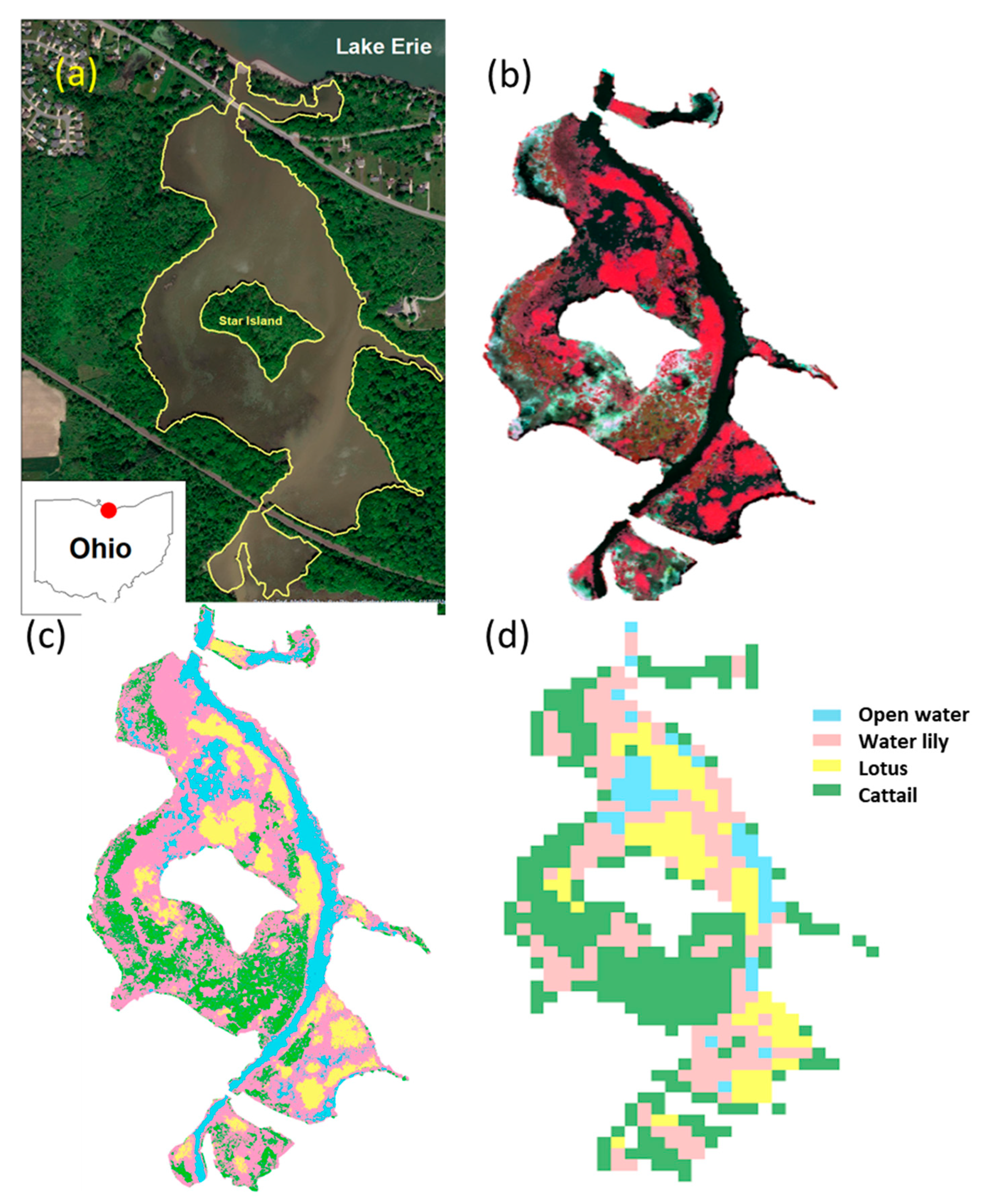
2.1. Study Area

The study was focused on Old Woman Creek (OWC) National Estuarine Research Reserve (NERR) (Figure 1a). It is a temperate, mineral soil, estuarine marsh, located at the south-central shore of Lake Erie, longitude: −82°30′3″, Latitude: 41°22′39″. It is an Ohio State nature preserve and is managed as a cooperative partnership between NOAA NERR and the Ohio Department of Natural Resources (ODNR). It experiences rapid fluctuations in hydrology and water levels as the river mouth is periodically blocked by a sand barrier that is deposited at the lake shore and affected by additional long-term (interannual) water level fluctuations due to the recent water elevation increase of Lake Erie (~1 m over the last decade). OWC was selected for this study because it represents many coastal wetlands of the Great Lakes region. It includes 61 Ha of natural wetland area, currently consisting of four characteristic vegetation patch types. These patch types are defined through their vegetation status, i.e., (1) open water; (2) mud flats; or subclassified among types of patches with emergent vegetation according to the most common (by area) emergent vegetation species. These vegetated types are: (3) American water lily (Nymphaea odorata), (4) yellow lotus (Nelumbo lutea), (5) cattail (several species and hybrids of Typha spp.), and (6) reed (several species of Phragmites spp.). During the past 10 years, patches of reed as well as mud flats have been present, although they occupied a very small (<5%) fraction of the area. However, due to the rising water levels of Lake Erie and the consequent deepening of the wetland water, the mud flats disappeared by 2016, reed in 2018, and cattail in 2020. As our analysis centers on 2017–2020, the only patch types we considered were: open water, water lily, lotus, and cattail. Long-term meteorological, hydrological, and water quality data for OWC are available through the NERR data interface https://cdmo.baruch.sc.edu/ (31 December 2021); long-term radiation, energy, and carbon flux data are available through the Ameriflux database, site ID US-OWC [33].

2.2. Remote Sensing Data

NASA’s Harmonized Landsat and Sentinel-2 (HLS) dataset [34] was used in this study to generate an NDVI time series. This dataset provides consistent surface reflectance from the Landsat 8, Sentinel-2A, and Sentinel-2B satellites. The merged product was run though a set of algorithms that include atmospheric correction, cloud and cloud-shadow masking, spatial co-registration and common gridding, illumination and view angle normalization, and spectral band-pass adjustment. The HLS dataset contains two products of surface reflectance at a 30 m resolution: HLS S30 from the Sentinel-2A and Sentinel-2B satellites, and HLS L30 from the Landsat satellite. These two products are gridded into the same tiling system, the Military Grid Reference System (MGRS), so that they can be stacked together to generate time series with more frequent observations. OWC is fully covered by the tile at location code 17TLF. We accessed the data through https://hls.gsfc.nasa.gov/data/ (31 December 2021).
WorldView-3 high-resolution multispectral imagery was used to provide a ground-truth reference by supervised classification. We purchased all the WorldView-3 images that included OWC, where >80% were cloud free and from during the growing season (July–September). Only one image from 17 August 2017 complied with these standards (011281167020_01_P001_MUL). The image was purchased from Apollo Mapping. It contains 8 multispectral bands with 1.2 m resolutions.

2.3. NDVI Time Series Construction

We utilized the growing season of 2017 (days 134–296 of the year), when we had a high-quality WorldView-3 image of the site at peak growing season and high confidence in the results of its expert-supervised classification based on a detailed ground-based survey we conducted that year, and obtained all the available HLS images for that period. We preprocessed the data by extraction of the red and near-infrared (NIR) bands for calculation of the NDVI values and the quality assurance (QA) band for filtering of the cloud pixels. We then clipped each image in the dataset to the extent of OWC’s boundary. The NDVI for each pixel of each clipped image was calculated as follows:
NDVI = (NIR − Red)/(NIR + Red).
The cloud cover was filtered by indexing of the cloud pixels from the QA band. This resulted in a quality-controlled time series of the NDVI values per pixel at a weekly temporal resolution. We used linear interpolation to gap-fill these NDVI time series over gaps due to clouds.

2.4. Classification Standards from WorldView-3

WorldView-3 imagery was clipped to OWC’s extent and then classified into four categories by the QGIS using the “dzetsaka” classification tool plugin version 3.4.3 (https://github.com/nkarasiak/dzetsaka (31 December 2021), https://www.karasiak.net/dzetsaka-how-to-make-your-first-classification-in-qgis/ (31 December 2021), [35]) with the classifier set as a Gaussian Mixture Model (GMM), using all the multispectral bands contained in the WorldView-3 imagery with 40 training samples. We tested the other classifiers available through QGIS (Nearest Neighbor, Support Vector Machine, and Random Forest), but they resulted in lower accuracy, and thus we selected GMM. To evaluate the classification accuracy, we compared it with ground observations at 100 randomly selected points that were classified by visual interpretation and ground-based site knowledge. For the area that correspond to each HLS pixel (roughly 25 × 25 WorldView-3 pixels), we calculated the fractions of the area covered by each of the four land-cover types as classified by the WorldView-3 image. We identified HLS pixel areas that contained predominantly a single land-cover type (with a coverage fraction greater than 80%), i.e., “pure” pixel areas. Five “pure” pixel areas were selected at random for each land-cover type. The HLS pixels that corresponded to these WorldView-3 “pure”-pixel areas were used as a reference to construct a standard HLS-NDVI time series per land-cover type.

2.5. Classification Using Dynamic Time Warping

With these standard NDVI time series for each land-cover type, we used the Dynamic Time Warping (DTW) approach to calculate the similarity and distance between each HLS pixel in the dataset and the four standards. The Dynamic Time Warping algorithm was first introduced and explored in the field of speech recognition [36], but it was then applied in many other fields, including time series clustering specifically applied to land-use and land-cover mapping from remote sensing data [37]. DTW measures the similarity between time series and minimizes the effects of shifting and distortion over time. Particularly suitable to phenological time series, the approach by Maus et al. [37] can handle time series with different lengths. Considering that the length of the NDVI time series from different years can vary, DTW was selected in this study to measure the similarity between the time series to ensure that the standard NDVI time series built from one year can be applied to other years to conduct the classification. We classified the vegetation throughout the wetland during the growing season (May–September) of each year, 2016–2020. For each pixel, the land-cover that had the smallest distance was assigned to each HLS pixel as its dominant type. The complete process of classification using the NDVI time series from HLS is illustrated in Figure 2.

2.6. HLS Classification Validation and Partial Composition of Patch Types within HLS Pixels

We used the classified WorldView-3 image to validate the HLS classification result and the classified type in HLS pixels to the most common patch type among WorldView-3 pixels within the area of the HLS pixel. The true-positive rate was calculated as the count of HLS pixels classified as the same class as the majority of the co-located pixels classified from WorldView-3 and divided by the total amount of the HLS classification pixels that correspond to that class among all the HLS pixels. We computed the fraction of each patch type within each HLS pixel by counting the number of classified WorldView-3 pixels that belong to that particular patch type within the corresponding HLS pixel area and dividing it by the total number of WorldView-3 pixels within the same HLS pixel area.

3. Results

Classification of WorldView-3 Image for Identification of “Pure” Pixels

The classification results of the WorldView-3 image (Figure 1b) are shown in Figure 1c, and a confusion matrix (Table 1) was calculated to evaluate the classification accuracy of the WorldView-3 imagery. The overall accuracy was 78%; the open water and cattail patch types had the highest precision of 100%, and the water lily patch type had the lowest precision of 64%. Most of the water lily patch type that was wrongly classified was classified as cattail. Water lily had the least contiguous distribution pattern compared to cattail and lotus (Figure 1c), which might be the reason for its misclassification. Many of the vegetation patches, especially the water lily patches, were very small, and the wetland included many transitions from one type to another even within the very high resolution of the WoldView-3 image, leading to a large number of mixed pixels that challenged the classification and led to an overall accuracy of 78%.
Using the HLS-NDVI time series of the selected pixels that were identified as “pure” pixels (>80% of the corresponding WoldView-3 pixels were of a single patch type), we defined a characteristic NDVI pattern for the four land-cover types in OWC (Figure 3). Water lily and cattail showed a very similar temporal pattern, but cattail had a consistently higher NDVI throughout the season. The lotus patch type was distinguishable from these water lily and cattail patch types as it started with a lower NDVI early in the spring and peaked at a higher NDVI early in the summer. The open water patch type showed a similar pattern to the other three vegetation types but peaked at a lower NDVI intensity and later in the summer (Figure 3). Using the temporal signature of each land-cover type NDVI time series, we classified the pixels in the weekly repeated HLS images into different types. The HLS classification map is presented in Figure 1d. Spatially, the distribution of the vegetation patches in the HLS classification agrees with that of the high-resolution WorldView-3 imagery. The cluster of lotus patches at the north part along the main channel of OWC, the open water and main channel, and the water lilies at the outflow of OWC were captured in the HLS result.
Many of the HLS pixels were heterogeneous and included a mixture of different patch types, with the classified patch type only contributing to a fraction of the full area of the pixel (Figure 4). In such cases, the classified patch type was assumed to represent the type that covered the largest fraction of the pixel area. Water lilies tended to grow in small patches, which resulted in highly mixed HLS pixels for the water lily patch type (Figure 4b). Furthermore, water lily leaves float on the surface of the water and are not truly emergent. As a result, the water lily classification accuracy, at 50–64%, was lower than that of the other patch types (Figure 5). Overall, for the three other patch types, when an HLS pixel covered an area that had more than 60% of a certain type of land cover, the overall accuracy was higher than 80% (Figure 5). The classification accuracy tended to increase when the fractional cover increased, which indicates that when a pixel is less mixed, it is more likely to be classified in the correct class.
We then classified the vegetation at OWC in 2020 (Figure 6a) using the DTW approach for the HLS data and the characteristic NDVI time series we built from the 2017 HLS pure pixels. There were no cloud-free WorldView-3 images available for OWC during the growing season of 2020. The 2020 HLS-classification confusion matrix (Figure 6b) was created by comparison to the ground-based sampling of locations throughout OWC, which was conducted on 20 July 2020, and included 30 points selected at random throughout the wetland. Lotus showed a higher classification precision (80%) than water lily (66.7%). The overall accuracy for classification in 2020, when no high-resolution images were available, was 75.8% (Figure 6b), which validates the potential of using NDVI time series from HLS data to classify wetland vegetation. We used our approach to provide a consistent and continuous annual classification of the land-cover types within OWC (Figure 7a) since 2016, when HLS data became available. Our classified maps clearly show the ecological changes that the wetland has undergone due to the changes in mean water elevation (Figure 7b,c). Most notable is that the patches of emergent cattail vegetation had completely disappeared from the wetland by 2019.

4. Discussion

The time series of NDVI that we observed in the pure pixels defines each patch type (Figure 3). The differences between patch types provide some ecological insight with regard to their seasonal dynamics. The cattail and water lily classes show similar NDVI trends, except that the overall mean NDVI of cattail was higher than that of water lily. Lotus started growing later than cattail and water lily, but its spring green-up was faster, such that by around day the year (DOY) 175, its NDVI value exceeded that of cattail and stayed the highest among all the land-cover types. Its fall senescence started at about DOY 210, as with all the other types, but it showed the fastest browning rate, and, by around DOY 280, its NDVI became lower than that of cattail. Open water always showed the lowest mean NDVI value and followed a similar temporal NDVI trend to that of the vegetated land-cover types. We hypothesize that the reason for this similarity is that water pixels are rarely truly pure and almost always include some vegetation within the pixel.
The reflectance of a mixed pixel in remote sensing imagery is a combination of the reflectance of the land-cover types that are present in the pixel. The linear spectral mixture model is a widely used technique to unmix remote sensing pixels [38], and it assumes that the reflectance is a linear mixture of the reflectance from all of the land cover in the pixel. Therefore, the more a certain type of land-cover is present in a pixel, the more dominant the effect it has on the mixed reflectance and thus the NDVI value. Mixed pixels could influence our confidence in the location of the identified “pure” pixels. However, there is a scaling issue to consider. The “pure” pixels correspond with pixels of the coarser HLS. They are identified as areas within the high-resolution world view images that are continuously and uniformly classified as belonging to a single patch type. By choosing “pure” pixel locations that are as far as possible from the transition between one World-View3-based classified patch type to another, we effectively minimized the effect of mixed pixels within the high-resolution image for “pure” pixel location detection.
Nonetheless, mixed pixels within the classified HLS images remain a concern and a source of error and potential bias. For water lily and cattail, the higher percentage pixels at the very north part of the wetland were classified as their corresponding classes, but for those pixels at the southern part of the wetland, the fractions of cattail and water lily were often around 50% to 60%, with some lower percentage lotus (Figure 1d). As a result, water lily showed the lowest precision of 54.5% (Figure 5). Future progress may consider a spectral unmixing approach [39], treating the NDVI time series of pure pixels, rather than a spectral reflectance series, as the signature of each end member and estimating the mixture fractions of each end member within each HLS pixel. We predict that this approach will be advantageous when the mixing is simple and includes only two end members (patch types) but will lead to larger errors in pixels of a more complex mixture. In cases when some patch types are intrinsically characterized by small or narrow patches with a typical size much smaller than the ~30 m resolution of HLS (for example, open water mostly in narrow channels), the classification of mixed pixels can lead to a bias against these patch types. Nonetheless, for many applications related to modeling of wetland processes, where patch-level processes are resolved at the sub-grid-scale without explicitly tracking the patches’ locations, the purpose of the patch-type classification is to inform the model of the aerial distribution of patch types within the full wetland. In such an application, the site-level statistics over all the mixed pixels will average out classification errors, as the probability of misclassification is proportional to the fraction of the partial area of the large patch type (Figure 5). Another potential cause of misclassification that needs to be taken into consideration is the cloud detection omissions of the Sentinel-2 cloud mask [34]. An outlier-detection-and-removal method is needed in the future to improve the accuracy of the classification.
The areas most affected by mixed types within the same pixel are those where the characteristic size of the patches is small, with transitions from one type to another at a short spatial scale. For example, the south part of OWC does not show a tight alignment of the two classification results. In this part of OWC in 2017, small patches of all three types of vegetation were growing next to each other. The HLS pixels in this area of the wetland, therefore, always represent a mixture of at least two land-cover types. Most of the mixtures were identified as cattail in the HLS classification, except some of the pixels with a low cattail contribution that were classified as water lily or lotus (Figure 1d and Figure 4). Part of the main channel was not recognized because the main channel is narrow, and therefore, in many parts of the main channel, the HLS pixel area that covers the main channel is mixed with vegetation that contributes to a high NDVI, which resulted in the pixels along the main channel being misclassified as vegetation (Figure 1d, Figure 4 and Figure 7). The pixels of the HLS imagery at the edge of the wetland are mixtures of water and forest (non-wetland vegetation types with a higher NDVI than the wetland vegetation), which challenged the classification of some pixels at the edge of the wetland.
OWC is a Lake Erie coastal wetland and is experiencing rapid ecological and hydrological changes due to changes in Lake Erie’s water elevation. The Great Lakes system has experienced rapid water elevation increases in the past decade. Lake Erie is an extreme case of the Great Lakes, and its water elevation has increased by about 1 m since 2011 (Figure 7c). Since the wetland is hydrologically attached to the lake, its corresponding water elevation also increases, although the wetland experiences much greater short-term variation than the lake due to the river and estuary hydrodynamics. This rapid water elevation increase drives a rapid shift in the patch type composition of the wetland. The consistent availability of HLS images from 2016 up to present allow the characterization and quantification of these changes (Figure 7a).

5. Conclusions

We demonstrated an approach used to classify vegetation patch types using repeated NDVI data from HLS in a small, heterogenous wetland. We demonstrated the accuracy of our approach over multiple years and its applicability for long-term monitoring of the vegetation patch type dynamics in wetlands. Advanced models of wetland function, and particularly mechanistic models, that predict nutrient processing, sedimentation, and greenhouse gas budgets at the resolution of plant functional types require knowledge of the areal distribution of different plant functional types within the wetland, their seasonal dynamics, and their longer-term (inter-annual) dynamics (e.g., Figure 7). Remote sensing-derived input for patch type distribution could improve the accuracy of the prediction of the ecological function of wetlands, specifically where they are experiencing ecological and hydrological changes and disturbances. While high-resolution multispectral images have been previously demonstrated by others and by ourselves as a reliable source of information for vegetation patch location and identity, high-resolution images may not be consistently available for a given wetland site in every year and growing season.
We demonstrated the applicability of our approach for long-term monitoring in Old Woman Creek (OWC), a small, coastal estuarine, mineral soil marsh of Lake Erie. As Lake Erie is experiencing a rapid water level rise (roughly 1 m over the last decade), OWC, which is hydrologically connected to the lake, is becoming deeper and experiencing rapid changes in its ecological patch location and distribution. It has switched from a cattail-dominated ecosystem to one absent of cattail and dominated by floating-leaf vegetation (water lily and lotus).
The approach proposed in this study, including the characteristic time series we developed, can be directly applied to other wetlands that grow the same type of plants using our characteristic NDVI time series (Figure 3). In the case that other wetlands of interest support patch types that are characterized by different emergent plant species than the ones growing in the current study site, the method we have demonstrated in this study could be still applicable to other types of vegetation, provided that the locations and times of pure pixels are available, from which a characteristic time series could be derived for each patch type. Such pure-pixel locations and times could be identified from limited ground surveys or from expert classification of patch types at one point in time from a single available high-resolution image.

Author Contributions

The manuscript was conceived and co-written by Y.J. and G.B. Y.J. conducted the data analysis and produced the figures. All authors have read and agreed to the published version of the manuscript.

Funding

This work was supported by NOAA through OWC-NERR managed by the Ohio Department of Natural Resources (award N18B 315-11), the U.S. Department of Energy (awards DE-SC0022191 and DE-SC0021067), USGS through the Ohio Water Resources Center (award G16AP00076), and the Ohio Water Development Authority (award 7880). Funding for the data collection at US-UWC was provided in part by the U.S. Department of Energy’s Office of Science through the Ameriflux Management Project.

Data Availability Statement

The data used for this study are publicly available remote sensing data. The HLS data were accessed at https://hls.gsfc.nasa.gov/data/ (31 December 2021). The World-View3 data were purchased from Apollo Mapping at https://apollomapping.com/ (31 December 2021). The water elevation data for OWC are available through the NERR data interface, https://cdmo.baruch.sc.edu/ (31 December 2021). Lake Erie water elevation observations were accessed from the NOAA Tides & Currents monitoring network, https://tidesandcurrents.noaa.gov/ (31 December 2021), location ‘Marblehead, OH’ (Station ID: 9063079).

Acknowledgments

We thank the OWC managers Janice Kerns and Kristine Arend for their assistance with accessing the study area, Qing Xu for her help with surveying the wetland vegetation during summer 2020, Timothy Morin and Camilo Rey Sanchez for the data of the 2017 vegetation survey, and Yvette Onyango for the assistance in data access.

Conflicts of Interest

The authors declare no conflict of interest.

References

  1. Mitsch, W.J. Solving Lake Erie’s harmful algal blooms by restoring the Great Black Swamp in Ohio. Ecol. Eng. 2017, 108, 406–413. [Google Scholar] [CrossRef]
  2. Guntenspergen, G.R.; Stearns, F.; Kadlec, J. Wetland vegetation. In Constructed Wetlands for Wastewater Treatment; CRC Press: Boca Raton, FL, USA, 2020; pp. 73–88. [Google Scholar]
  3. Watson, D. Hydraulic effects of aquatic weeds in UK rivers. Regul. Rivers Res. Manag. 1987, 1, 211–227. [Google Scholar] [CrossRef]
  4. Boto, K.K.; Patrick, J. Role of wetlands in the removal of suspended sediments. In Wetland Functions and Values: The State of Our Understanding; American Water Resources Association: Minneapolis, MN, USA, 1979; pp. 479–489. [Google Scholar]
  5. Heliotis, F.D. Wetland Systems for Wastewater Treatment: Operating Mechanisms and Implications for Design; University of Wisconsin-Madison: Madison, WI, USA, 1981; p. 206. [Google Scholar]
  6. Zhao, T.; Xu, H.; He, Y.; Tai, C.; Meng, H.; Zeng, F.; Xing, M. Agricultural non-point nitrogen pollution control function of different vegetation types in riparian wetlands: A case study in the Yellow River wetland in China. J. Environ. Sci. 2009, 21, 933–939. [Google Scholar] [CrossRef]
  7. Weisner, S.E.B.; Thiere, G. Effects of vegetation state on biodiversity and nitrogen retention in created wetlands: A test of the biodiversity-ecosystem functioning hypothesis. Freshw. Biol. 2010, 55, 387–396. [Google Scholar] [CrossRef]
  8. Knox, S.H.; Jackson, R.B.; Poulter, B.; McNicol, G.; Fluet-Chouinard, E.; Zhang, Z.; Zona, D. FLUXNET-CH4 Synthesis Activity: Objectives, Observations, and Future Directions. Bull. Am. Meteorol. Soc. 2019, 100, 2607–2632. [Google Scholar]
  9. Villa, J.A.; Ju, Y.; Stephen, T.; Rey-Sanchez, C.; Wrighton, K.C.; Bohrer, G. Plant-mediated methane transport in emergent and floating-leaved species of a temperate freshwater mineral-soil wetland. Limnol. Oceanogr. 2020, 65, 1635–1650. [Google Scholar] [CrossRef]
  10. Sha, C.; Mitsch, W.J.; Mander, Ü.; Lu, J.; Batson, J.; Zhang, L.; He, W. Methane emissions from freshwater riverine wetlands. Ecol. Eng. 2011, 37, 16–24. [Google Scholar] [CrossRef]
  11. Rey-Sanchez, A.C.; Morin, T.H.; Stefanik, K.C.; Wrighton, K.; Bohrer, G. Determining total emissions and environmental drivers of methane flux in a Lake Erie estuarine marsh. Ecol. Eng. 2018, 114, 7–15. [Google Scholar] [CrossRef] [Green Version]
  12. Belluco, E.; Camuffo, M.; Ferrari, S.; Modenese, L.; Silvestri, S.; Marani, A.; Marani, M. Mapping salt-marsh vegetation by multispectral and hyperspectral remote sensing. Remote Sens. Environ. 2006, 105, 54–67. [Google Scholar] [CrossRef]
  13. Harvey, K.R.; Hill, G.J.E. Vegetation mapping of a tropical freshwater swamp in the Northern Territory, Australia: A comparison of aerial photography, Landsat TM and SPOT satellite imagery. Int. J. Remote Sens. 2001, 22, 2911–2925. [Google Scholar] [CrossRef]
  14. May, A.M.B.; Pinder, J.E.; Kroh, G.C. A comparison of Landsat Thematic Mapper and SPOT multi-spectral imagery for the classification of shrub and meadow vegetation in northern California, USA. Int. J. Remote Sens. 1997, 18, 3719–3728. [Google Scholar]
  15. Pengra, B.W.; Johnston, C.A.; Loveland, T.R. Mapping an invasive plant, Phragmites australis, in coastal wetlands using the EO-1 Hyperion hyperspectral sensor. Remote Sens. Environ. 2007, 108, 74–81. [Google Scholar] [CrossRef]
  16. Rosso, P.H.; Ustin, S.L.; Hastings, A. Mapping marshland vegetation of San Francisco Bay, California, using hyperspectral data. Int. J. Remote Sens. 2005, 26, 5169–5191. [Google Scholar] [CrossRef]
  17. Schmidt, K.S.; Skidmore, A.K. Spectral discrimination of vegetation types in a coastal wetland. Remote Sens. Environ. 2003, 85, 92–108. [Google Scholar] [CrossRef]
  18. Adam, E.; Mutanga, O.; Rugege, D. Multispectral and hyperspectral remote sensing for identification and mapping of wetland vegetation: A review. Wetl. Ecol. Manag. 2010, 18, 281–296. [Google Scholar] [CrossRef]
  19. Adam, E.; Mutanga, O. Spectral discrimination of papyrus vegetation (Cyperus papyrus L.) in swamp wetlands using field spectrometry. ISPRS J. Photogramm. Remote Sens. 2009, 64, 612–620. [Google Scholar] [CrossRef]
  20. Zomer, R.J.; Trabucco, A.; Ustin, S.L. Building spectral libraries for wetlands land cover classification and hyperspectral remote sensing. J. Environ. Manag. 2009, 90, 2170–2177. [Google Scholar] [CrossRef]
  21. Malthus, T.J.; George, D.G. Airborne remote sensing of macrophytes in Cefni Reservoir, Anglesey, UK. Aquat. Bot. 1997, 58, 317–332. [Google Scholar] [CrossRef]
  22. Yuan, L.; Zhang, L. Identification of the spectral characteristics of submerged plant Vallisneria spiralis. Acta Ecol. Sin. 2006, 26, 1005–1010. [Google Scholar] [CrossRef]
  23. Guyot, G. 2—Optical properties of vegetation canopies. In Applications of Remote Sensing in Agriculture; Steven, M.D., Clark, J.A., Eds.; Butterworth-Heinemann: London, UK, 1990; pp. 19–43. [Google Scholar]
  24. Carle, M.V.; Wang, L.; Sasser, C.E. Mapping freshwater marsh species distributions using WorldView-2 high-resolution multispectral satellite imagery. Int. J. Remote Sens. 2014, 35, 4698–4716. [Google Scholar] [CrossRef]
  25. Szantoi, Z.; Escobedo, F.; Abd-Elrahman, A.; Smith, S.; Pearlstine, L. Analyzing fine-scale wetland composition using high resolution imagery and texture features. Int. J. Appl. Earth Obs. Geoinf. 2013, 23, 204–212. [Google Scholar] [CrossRef]
  26. Wang, C.; Menenti, M.; Stoll, M.P.; Belluco, E.; Marani, M. Mapping mixed vegetation communities in salt marshes using airborne spectral data. Remote Sens. Environ. 2007, 107, 559–570. [Google Scholar] [CrossRef]
  27. Zhang, X.; Liu, L.; Chen, X.; Gao, Y.; Xie, S.; Mi, J. GLC_FCS30: Global land-cover product with fine classification system at 30 m using time series Landsat imagery. Earth Syst. Sci. Data 2021, 13, 2753–2776. [Google Scholar] [CrossRef]
  28. Arastoo, B.; Ghazarian, S.; Avetyan, N. An approach for land cover classification system by using NDVI data in arid and semiarid region. Elixir Remote Sens. 2013, 60, 16327–16332. [Google Scholar]
  29. Fernandes, M.R.; Aguiar, F.C.; Silva, J.M.; Ferreira, M.T.; Pereira, J.M. Spectral discrimination of giant reed (Arundo donax L.): A seasonal study in riparian areas. ISPRS J. Photogramm. Remote Sens. 2013, 80, 80–90. [Google Scholar] [CrossRef]
  30. Gao, Z.G.; Zhang, L.Q. Multi-seasonal spectral characteristics analysis of coastal salt marsh vegetation in Shanghai, China. Estuar. Coast. Shelf Sci. 2006, 69, 217–224. [Google Scholar] [CrossRef]
  31. Ouyang, Z.T.; Gao, Y.; Xie, X.; Guo, H.Q.; Zhang, T.T.; Zhao, B. Spectral Discrimination of the Invasive Plant Spartina alterniflora at Multiple Phenological Stages in a Saltmarsh Wetland. PLoS ONE 2013, 8, e67315. [Google Scholar]
  32. Sun, C.; Liu, Y.; Zhao, S.; Zhou, M.; Yang, Y.; Li, F. Classification mapping and species identification of salt marshes based on a short-time interval NDVI time series from HJ-1 optical imagery. Int. J. Appl. Earth Obs. Geoinf. 2016, 45, 27–41. [Google Scholar] [CrossRef]
  33. Bohrer, G.; Kerns, J. AmeriFlux BASE US-OWC Old Woman Creek; AmeriFlux AMP: Berkeley, CA, USA, 2018. [Google Scholar] [CrossRef]
  34. Claverie, M.; Ju, J.; Masek, J.G.; Dungan, J.L.; Vermote, E.F.; Roger, J.C.; Justice, C. The Harmonized Landsat and Sentinel-2 surface reflectance data set. Remote Sens. Environ. 2018, 219, 145–161. [Google Scholar] [CrossRef]
  35. Karasiak, N. Dzetsaka: v3.4.3 (Version v3.4.3); Zenodo: Geneva, Switzerland, 2019. [Google Scholar] [CrossRef]
  36. Sakoe, H.; Chiba, S. Dynamic programming algorithm optimization for spoken word recognition. IEEE Trans. Acoust. Speech Signal Process. 1978, 26, 43–49. [Google Scholar] [CrossRef] [Green Version]
  37. Maus, V.; Câmara, G.; Cartaxo, R.; Sanchez, A.; Ramos, F.M.; De Queiroz, G.R. A time-weighted dynamic time warping method for land-use and land-cover mapping. IEEE J. Sel. Top. Appl. Earth Obs. Remote Sens. 2016, 9, 3729–3739. [Google Scholar] [CrossRef]
  38. Qin, Y.; Guo, F.; Ren, Y.; Wang, X.; Gu, J.; Ma, J.; Shen, X. Decomposition of mixed pixels in MODIS data using Bernstein basis functions. J. Appl. Remote Sens. 2019, 13, 046509. [Google Scholar] [CrossRef]
  39. Shi, C.; Wang, L. Incorporating spatial information in spectral unmixing: A review. Remote Sens. Environ. 2014, 149, 70–87. [Google Scholar] [CrossRef]
Figure 1. (a) The location of our wetland site—Old Woman Creek (OWC) National Estuarine Research Reserve, at the shore of Lake Erie. The boundary of OWC is highlighted in yellow. Star island is located at the center of OWC. The background image is from the imagery basemap in the Esri Arcmap software package. (b) The false-color composition (bands 8, 5, and 3 correspond to near-infrared, red, and green, respectively) of WorldView-3 imagery was acquired on 17 August 2017. (c) Supervised classification result of WorldView-3 imagery. (d) Classification result of the HLS dataset based on the NDVI time series of 2017.
Remotesensing 14 02107 g001
Figure 2. A schematic flowchart of the classification process using the NDVI time series computed from the HLS dataset. Cylinders represent datasets; rhombuses mark model outputs; and rectangles represent data analysis processes. Arrows represent the flow of data, and dashed frames identify different sub-stages of the analysis process.
Remotesensing 14 02107 g002
Figure 3. NDVI time series calculated from “pure” pixels in the HLS dataset of 2017. Results for individual pixels are shown in a thin line, and the mean is marked with a think line. The means were used as standards to classify the HLS pixels in other years.
Remotesensing 14 02107 g003
Figure 4. (ad) Fractional cover. For each HLS pixel, the fractional cover indicates the fraction of pixels in the corresponding World-View3 image that are located within that HLS pixel area that are of the patch type that was classified as the HLS majority patch type (i.e., the classified HLS type of that pixel). Panels show results per HLS classified patch type (patch types are listed in panel titles). A fractional cover value of 1 indicates that all the area within the HLS pixel belongs to the classified patch type. A low fractional cover indicates that a large fraction of the area within the HLS pixel belongs to different patch types from the classified majority type. (a) Open water, (b) water lily, (c) lotus, (d) cattail. (e) Overall patch heterogeneity is represented as the standard deviation of patch types among the World-View3 pixels within each HLS pixel.
Remotesensing 14 02107 g004
Figure 5. HLS classification accuracy for mixed pixels. The true-positive classification accuracy of the HLS classification of 2017 compared to the classified WorldView-3 image. A classification was considered correct when the majority of the WorldView-3 pixels within the area of an HLS pixel were classified as the same type as the HLS pixel. Colors correspond to the patch type of the HLS pixel. Groups of columns relate to the fractional cover of that majority patch type, from >50% (representing highly mixed pixels) to >90% (representing pure pixels), in increments of 10%.
Remotesensing 14 02107 g005
Figure 6. (a) HLS classification result of 2020. (b) A confusion matrix comparing the result with field survey points.
Remotesensing 14 02107 g006
Figure 7. (a) Time sequence of patch location and extent in OWC, produced by the classification of HLS data from 2016 to 2020. (b) Rapid increases in Lake Erie’s water elevation over the last decade (data from NOAA, https://tidesandcurrents.noaa.gov/ (31 December 2021)) have led to (c) higher water levels in the OWC wetland area (data from NERR https://cdmo.baruch.sc.edu/ (31 December 2021)) and noticeable changes in the patch type composition. Cattail, which was the most common patch type by area in 2016, had disappeared and the floating-leaf patch type (lotus and water lily) coverage area grew; in recent years, these have become the most common by area.
Remotesensing 14 02107 g007
Table 1. Confusion matrix of the WorldView-3 classification result for 2017. The classified result was compared to 100 randomly selected points and classified by visual interpretation and ground-based site knowledge.
Classified AsTotal User Accuracy
Open WaterWater LilyLotusCattail
True
Patch Type
Open Water1600016100%
Water Lily3363145664%
Lotus00821080%
Cattail0001818100%
Total1936113410078%
% True84%100%73%53.0%
Publisher’s Note: MDPI stays neutral with regard to jurisdictional claims in published maps and institutional affiliations.

