Composite Style Pixel and Point Convolution-Based Deep Fusion Neural Network Architecture for the Semantic Segmentation of Hyperspectral and Lidar Data

Abstract

Multimodal hyperspectral and lidar data sets provide complementary spectral and structural data. Joint processing and exploitation to produce semantically labeled pixel maps through semantic segmentation has proven useful for a variety of decision tasks. In this work, we identify two areas of improvement over previous approaches and present a proof of concept network implementing these improvements. First, rather than using a late fusion style architecture as in prior work, our approach implements a composite style fusion architecture to allow for the simultaneous generation of multimodal features and the learning of fused features during encoding. Second, our approach processes the higher information content lidar 3D point cloud data with point-based CNN layers instead of the lower information content lidar 2D DSM used in prior work. Unlike previous approaches, the proof of concept network utilizes a combination of point and pixel-based CNN layers incorporating concatenation-based fusion necessitating a novel point-to-pixel feature discretization method. We characterize our models against a modified GRSS18 data set. Our fusion model achieved 6.6% higher pixel accuracy compared to the highest-performing unimodal model. Furthermore, it achieved 13.5% higher mean accuracy against the hardest to classify samples (14% of total) and equivalent accuracy on the other test set samples.

1. Introduction

Remote sensing is the process of obtaining information about an object, area, or phenomenon through the analysis of data acquired by a measurement device that is physically separated from the object, area, or phenomenon itself [1]. This process and its resultant information products have immense scientific, practical, and military value. An extension of this process, multimodal remote sensing, involves the use of multiple measurement devices to simultaneously collect various modalities of data. The motivation behind multimodal remote sensing is that a single acquisition modality rarely provides a complete understanding of the phenomenon under study [2]. Whereas unimodal sensing is always limited by the acquisition mode’s disadvantages, the data provided by multimodal sensing are complementary and overcome individual mode disadvantages.

An example of the complementary aspect of using multiple modalities is in the combination of hyperspectral and lidar data. Hyperspectral imagery provides spatially organized spectral data. Each pixel represents the intensity of emittance or reflectance at a specific electromagnetic wavelength. Hundreds or even thousands of wavelengths are simultaneously imaged. This results in a data product with two spatial dimensions in $(X,Y)$ and one wavelength dimension $\left(\lambda \right)$. On the other hand, lidar imagery provides spatially organized structural data. Each pixel or point represents, after some coordinate transformation, the height above ground of a specific point on an object at a given location in the scene. There are various collection approaches, but the general resulting data product is a point cloud represented as an unordered set of millions or billions of points $(X,Y,Z)$ with irregular spacing. Another common data representation is a 2D projection and discretization of the point cloud into a lidar digital surface map (DSM). This data product has two spatial dimensions $(X,Y)$ where each pixel is the average height above the ground of points in the pixel’s area. Hyperspectral and lidar data are then complementary in their spectral and structural content.

A common exploitation task of such multimodal hyperspectral and lidar data is semantic segmentation. Unlike classification which aims to apply a label to all pixels in an image collectively, semantic segmentation aims to apply a label to each pixel individually. The resulting semantic map from such exploitation can inform various decisions tasks such as land use land cover (LULC) [3,4,5], railway center line reconstruction [6], vegetation mapping [7], and landslide detection [8]. While these works focus their efforts towards the joint processing of multimodal hyperspectral and lidar data, they utilize methods developed for unimodal processing. This adoption is important when working with multimodal data sets because the methods for unimodal processing still exhibit meaningful performance. For example, the recent work presented by Li et al. [9] processes only the hyperspectral component of the IEEE Geoscience and Remote Sensing Society 2018 Data Fusion Contest data set (GRSS18) [10]. Its two-staged energy functional optimization feature extraction method, a traditional image processing technique, predicts a reasonably accurate (82.16%) semantic map. This represents an ∼2% improvement over the winner of the contest Xu et al. [10] who achieved 80.8% accuracy while utilizing both modalities. On the other hand, Sukhanov et al. [11] process only the multispectral lidar component of the same data set. Their method of an ensemble of neural networks also produces a considerable result (69.01%) even in light of utilizing the less information dense lidar DSM. By embracing methods implemented in the unimodal processing domain, the joint processing of multimodal data sets for semantic segmentation can be greatly improved.

A considerable subset of multimodal processing methods towards this task are convolutional neural network (CNN) based and implement feature level fusion. These approaches borrow from the advancements made for the unimodal processing of image type data. Mohla et al. [12] and Wang et al. [13] present two remarkably similar CNN-based approaches FusAtNet and MAHiDFNet. Both networks implement self-attention mechanisms [14] during single modal processing along with shared/cross attention during multimodal processing. FusAtNet specifically relies on the work of Mou et al. [15] who present a method of spectral attention for the unimodal processing of hyperspectral data. Whereas FusAtNet employs a single layer of feature fusion, MAHiDFNet implements multiple localized fusion layers (dense fusion [13]) within the classification stage of the network. These fusion CNN-based methods achieve high accuracy (∼90%) against the GRSS 2013 data set [16].

While these recent works are high-performing they may still offer two potential areas of improvement. First, no previous works utilize and ingest the lidar modality in point cloud format. Point-cloud data are more information-dense than those of derived lidar DSMs and contain a richer variety of raw features from which structural information may be obtained. Second, all previous works implement either a single layer or a relatively localized region of feature fusion within their architectures. This presents the challenge of selecting where the fusion operation occurs. If this takes place too early in the network, the usefulness of the unimodal features suffers; if it takes place too late in the network, the usefulness of multimodal and fused features suffers. As Piramanayagam et al. [17] and Karpathy et al. [18] described, a composite style architecture overcomes the challenge of selecting this single fusion location by incorporating multiple layers of fusion throughout the network.

Following from the motivation of utilizing unimodal processing advances in the multimodal processing domain, we look towards the ever-increasing number of methods for ingestion and learning from point cloud data [19]. Many unique ideas vie for attention within the field and convolution-based methods are specifically of interest. Provided these types of approaches are motivated by pixel-based convolutions, they provide a natural fit into a CNN-based fusion network. Of specific interest is the kernel point convolution (KPConv) introduced by Thomas et al. [20]. KPConv identified that during conventional pixel convolution, the features are localized by pixels. This idea was extended to allow features to be localized by points. Thus, as each pixel may localize many spectral features KPConv learns many structural features localized at each point location. The comparison between the pixel and point convolution provided by Thomas et al. is shown in Figure 1. KPConv internally represents features as the original point location and feature vector at each point location. This must be done to account for the irregular spacing and unordered nature of point cloud data. Pixel-based CNNs rely on the discrete structure of pixel-based imagery to organize the features learned at each pixel location. Thus, to generate multimodal features and learn fused features from hyperspectral and lidar data, the transformation must be implemented to make the internal feature representations compatible for concatenation-based feature fusion. In Section 2.2.3, we introduce such a transformation for the generation of multimodal features.

In summary, our work makes the following claim. The ingestion and processing of lidar point cloud data with point-based CNNs will result in more useful learned features leading to a higher performance as measured by pixel accuracy. This will hold in both the unimodal and multimodal network cases. To gather evidence supporting these claims, we provide a proof of concept which implements the topics discussed as potential areas for improvement, resulting in the following contributions:

• Introduction of two composite style multimodal fusion network architectures. The first ingests hyperspectral and lidar DSM data. The second ingests hyperspectral and lidar point cloud data. This establishes a comparative performance between the unimodal lidar feature learning from pixel and point convolutional layers within multimodal networks. The hyperspectral and lidar processing sections of these networks are trained independently, and as a result, this also establishes a comparative performance between the unimodal lidar feature learning from the pixel and point convolutional layers in the unimodal network case.
• Introduction of a novel point-to-pixel feature discretization method. The method conserves both local and global spatial alignment between features enabling natural concatenation-based fusion between the pixel and point-based convolutional neural networks. This method presents a solution to the challenge of generating multimodal features within a multimodal pixel and point convolutional network.

2. Materials and Methods

The main objective of this research was the implementation and characterization of two proof of concept neural network architectures which exhibit the strengths and overcome the weaknesses of the previously implemented networks identified in Section 1. To overcome the weakness of a single point of fusion imposed by the use of a late fusion style network, a composite style architecture providing multiple points of fusion was utilized for both networks. To overcome the possible loss of information from ingesting a lidar DSM, a point convolution-based network was utilized to ingest and process point cloud data in one of the networks. Characterization takes place by comparing the performance of the trained model against the single and multimodal models: a multimodal model utilizing pixel convolutions to ingest and process lidar DSM, and three unimodal models ingesting hyperspectral, lidar DSM, and lidar point cloud data. The accuracy of each network is compared against a prediction for the entire test set area along with accuracy against difficult to classify multimodal samples.

2.1. Materials

The data set (GRSS18) selected for this work was initially collected and provided during the IEEE Geoscience and Remote Sensing Symposium (GRSS) 2018 Data Fusion Contest (DFC) [21]. This data set covers roughly 5 km${}^2$ in the vicinity of the University of Houston campus and surrounding areas. It was acquired by the National Center for Airborne Laser Mapping (NACLM) in February 2017, and consists of three co-registered data modes: multispectral lidar, hyperspectral, and high-resolution RGB [21].

The lidar data were captured with an Optech Titan MW camera system which operates at three laser wavelengths 1550 nm, 1064 nm, and 532 nm and collects points at ∼0.5 m ground sample distance (GSD) [21]. This is provided as a set of 14 point cloud tiles per spectral channel, an intensity raster per spectral channel, and four digital elevation models (DEMs). The hyperspectral data were captured by an ITRES CASI 1500 camera system which covers the 380–1050 nm range over 48 bands at a 1.0 m GSD [21]. This is provided as an orthorectified and spectrally calibrated image at 4172 × 1202 px resolution as a set of 14 image tiles [22]. The high-resolution RGB data were captured by a DiMAC ULTRA-LIGHT+ camera system as 14 tiles of 11,920 × 12,020 px in size at a 5 cm GSD [10].

In addition to the raw sensed data, the contest provided a semantically segmented pixel map covering 20 LULC classes based on OpenStreetMap data at a 0.5 m GSD [21]. Of the overall 14 image tracts across each modality, the training labels only cover four, and the rest is reserved as the test set for the data fusion contest itself. Only the multispectral lidar and hyperspectral data modes which overlap the labeled training area, along with the semantic map itself, were utilized to train the models.

2.1.1. Preprocessing

Specific efforts were also undertaken to produce a data set that was as close to idealized as possible to remove the effect of more challenging data situations. An idealized data set is one in which the individual modalities are co-registered, geo-registered, and temporally registered along with being collected with similar viewing geometries, from nadir, with the same resolution. This data set provides the data modalities in a co-, geo-, and temporally registered format, though issues persist in terms of differing resolutions and viewing geometries. To adjust and account for the differing resolutions between the lidar’s 0.5 m GSD, hyperspectral’s 1.0 m GSD, and training label’s 0.5 m GSD, the lidar and training labels were altered. The training labels were down-sampled via max-pooling from 0.5 m GSD to 1.0 m GSD to match that of the hyperspectral resolution. Grid subsampling was applied to the lidar on a 0.5 m grid to more closely match that of hyperspectral resolution; coincidentally, this is a feature of KPConv preprocessing. Multispectral lidar channels, 1550, 1064, and 532 nm, were collected at 3.5°, ±30°, and 7° from nadir, respectively. The data report provided with the data set also noted that the third channel’s main objective was the detection of bathymetric returns and in some cases caused spurious returns resulting in noisy collections in this channel. Thus, for this work, the first lidar spectral channel collection was used since it was close to nadir and did not have any known or reported noise issues. This brings the viewing geometries of the data modalities in-line with each other and produces an format which is as close to idealized as may be possible with this data set.

2.1.2. Point Cloud Labeling

Training labels were provided as a semantically segmented pixel map. These labels were mapped to the selected lidar point cloud tiles from the first spectral channel. This was achieved by iterating through each labeled pixel and extending to ±infinity in height creating an infinite bounding column. Provided that the pixel labels and lidar points are co-registered, it was then possible to collect all points within this column and apply the training label to them collectively. This method did not produce a perfect transfer of the labels from the 2D to the 3D domain, but it was found to be sufficient to adequately train the point convolution-based models. Residual issues are mostly related to overhanging structures such as building’s walls and large trees; points below overhangs are incorrectly labeled as points above, as depicted in Figure 2.

2.1.3. Superclass Generation

The 20 LULC classes were recombined into a set of six superclasses: foliage, vehicle, vehicle path, human path, building, and unlabeled (see Appendix A 

Table A1. GRSS18 class labeling scheme statistics and superclass labeling assignment.

GRSS18 Class	Pixel Count	Percentage of Total	Superclass Assignment
unlabeled	3,712,226	64.773	unlabeled
non-residential buildings	894,769	15.612	buildings
major thoroughfares	185,438	3.236	vehicle path
roads	183,283	3.198	vehicle path
residential buildings	158,995	2.774	buildings
sidewalks	136,035	2.374	human path
stressed grass	130,008	2.268	foliage
evergreen trees	54,322	0.948	foliage
paved parking lots	45,932	0.801	vehicle path
highways	39,438	0.688	vehicle path
healthy grass	39,196	0.684	foliage
railways	27,748	0.484	vehicle path
stadium seats	27,296	0.476	unlabeled
cars	26,289	0.459	vehicle
trains	21,479	0.375	vehicle
deciduous trees	20,172	0.352	foliage
bare earth	18,064	0.315	foliage
crosswalks	6059	0.106	human path
artificial turf	2736	0.048	unlabeled
water	1064	0.019	unlabeled
unpaved parking lots	587	0.010	vehicle path
Total	5,731,136

and 

Table A2. Superclass statistics over total imaged area and within training, validation, and test sets.

Superclass	Pixel Count	Percentage of Total	Percentage of TVT Sets
unlabeled	3,743,322	65.316	66.75, 67.33, 56.37
building	1,053,764	18.387	18.45, 11.69, 25.06
vehicle path	482,426	8.418	8.73, 8.52, 6.83
foliage	261,762	4.567	2.05, 4.05, 2.87
human path	142,094	2.479	3.31, 7.18, 7.83
vehicle	47,768	0.833	0.7, 1.23, 1.04

for mapping between the class label sets). This reduction was necessary for the generation of training, validation, and test (TVT) set sample image patches. It was found that the original 20 LULC classes were far from equally distributed around the original training area. This in turn made it impossible to produce image patches with evenly distributed class representation among the TVT sets. Mapping the LULC classes to superclasses made it possible to divide the overall labeled image into training, validation, and test sets with similar class distributions (see Appendix A Figure A1). An overview of the entire data set after all alterations is depicted in Figure 3.

Using superclasses makes it difficult to directly compare the performance of the methods described in this work with other research results. However, for other works which have provided either their predicted semantic maps or per class accuracies as supplementary material, it is possible to translate their results. Using Appendix A Table A1 and Table A2, a semantic map predicted on the original 20 LULC classes can be translated into a prediction on the 6 superclasses. For works which provided a predicted semantic map that covers our work’s test set area, a direct pixel-by-pixel translation can be performed. For works which only provide per class accuracies, the translation must be inferred because their exact test set class distributions are unknown. However, the class distributions over the entire data set can be used to fairly weight the per class accuracies to compute translated results. This translation is performed and presented for five works from Xu [10], Hong [22], Cerra [23], Fang [24], and Li [9]. An overview of the translation for Xu [10], which only provided per class accuracies, is provided in Appendix A 

Table A3. Example translation of previous work which predicts semantic pixel maps on the GRSS18 data set using the original 20 LULC classes. Below, the per class accuracies as reported by Xu et al. [10] are used. First, the class distributions of the 20 LULC classes are calculated over the entire GRSS18 labeled area. Second, for each class, the total number of correct pixels are calculated by multiplying the total pixel count by the reported accuracy. Then, for each of the superclasses, the sums of both the correct and total pixels are calculated. Finally, the per superclass accuracies and pixel accuracy are calculated from the summations. Note that the reported pixel accuracy against the 20 LULC classes is also provided at the bottom. This value is recalculated based on the known class distribution as a check for fairness, it is off by less than 1%.

GRSS18	Pixel	Reported	Correct	Superclass		Correct	Total
20 LULC Classes	Count	Accuracy	Pixels	Assignment	Superclass	Sum	Sum	Accuracy
unlabeled	3,712,226	-	-	unlabeled	building	947,096	1,053,764	89.88
non-residential buildings	894,769	91.94	822,651	building	vehicle path	316,655	482,426	65.64
major thoroughfares	185,438	45.24	83,892	vehicle path	foliage	228,403	261,762	87.26
roads	183,283	68.97	126,410	vehicle path	human path	83,976	142,094	59.10
residential buildings	158,995	78.27	124,445	building	vehicle	39,518	47,768	82.73
sidewalks	136,035	61.55	83,730	human path
stressed grass	130,008	82.4	107,127	foliage		Total	Total	Pixel
evergreen trees	54,322	97.45	52,937	foliage		1,615,648	1,987,814	81.28
paved parking lots	45,932	96.01	44,099	vehicle path
highways	39,438	93.98	37,064	vehicle path
healthy grass	39,196	94.52	37,048	foliage
railways	27,748	90.78	25,190	vehicle path
stadium seats	27,296	99.74	27,225	unlabeled
cars	26,289	71.29	18,741	vehicle
trains	21,479	96.73	20,777	vehicle
deciduous trees	20,172	71.96	14,516	foliage
bare earth	18,064	92.87	16,776	foliage
crosswalks	6059	4.06	246	human path
artificial turf	2736	84.26	2305	unlabeled
water	1064	11.24	120	unlabeled
unpaved parking lots	587	0	0	vehicle path
Reported OA		80.78
Calculated OA		81.49

.

2.1.4. Multimodal Sample Generation

The labeled lidar, hyperspectral, and superclass labels were finally divided into a set of three 128 × 128 pixel, or in the case of a lidar “pixel area equivalent”, overlapping sample patches representing 128 m${}^2$ lidar, hyperspectral, and semantic pixel maps of the same geographical area. This patch generation was performed to generate both more training samples and to decrease the sample size for network ingestion. Patch generation was performed by moving a sliding window over the selected training, validation, and testing geographical areas every 64 pixels starting from each respective corner. This resulted in a total of 980 multimodal sample patches for the entire data set. Samples were utilized in part, or as a whole, during the development of the proposed architectures. A set of three multimodal samples is shown in Figure 4.

2.2. Methods

A total of five network architectures were constructed for this work; the characteristics of each are displayed in

Table 1. Overview of all constructed architectures and their characteristics.

Architecture	Modality	Pixel CNN	Point CNN	Input	Output	Comprised of
H2D	Single	✔	-	HS	Pixel map	-
L3D	Single	-	✔	LI-PC	Point map	-
L2D	Single	✔	-	LI-DSM	Pixel map	-
H2D_L2D	Multi	✔	-	HS, LI-DSM	Pixel map	H2D, L2D
H2D_L3D	Multi	✔	✔	HS, LI-PC	Pixel map	H2D, L3D

. The first of three unimodal networks H2D only ingests hyperspectral data and predicts a semantic pixel map. The next unimodal network L3D ingests lidar point cloud data and predicts a semantic point map. The final unimodal network L2D ingests lidar DSM data (Z values projected onto a 2D surface) and predicts a semantic pixel map. The unimodal networks serve two purposes as a performance comparison against the multimodal networks and as part of the multimodal networks themselves. Thus, each unimodal network learns both low- and high-level unimodal features from their provided input.

The two multimodal networks utilize the learned features from each intermediate encoding layer of the unimodal networks. The first multimodal network H2D_L2D is a composite style fusion network [17] comprised of its own layers along with fusion connections from both H2D and L2D. The second multimodal network H2D_L3D is also a composite style fusion network comprised of its own layers along with fusion connections from both H2D and L3D. H2D, L2D, and H2D_L2D work entirely on pixel-based data and utilize pixel-based convolutional operations. L3D works entirely on point-based data and utilizes point-based convolutional operations (KPConv [20]). H2D_L3D works on both pixel and point-based data and thus makes use of both pixel and point-based convolutional operations. H2D_L3D also utilizes the point feature to pixel feature discretization method described in Section 2.2.3. Our contribution is the specific arrangement and usage of pixel-based CNNs, point-based CNNs (KPConv [20]), a composite style architecture [17,18], and our method of point to pixel discretization (Section 2.2.3) in the five architectures described.

2.2.1. Pixel Convolution-Based Architectures

All three pixel convolution-based networks depicted in Figure 5 are constructed in a similar manner, as UNet [25] style architectures. They are comprised on nine distinct sections, four down-sampling encoding sections, a central latent embedding section, and four up-sampling decoding sections. Each individual section is comprised of two pixel-based convolutional layers followed by batch normalization and ReLU activation layers. The encoding sections are proceeded by a max pooling operation and decoding sections are preceded by a 2D transpose CNN operation. Skip connections are added between the encoding and decoding sections with the same receptive field [25]. The first encoding sections of H2D, L2D, and H2D_L2D contain 128, 48, and 128 filters, respectively. Each successive encoding section then contains twice as many filters as the previous. The central embedding section contains twice as many filters as the final encoding section. The initial decoding section contains half as many filters as the central embedding section; each successive decoding section contains half as many as the previous plus the number needed for the skip connection concatenation. Finally, each network has a final convolutional layer with a softmax output which predicts a semantically labeled pixel map of the input. H2D’s input is band-max normalized, $x_{ij}=\frac{x_{ij}}{max\left(x_j\right)}$ [26]. The number of filters selected for each network’s initial encoding section was empirically determined. Multiple models were trained from each architecture with an increasing number of initial filters starting at 32, increasing by 16, until no further test set accuracy improvement was found. Network training is further described in the following section.

2.2.2. Point Convolution-Based Architectures

The two architectures which utilize point convolution-based layers are L3D and H2D_L3D, which are depicted in Figure 6. They are constructed in a manner akin to that of the pixel convolution-based architectures, as UNet [25] style architectures. H2D_L3D is constructed almost exactly as H2D_L2D, although the fusion connections to the lidar processing network are from L3D rather than L2D. As described in detail in the next section, the point to pixel feature discretization is applied to the fusion connections. L3D sections are comprised of analogous operations as introduced in the KPConv text [20]. The encoding sections are comprised of two KPConv layers followed by a strided KPConv; strided KPConv is analogous to a pooling operation. The central latent embedding section is only comprised of two KPConv layers. The decoding sections are comprised of nearest neighbor upsampling followed by a unary KPConv layer. Skip connections are added between the encoding and decoding sections with the same receptive field [20,25]. The same filter sizing scheme was utilized as described in the pixel convolution-based networks. Again, for both the L3D and H2D_L3D, the initial number of filters was empirically determined. The initial encoding section of L3D contains 32 filters, whilst H2D_L3D contains 128.

2.2.3. Point Feature Discretization

The H2D_L3D architecture utilizes a combination of pixel and point-based convolutional layers within a composite style architecture. During the generation of multimodal features, an issue arises when attempting to fuse the hyperspectral pixel feature and lidar point feature representations: they have incongruent dimensions (left side of Figure 7). A novel discretization method was implemented to transform the point features into a representation amenable to a natural concatenation-based fusion. KPConv’s internal point feature representation is split up into two parts: the feature tensor which contains a feature vector for each point, and a point tensor which contains each point’s original location. The transformation takes the point features which are localized by continuous valued point locations and discretizes them into a rectangular tensor which is localized by discrete valued pixel locations. This point feature discretization results in a point feature tensor with spatial dimensions matching that of the pixel feature tensor allowing for concatenation based fusion to generate multimodal features.

The first step of the discretization process is the generation of a 2D target grid onto which the point locations are mapped. The dimensions and boundaries of this grid are selected based on the maximum and minimum point $(X,Y)$ values. This ensures that each point falls into a cell on the target grid. The point locations are bucketized, each point location is mapped to a specific cell in the target grid. This results in either 0, 1, or N point locations in each grid cell. The point features corresponding to each point location in the target grid are gathered from the point feature tensor and scattered into the target grid (Utilizing the PyTorch [27] extension library pytorch-scatter [28]). After this gather–scatter operation, the target grid contains point features rather than its original point locations. Finally, cells with more than one point feature vector are reduced via max pooling to ensure that each cell only contains 0 or 1 point feature vectors. The result of these operations is a rectangular tensor with matching spatial dimensions as the pixel feature tensor which can be directly concatenated to said tensor. This process is pictorially described in Figure 7. A Python code Listing A1 of the method is provided in Appendix A.2.

A side effect, and major benefit, of this approach is that each target grid cell contains the point feature(s) which directly correspond with its pixel features in the spatial dimension because of the matching resolutions of the data modalities at each network layer. Furthermore, because this applies to each target grid cell, the resulting discretization conserves both the local and global spatial alignment of the point and pixel features.

We note two drawbacks to this method. First, the application of max pooling for the reduction operation results in the loss of some point feature information. Second, some target grid cells end up with zero-valued point features; each point is guaranteed a target grid cell location but each target grid cell location is not guaranteed a point. A cell neighbor averaging scheme was implemented in an attempt to fill in zero-valued cells, though the resulting operation was prohibitively expensive and not readily parallelizable. Through the empirical observation of this averaging scheme it was found that only 5–12% (800–2000 of 16,384 pixels) of cells for any given input sample were ever zero-valued. Furthermore, zero-valued cells were never found past the second downsampling section of the network and even when the averaging scheme was implemented. No discernible performance improvement was observed. Thus, the averaging scheme was not implemented in this work and the effects of zero-valued cells are assumed to be negligible. Note, depending on the KPConv neighborhood radius selected and the density of points after KPConv grid-subsampling this may not be the case for other data sets.

2.2.4. Network Training

An important consideration when designing machine learning models is the evaluation of a model’s performance. Provided the majority of pixels and points in each sample fall in the unlabeled class, it is pertinent to not measure their contribution to both the loss and accuracy of the models. To implement this the networks’ outputs were altered prior to the loss and accuracy calculations so that the predicted label for a truly unlabeled pixel was correct. This in effect ignores the contribution of pixels of an unknown class and provides values that are representative of the models’ classification performance of pixels of a known class. Unless stated otherwise, all loss and accuracy values reported refer to this calculation.

All five networks were optimized against a customized weighted cross-entropy loss function. Class weights for the loss function were calculated as $1.0$ minus their total percentage of the training set. The weighted loss function was implemented to alleviate the large class imbalance present in the data set (Appendix A Table A2). Training the unimodal networks H2D, L2D and L3D commenced as standalone semantic classifiers for their respective data types. After training, the weights for these networks were held constant. Training of H2D_L2D and H2D_L3D was performed by providing multimodal data samples to the respective unimodal networks which provide fusion connections to either during the forward pass, accruing gradients, and backpropagating loss only through non-weight frozen layers.

The sample batching for the networks was implemented via three distinct schemes. H2D, L2D and H2D_L2D were trained by the field standard practice of stacking input imagery along a new batching dimension. L3D was trained utilizing the batching technique described in [20], that is, stacking samples along the point and feature dimensions and utilizing precomputed neighbor indices for discerning each sample cloud and layer connection during training. Furthermore, the batching technique in [20] limits the total number of points in a single-batched sample based on two pre-training calibration processes. The first process determines the total number of points to include in each point’s neighborhood radius during training. The second process uses this neighbor limit to iteratively obtain an empirical upper limit on the total number of points within a single batched sample. This work did not utilize the second calibration process, rather, an upper bound of 85,000 points per batch was empirically observed during development and set for all KPConv-based models and batching. This equates to approximately 7–10 lidar samples per batch depending on the location from which the sample center was drawn (samples at the edge of tiles contain fewer points). Finally, H2D_L3D was trained with a combination of the first two schemes. Hyperspectral imagery was stacked along a new batch dimension, lidar point clouds were stacked along their point and feature dimensions. The batch limit for this network was set to 1 given the hardware memory constraints of forward passes on H2D and L3D combined with backpropagating through H2D_L3D.

H2D, L2D and L3D were trained for a maximum of 50 total epochs, and all multimodal networks were trained for a maximum of 25 total epochs due to their increased computational requirements requiring anywhere from 1600 to 1900 s to complete an epoch. The training histories for all networks are provided in Figure A2. During the training of all networks, a monitor was implemented to save the model with the best observed validation loss and validation accuracy to date. After the final epoch, the model with the highest validation accuracy was selected for reporting results. H2D, L2D, H2D_L2D, and H2D_L3D were trained with an Adam optimizer and a learning rate of $1\times {10}^{-5}$ which was reduced by 2% after each epoch. L3D was trained identically to that as described in the original KPConv work [20], an SGD optimizer with a learning rate of $1\times {10}^{-2}$, an approximately 2% reduction in learning rate per each epoch, 0.98 momentum, $1\times {10}^{-3}$ weight decay, and gradient norm clipping. All networks were trained on an Nvidia RTX 3090 with 24 GB of VRAM under the PyTorch [27] software library. An overview of the distinctive training parameters for each network are provided in

Table 2. Distinctive model training hyperparameters and characteristics. Batching dimension “batch” refers to a new batch dimension along which input samples are stacked, “point” refers to the stacking samples in the same point dimension and utilizing pre-computed neighbor indices to discriminate samples. Sub-net weights refer to H2D and L2D within H2D_L2D along with H2D and L3D within H2D_L3D.

Architecture	# Params	Max Epoch	Opt/LR	Batch Size	Batching Dimension	Input Modalities	Sub-Net Weights	Other
H2D	124.1 M	50	Adam/ $1\times {10}^{-5}$	8	Batch	HS	-	-
L3D	9.4 M	50	SGD/ $1\times {10}^{-2}$	7–10	Point	LI-PC	-	Grad. Clip.
L2D	17.5 M	50	Adam/ $1\times {10}^{-5}$	8	Batch	LI-DSM	-	-
H2D_L2D	186.9 M	25	Adam/ $1\times {10}^{-5}$	8	Batch	HS, LI-DSM	Frozen	-
H2D_L3D	193.3 M	25	Adam/ $1\times {10}^{-5}$	1	Batch, point	HS, LI-PC	Frozen	-

.

2.2.5. Post-Processing

To allow for a fair performance comparison between the only semantic point map-producing network, L3D, and the other networks, the labels of the prediction had to be projected into a pixel representation. This was performed through the same process as described in Section 2.2.3. That is, the point labels were projected into pixel labels over an image with the same dimensions as the semantic pixel maps. Instead of using a max operation for pooling, a majority voting scheme was implemented for each pixel label. Using the resulting semantic pixel maps, it was possible to calculate a mean pixel accuracy for the final L3D model. This same process was also necessary when generating the L3D prediction for the test set area (as opposed to individual test samples).

In order to generate a pixel accuracy measurement of the test set area, the individual sample predictions had to be combined. As described in Section 2.1.4, prior to network training, the test set area was divided into overlapping sample patches by sliding a 128 px${}^2$ window with a 64 px stride across the test area. These samples necessarily contained some portions which overlapping with that of their neighbors. Thus, to combine the resulting predicted semantic maps from each individual sample, a method was needed to select which prediction for a given pixel from different overlapping test samples would represent that pixel’s final label prediction. This was achieved by collecting all predicted labels and the corresponding softmax confidence values for each test pixel from all individual predictions. The label with the highest softmax confidence was then selected as the pixel’s final label prediction. These final predictions were then collected and combined into a predicted semantic map for the test set area. Note that for the L3D network, this combined prediction was first generated as a semantic point map, which was then discretized to a semantic pixel map through the same process as described in Section 2.2.3. The final predicted semantic map then allowed for a pixel accuracy value to be calculated, along with an accuracy against each class label.

Finally, as described in the next Section 3.1, a more granular performance metric was calculated through a residual analysis. The computation of this metric required first collecting and calculating the mean pixel accuracy of both the H2D and L3D models. These values were then used to classify the test samples into one of four categories. A pictorial overview of the entire methodology starting with the preprocessing of data and ending with the reporting of model metrics is provided in Figure 8.

3. Results

The pixel accuracy metric results of all network trainings performed are provided in

Table 3. Experimental results and comparison to previous work’s translated results. Translation computed as described in Section 2.1.3. The best results are highlighted in bold.

Metric	H2D	L3D	L2D	H2D_L3D	H2D_L2D	Xu [10]	Hong [22]	Cerra [23]	Fang [24]	Li [9]
Class Accuracy
building	91.83	97.47	98.49	89.69	99.17	89.88	80.52	89.47	85.96	89.90
vehicle path	69.49	70.95	82.24	86.25	83.98	65.64	38.25	57.99	62.69	71.98
human path	48.20	37.24	28.15	45.88	47.16	59.10	55.78	59.03	75.11	50.83
foliage	93.17	31.03	5.590	93.41	85.55	87.26	79.74	91.01	71.43	85.96
vehicle	41.47	84.91	30.44	38.54	94.62	82.73	89.81	95.38	94.77	86.31
Statistics
Precision	0.825	0.749	0.672	0.854	0.899	-	-	-	-	-
Recall	0.831	0.761	0.717	0.844	0.897	-	-	-	-	-
F-measure	0.825	0.736	0.663	0.842	0.894	-	-	-	-	-
IoU	0.720	0.618	0.575	0.745	0.830	-	-	-	-	-
Kappa	0.730	0.600	0.533	0.756	0.838	-	-	-	-	-
Balanced Accuracy	68.83	64.32	48.98	70.75	82.10	76.92	68.82	78.58	77.99	76.80
Pixel Accuracy	83.09	76.14	71.75	84.44	89.72	81.28	68.62	80.00	77.84	81.91

. These values were calculated from the combined test sample predictions depicted in Figure 9. With respect to the unimodal networks, the relative under performance of the lidar processing networks in terms of pixel accuracy in relation to H2D is attributed to the lower information content in their input compared to the hyperspectral data; a hyperspectral image with 786 k individual spectral pixels, versus 40–90 k lidar points (each with an x, y, and z coordinate) versus a lidar DSM with 16,384 pixels. As predicted, the L3D network outperformed the L2D network, and did so utilizing roughly half the number of parameters. This result is attributed to L3D’s utilization of point-based convolutional layers (KPConv) and the ingestion of raw point cloud data. KPConv provides greater flexibility in the filters it can learn because of its ability to alter the influence of point features based on their spatial distance ($h_{ik}$ in Figure 1 right) to filter (kernel) points.

Both of the multimodal fusion networks outperformed all of the unimodal networks for all but the human path class. This result is directly attributable to their ability to fuse information from both modalities of data. We provide further evidence of this ability in the next subsection. Contrary to initial conjecture, the H2D_L2D outperformed H2D_L3D by nearly 5%. As further conjecture with regard to this result, it is attributed to H2D_L3D’s utilization of the point feature discretization method and usage of L3D’s point features. As noted, a side-effect of the discretization method is that it loses some feature information through the final reduction operation applied to combine the point feature vectors occupying the same target grid cell. Furthermore, the point features provided from L3D were generated based on the semantic labeling transferred from the 2D to 3D domain which is an underdetermined process. Both of these are noted as areas for future investigation in the subsequent section.

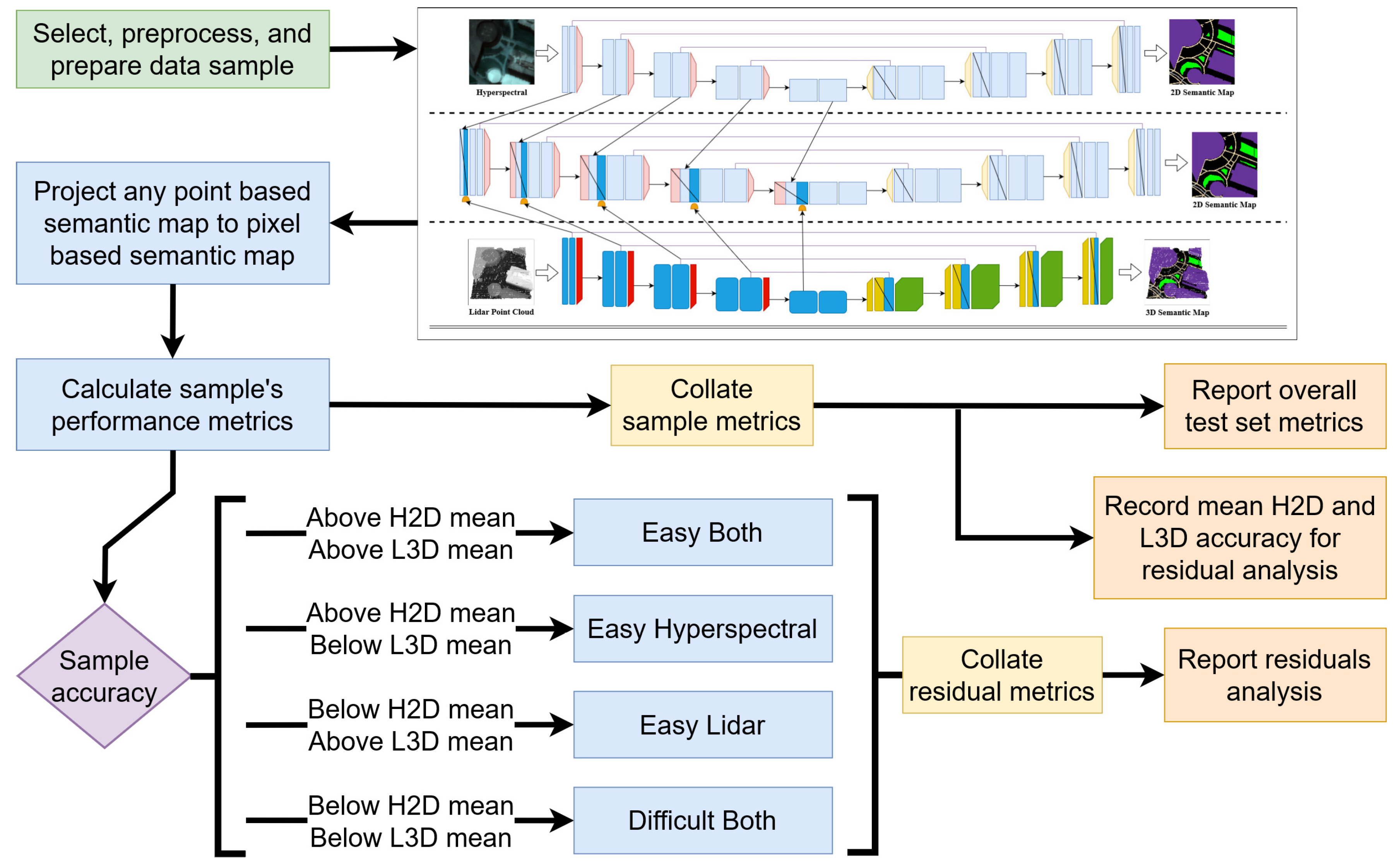
3.1. Residuals Analysis

To further elicit the performance gains of the multimodal models, a more granular metric was warranted. A residuals analysis of the test sample accuracies for all models with respect to the mean test sample accuracy from the H2D and L3D models was performed. First, the mean accuracy for the H2D and L3D models were computed and all test samples were categorized by whether they fall above or below each mean value. Samples falling above the mean value for a given model were categorized as easier to predict (“easy”) for that model and those falling below the mean were categorized as harder to predict (“hard”) for that model. Figure 10 depicts a visualization of the process using histograms to identify the easier and harder samples, which also depicts the easiest and hardest to predict samples for either model.

This categorization process resulted in four distinct categories of multimodal test samples based on the combination of easiness or hardness with respect to both H2D and L3D models:

• Easy Hyperspectral (EH): Contains samples that were easy for H2D to predict accurately but hard for L3D to predict accurately.
• Easy Lidar (EL): Contains samples that were hard for H2D to predict accurately but easy for L3D to predict accurately.
• Easy Both (EB): Contains samples that were easy for both H2D and L3D to predict accurately.
• Difficult Both (DB): Contains samples that were hard for both H2D and L3D to predict accurately.

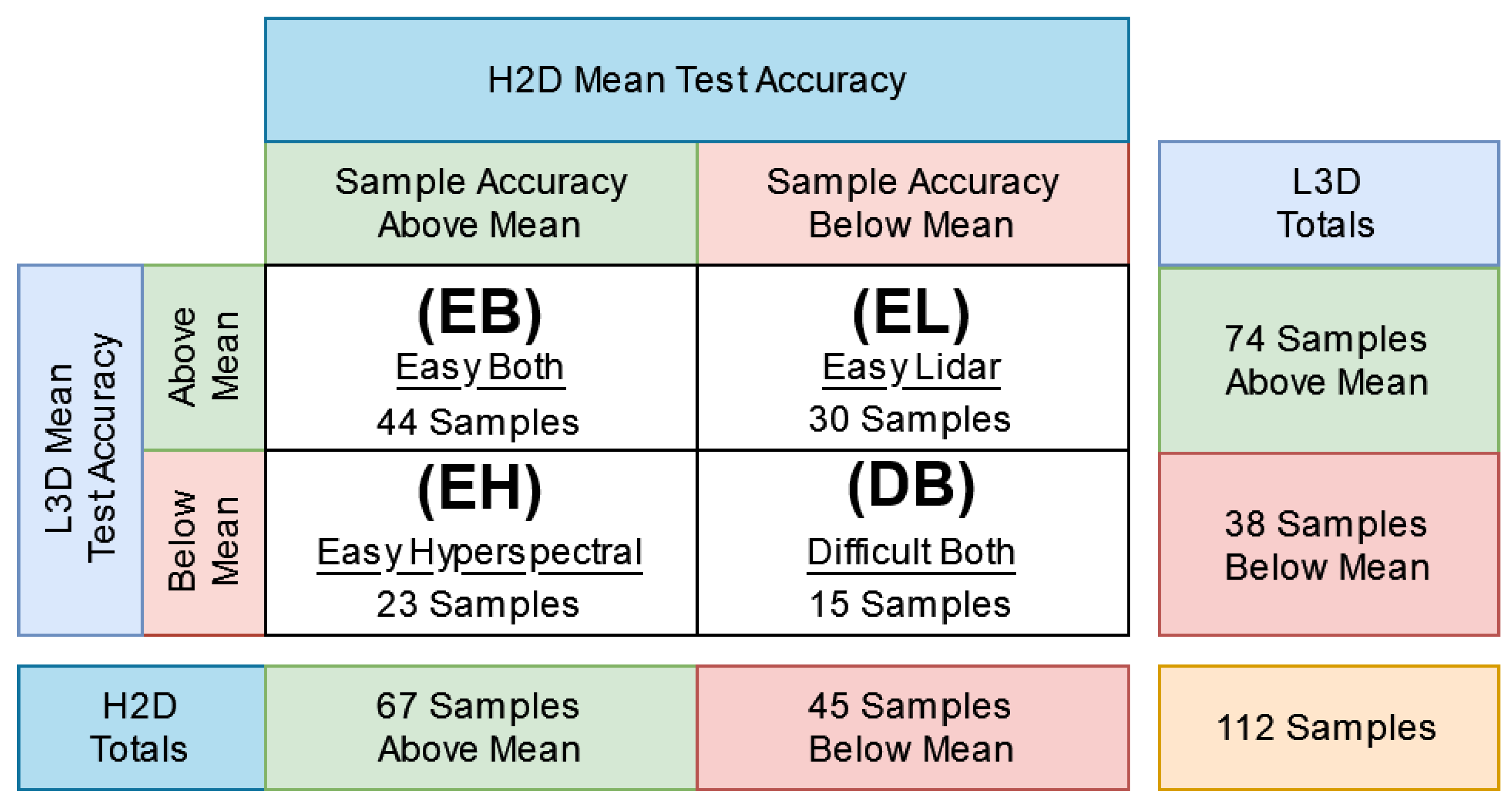
Figure 11 provides a matrix depicting the categorization process and statistics for the test data set samples. The 112 total test samples consisted of 23 EH, 30 EL, 44 EB, and 15 DB sample types. By computing and comparing the mean accuracy of each model against these sample types, it is possible to further outline the performance gains multimodal models made over unimodal models.

3.2. Residuals Analysis Results

In Table 3, it was shown that the unimodal networks achieved the lowest pixel accuracies while the multimodal networks achieved the highest pixel accuracies. However, this does not provide direct evidence that this increased performance is a result of actually fusing information from both modalities rather than more efficiently exploiting a single modality. To investigate this claim, we present the mean test sample accuracy for each model against the four identified sample types as described in Section 3.1 in

Table 4. Each model’s mean test set accuracy with respect to easier- and harder-to-classify samples across both the hyperspectral and lidar modality. Highest mean accuracy per sample type is emboldened.

Architecture	Mean Pixel Accuracy	EH Accuracy	EL Accuracy	EB Accuracy	DB Accuracy
H2D	80.7	89.7	68.3	89.1	67.1
L3D	68.9	30.3	81.2	86.5	52.2
L2D	66.6	32.9	79.4	84.0	41.5
H2D_L3D	83.3	90.6	72.0	89.5	77.1
H2D_L2D	88.6	85.7	89.9	92.0	80.6

. Unsurprisingly, the unimodal networks achieved higher mean test sample accuracy against sample types which are categorized as easy for their given input modality. Consequently, the unimodal networks achieved lower accuracy against samples types which are categorized as hard for their given input modality. For example, the H2D model achieved a higher EH accuracy than both lidar-based unimodal networks L2D and L3D. The lidar-based networks achieved a higher EL accuracy than the hyperspectral-based unimodal network H2D. Together, all three unimodal networks achieved a high EB and low DB accuracy. Thus, the scheme segregates test samples based on the subjective difficulty, as viewed by the unimodal networks collectively.

In Table 4, we find that the multimodal networks collectively outperformed all unimodal networks for the EB and DB test sample types. Furthermore, to some extent, both networks performed either on par with or outperformed all unimodal networks on the EH and EL sample types. These findings provide strong evidence that both multimodal models made their performance gains over unimodal models by fusing information. Note that the unimodal and multimodal architectures share the same components and technology, are provided the same set of test data, and the multimodal networks only have access to weight-frozen unimodal network features. Thus, the only difference between the unimodal and multimodal networks that accounts for the increased mean DB test sample type accuracy is the multimodal models’ ability to fuse information. With all other metrics held constant, there is no other explanation for this increased accuracy against the hardest-to-classify sample type. Had it been the case that the multimodal models only saw improvement in either the EH, EL, or EB sample types, this would indicate that they simply learned a more efficient means of exploiting the corresponding data modality; this could then be traced back to their increased parameter count.

4. Conclusions

The main research goal of this work was the implementation of two proof of concept network architectures which exhibited the strengths of previous neural network-based approaches while improving upon weaknesses. As a result of the composite style architecture, the multimodal networks were able to generate both low- and high-level unimodal and multimodal features without making a trade-off for either. Furthermore, it was assumed that the ingestion of point cloud data and the use of point convolution-based layers would result in a more performant model in both the single and multimodal case. We found this assumption to hold in the unimodal case, but failed for the multimodal case. We are left with the claim that this is a result of the proposed point-to-pixel feature discretization method and its lossy process of discretizing localized groups of point features. This claim is open to future study. In the reported results, we found that regardless of this assumption failing, both multimodal models were able to outperform their unimodal counterparts. Notably, they were able to achieve anywhere from 10 to 40% higher mean accuracy towards hard-to-classify samples (DB) while maintaining performance across other sample types (EH, EL, EB). This result not only provides strong evidence that the composite style architecture generated useful features but also that the act of jointly processing the multimodal data can provide a considerable performance increase over singular processing.

While these results are promising and outlining the novel contributions of this work, future work is still needed. The proposed architectures utilized some of the least complex convolutional network layer technologies for both the pixel and point data. A great deal of research exists into more complex layer types and architectures [20,29,30,31] which may provide additional benefits to both the single and multimodal architectures. It was noted that the data set for this work was modified to produce a more idealized form to separate the effects of more challenging data scenarios such as differing co-, geo-, and temporal registrations and differing viewing geometries and resolutions. Furthermore, while the data set was adequately sized to characterize the network architectures, a larger data set may provide an opportunity to observe the networks’ performance against a larger and more diverse problem instance. The proposed point-to-pixel discretization method needs further study. Many possible alterations exist which may improve its efficacy. For example, the imputation of zero-valued cells during the discretization process may not have yielded meaningful results against this data set, though it may be necessary when working with differing resolutions between modalities. Finally, as noted in Section 1, many works exist which make great effort towards unimodal semantic segmentation. The methods described in these works may be borrowed to further increase the performance of the unimodal network streams. Specifically, the dimensionality reduction and band selection from the hyperspectral modality may provide a considerable pruning of redundant information. This would have a great effect when working with hyperspectral data sets that have hundreds or even thousands of spectral bands.

References

1. Lillesand, T.M.; Kiefer, R.W.; Chipman, J.W. Remote Sensing and Image Interpretation, 7th ed.; John Wiley & Sons, Ltd.: Hoboken, NJ, USA, 2015. [Google Scholar]
2. Lahat, D.; Adali, T.; Jutten, C. Multimodal Data Fusion: An Overview of Methods, Challenges, and Prospects; IEEE: New York, NY, USA, 2015. [Google Scholar] [CrossRef] [Green Version]
3. Rasti, B.; Ghamisi, P.; Plaza, J.; Plaza, A. Fusion of Hyperspectral and LiDAR Data Using Sparse and Low-Rank Component Analysis. IEEE Trans. Geosci. Remote Sens. 2017, 55, 6354–6365. [Google Scholar] [CrossRef] [Green Version]
4. Xia, J.; Yokoya, N.; Iwasaki, A. Fusion of Hyperspectral and LiDAR Data with a Novel Ensemble Classifier. IEEE Geosci. Remote Sens. Lett. 2018, 15, 957–961. [Google Scholar] [CrossRef]
5. Sun, Y.; Zhang, X.; Xin, Q.; Huang, J. Developing a multi-filter convolutional neural network for semantic segmentation using high-resolution aerial imagery and LiDAR data. ISPRS J. Photogramm. Remote Sens. 2018, 143, 3–14. [Google Scholar] [CrossRef]
6. Beger, R.; Gedrange, C.; Hecht, R.; Neubert, M. Data fusion of extremely high resolution aerial imagery and LiDAR data for automated railroad centre line reconstruction. ISPRS J. Photogramm. Remote Sens. 2011, 66, S40–S51. [Google Scholar] [CrossRef]
7. García, M.; Riaño, D.; Chuvieco, E.; Salas, J.; Danson, F.M. Multispectral and LiDAR data fusion for fuel type mapping using Support Vector Machine and decision rules. Remote Sens. Environ. 2011, 115, 1369–1379. [Google Scholar] [CrossRef]
8. Pradhan, B.; Jebur, M.N.; Shafri, H.Z.M.; Tehrany, M.S. Data fusion technique using wavelet transform and taguchi methods for automatic landslide detection from airborne laser scanning data and quickbird satellite imagery. IEEE Trans. Geosci. Remote Sens. 2016, 54, 1610–1622. [Google Scholar] [CrossRef]
9. Li, C.; Tang, X.; Shi, L.; Peng, Y.; Tang, Y. A Two-Staged Feature Extraction Method Based on Total Variation for Hyperspectral Images. Remote Sens. 2022, 14, 302. [Google Scholar] [CrossRef]
10. Xu, Y.; Du, B.; Zhang, L. Multi-source remote sensing data classification via fully convolutional networks and post-classification processing. In Proceedings of the International Geoscience and Remote Sensing Symposium (IGARSS), Valencia, Spain, 22–27 July 2018; pp. 3852–3855. [Google Scholar] [CrossRef]
11. Sukhanov, S.; Budylskii, D.; Tankoyeu, I.; Heremans, R.; Debes, C. Fusion of LiDar, hyperspectral and RGB data for urban land use and land cover classification. In Proceedings of the International Geoscience and Remote Sensing Symposium (IGARSS), Valencia, Spain, 22–27 July 2018; pp. 3864–3867. [Google Scholar] [CrossRef]
12. Mohla, S.; Pande, S.; Banerjee, B.; Chaudhuri, S. FusAtNet: Dual Attention Based SpectroSpatial Multimodal Fusion Network for Hyperspectral and LiDAR Classification. In Proceedings of the IEEE/CVF Conference on Computer Vision and Pattern Recognition (CVPR) Workshops, Seattle, WA, USA, 14–19 June 2020; pp. 92–93. [Google Scholar]
13. Wang, X.; Feng, Y.; Song, R.; Mu, Z.; Song, C. Multi-attentive hierarchical dense fusion net for fusion classification of hyperspectral and LiDAR data. Inf. Fusion 2022, 82, 1–18. [Google Scholar] [CrossRef]
14. Jetley, S.; Lord, N.A.; Lee, N.; Torr, P.H. Learn To Pay Attention. In Proceedings of the 6th International Conference on Learning Representations, ICLR 2018—Conference Track Proceedings, Vancouver, BC, Canada, 30 April–3 May 2018. [Google Scholar] [CrossRef]
15. Mou, L.; Zhu, X.X. Learning to Pay Attention on Spectral Domain: A Spectral Attention Module-Based Convolutional Network for Hyperspectral Image Classification. IEEE Trans. Geosci. Remote Sens. 2020, 58, 110–122. [Google Scholar] [CrossRef]
16. Debes, C.; Merentitis, A.; Heremans, R.; Hahn, J.; Frangiadakis, N.; Van Kasteren, T.; Liao, W.; Bellens, R.; Pizurica, A.; Gautama, S.; et al. Hyperspectral and LiDAR data fusion: Outcome of the 2013 GRSS data fusion contest. IEEE J. Sel. Top. Appl. Earth Obs. Remote Sens. 2014, 7, 2405–2418. [Google Scholar] [CrossRef]
17. Piramanayagam, S.; Saber, E.; Schwartzkopf, W.; Koehler, F. Supervised Classification of Multisensor Remotely Sensed Images Using a Deep Learning Framework. Remote Sens. 2018, 10, 1429. [Google Scholar] [CrossRef] [Green Version]
18. Karpathy, A.; Toderici, G.; Shetty, S.; Leung, T.; Sukthankar, R.; Li, F.F. Large-scale video classification with convolutional neural networks. In Proceedings of the IEEE Computer Society Conference on Computer Vision and Pattern Recognition, Columbus, OH, USA, 23–28 June 2014; pp. 1725–1732. [Google Scholar] [CrossRef] [Green Version]
19. Guo, Y.; Wang, H.; Hu, Q.; Liu, H.; Liu, L.; Bennamoun, M. Deep Learning for 3D Point Clouds: A Survey. arXiv 2019, arXiv:1912.12033. [Google Scholar] [CrossRef] [PubMed]
20. Thomas, H.; Qi, C.R.; Deschaud, J.E.; Marcotegui, B.; Goulette, F.; Guibas, L.J. KPConv: Flexible and Deformable Convolution for Point Clouds. In Proceedings of the IEEE International Conference on Computer Vision, Seoul, Korea, 27–28 October 2019; pp. 6410–6419. [Google Scholar]
21. Xu, Y.; Du, B.; Zhang, L.; Cerra, D.; Pato, M.; Carmona, E.; Prasad, S.; Yokoya, N.; Hansch, R.; Le Saux, B. Advanced multi-sensor optical remote sensing for urban land use and land cover classification: Outcome of the 2018 ieee grss data fusion contest. IEEE J. Sel. Top. Appl. Earth Obs. Remote Sens. 2019, 12, 1709–1724. [Google Scholar] [CrossRef]
22. Hong, D.; Chanussot, J.; Yokoya, N.; Kang, J.; Zhu, X.X. Learning-Shared Cross-Modality Representation Using Multispectral-LiDAR and Hyperspectral Data. IEEE Geosci. Remote Sens. Lett. 2020, 17, 1470–1474. [Google Scholar] [CrossRef] [Green Version]
23. Cerra, D.; Pato, M.; Carmona, E.; Azimi, S.M.; Tian, J.; Bahmanyar, R.; Kurz, F.; Vig, E.; Bittner, K.; Henry, C.; et al. Combining deep and shallow neural networks with ad hoc detectors for the classification of complex multi-modal urban scenes. In Proceedings of the International Geoscience and Remote Sensing Symposium (IGARSS), Valencia, Spain, 22–27 July 2018; pp. 3856–3859. [Google Scholar] [CrossRef] [Green Version]
24. Fang, S.; Quan, D.; Wang, S.; Zhang, L.; Zhou, L. A two-branch network with semi-supervised learning for hyperspectral classification. In Proceedings of the International Geoscience and Remote Sensing Symposium (IGARSS), Valencia, Spain, 22–27 July 2018; pp. 3860–3863. [Google Scholar] [CrossRef]
25. Ronneberger, O.; Fischer, P.; Brox, T. U-Net: Convolutional Networks for Biomedical Image Segmentation. arXiv 2015, arXiv:1505.04597. [Google Scholar]
26. Cao, F.; Yang, Z.; Ren, J.; Jiang, M.; Ling, W.K. Does Normalization Methods Play a Role for Hyperspectral Image Classification? arXiv 2017, arXiv:1710.02939. [Google Scholar]
27. Paszke, A.; Gross, S.; Massa, F.; Lerer, A.; Bradbury, J.; Chanan, G.; Killeen, T.; Lin, Z.; Gimelshein, N.; Antiga, L.; et al. PyTorch: An Imperative Style, High-Performance Deep Learning Library. In Advances in Neural Information Processing Systems 32; Wallach, H., Larochelle, H., Beygelzimer, A., d’Alché-Buc, F., Fox, E., Garnett, R., Eds.; Curran Associates, Inc.: Red Hook, NY, USA, 2019; pp. 8024–8035. [Google Scholar]
28. Fey, M. Pytorch_Scatter. 2021. Available online: https://github.com/rusty1s/pytorch_scatter/releases/tag/2.0.9 (accessed on 15 November 2021).
29. Simonyan, K.; Zisserman, A. Very Deep Convolutional Networks for Large-Scale Image Recognition. arXiv 2014, arXiv:1409.1556. [Google Scholar]
30. Szegedy, C.; Liu, W.; Jia, Y.; Sermanet, P.; Reed, S.; Anguelov, D.; Erhan, D.; Vanhoucke, V.; Rabinovich, A. Going deeper with convolutions. In Proceedings of the IEEE Computer Society Conference on Computer Vision and Pattern Recognition, Boston, MA, USA, 7–12 June 2015; pp. 1–9. [Google Scholar] [CrossRef] [Green Version]
31. He, K.; Zhang, X.; Ren, S.; Sun, J. Deep Residual Learning for Image Recognition. In Proceedings of the IEEE Conference on Computer Vision and Pattern Recognition (CVPR), Las Vegas, NV, USA, 27–30 June 2016; pp. 770–778. [Google Scholar]
Figure 1. Pictorial representation of pixel and point convolutions. (Left) Pixel features localized by pixel locations are generated by convolving a set of learned kernels over the previous layer’s feature set. (Right) Point features localized by point locations are generated by convolving a set of learned kernels over the previous layer’s feature set. Pixel convolution is seen as a special case of point convolution where the influence of each kernel weight is uniform at each pixel. Reprinted, with permission, from [20]. ©2022 IEEE.
Remotesensing 14 02113 g001
Figure 2. Pictorial representation of residual issues resulting from underdetermined transfer of labels from the pixel to point domain. (Left) The 128 × 128 m 2 area of labeled lidar point cloud depicting multiple buildings along with surrounding foliage and roadways; (Right) Selected area of scene in which points below overhanging foliage are incorrectly labeled as foliage. Note: Unclassified point coloring changed from black to light gray for easier visualization.
Remotesensing 14 02113 g002
Figure 3. Altered GRSS18 data set utilized in this work. (Top Left) Complete hyperspectral image used in this work, originally a subset of GRSS18 hyperspectral image. (Top Right) Complete lidar point cloud used in this work, originally Channel 1 of the GRSS18 multispectral lidar. Coloring of points based on height above ground. (Bottom Left) Semantic pixel map of superclass values over the hyperspectral image. (Bottom Right) Labeled lidar point cloud used for training point convolution-based networks.
Remotesensing 14 02113 g003
Figure 4. Three example multimodal data samples comprised of co-registered (Left) hyperspectral, (Center) lidar point cloud, and (Right) a semantic point map. The semantic point map is provided to better visualize raw point cloud context.
Remotesensing 14 02113 g004
Figure 5. Pixel convolution-based networks. (Top) H2D ingesting raw hyperspectral data and predicting a 2D semantic map. (Bottom) L2D ingesting a lidar DSM and predicting a 2D semantic map. (Center) H2D_L2D ingesting low- and high-level unimodal hyperspectral and lidar features via fusion connections from H2D and L2D and predicting a 2D semantic map. H2D_L2D is constructed as a composite style fusion architecture inspired by [17].
Remotesensing 14 02113 g005
Figure 6. Point convolution-based networks, H2D is pictured again. (Top) H2D ingesting raw hyperspectral data and predicting a 2D semantic map. (Bottom) L3D ingesting a lidar point cloud and predicting a 3D semantic map utilizing KPConv layers for processing as originally described by [20]. (Center) H2D_L3D ingesting low- and high-level unimodal hyperspectral and lidar features via fusion connections from H2D and L3D and predicting a 2D semantic map. H2D_L3D is constructed as a composite style fusion architecture inspired by [17].
Remotesensing 14 02113 g006
Figure 7. Pictorial representation of a novel method of 3D point feature discretization. (Left) Hyperspectral pixel and lidar point feature tensors for any given encoding section of H2D_L3D (light red) and L3D (blues). (Center) The bucketization of original point locations into a grid with the same size as the FsNet receptive field, the gather–scatter of point features into each cell, the reduction in point features for each cell, and the final discretization into a rectangular tensor. (Right) The concatenation-based fusion of pixel features and discretized point features.
Remotesensing 14 02113 g007
Figure 8. Overall workflow of the methodology from data to decision products. First, the GRSS18 data set [21] is modified and preprocessed to produce training, validation, and testing multimodal samples. A model from each of the five network architectures described is then trained (L2D and H2D_L2D not pictured). The predicted semantic maps are post processed; sample metrics are calculated and collated into overall test set metrics. Finally, the results of H2D and L3D are used to perform the residual analysis. Overview and motivation of residual analysis provided in Section 3.1.
Remotesensing 14 02113 g008
Figure 9. Combined test sample predictions over the entire test set area for all models. (Row 1, Column 1) False color hyperspectral image of test set area. (R1C2) Ground truth labeling of test set area. (R2C1) H2D prediction. (R3C1) L3D prediction in point cloud format. (R4C1) L3D prediction in pixel format. (R2C2) L2D prediction. (R3C2) H2D_L3D prediction. (R4C2) H2D_L2D prediction.
Remotesensing 14 02113 g009
Figure 10. Histograms of test set accuracy over individual samples observed from H2D and L3D and examples of sample performance. (Top) H2D histogram along with the lowest and highest accuracy samples. (Bottom) L3D histogram along with the lowest and highest accuracy samples. Lowest and highest accuracy samples are colored by correct pixels/points (green), incorrect pixels/points (red), and masked unlabeled pixels/points (light gray).
Remotesensing 14 02113 g010
Figure 11. Categorization matrix for test samples. The mean test set accuracy for the H2D and L3D models are calculated. Each test sample is then categorized into one of four types based on the pixel accuracy achieved by both H2D and L3D against the sample. Test sample accuracies above the model mean are categorized as “easy”, whilst accuracies below the model mean are categorized as “hard”.
Remotesensing 14 02113 g011