
Thaw Settlement Monitoring and Active Layer Thickness Retrieval Using Time Series COSMO-SkyMed Imagery in Iqaluit Airport


 ,
,  ,
,  , ,
, ,  and
and
Abstract
:1. Introduction
2. Materials and Methods
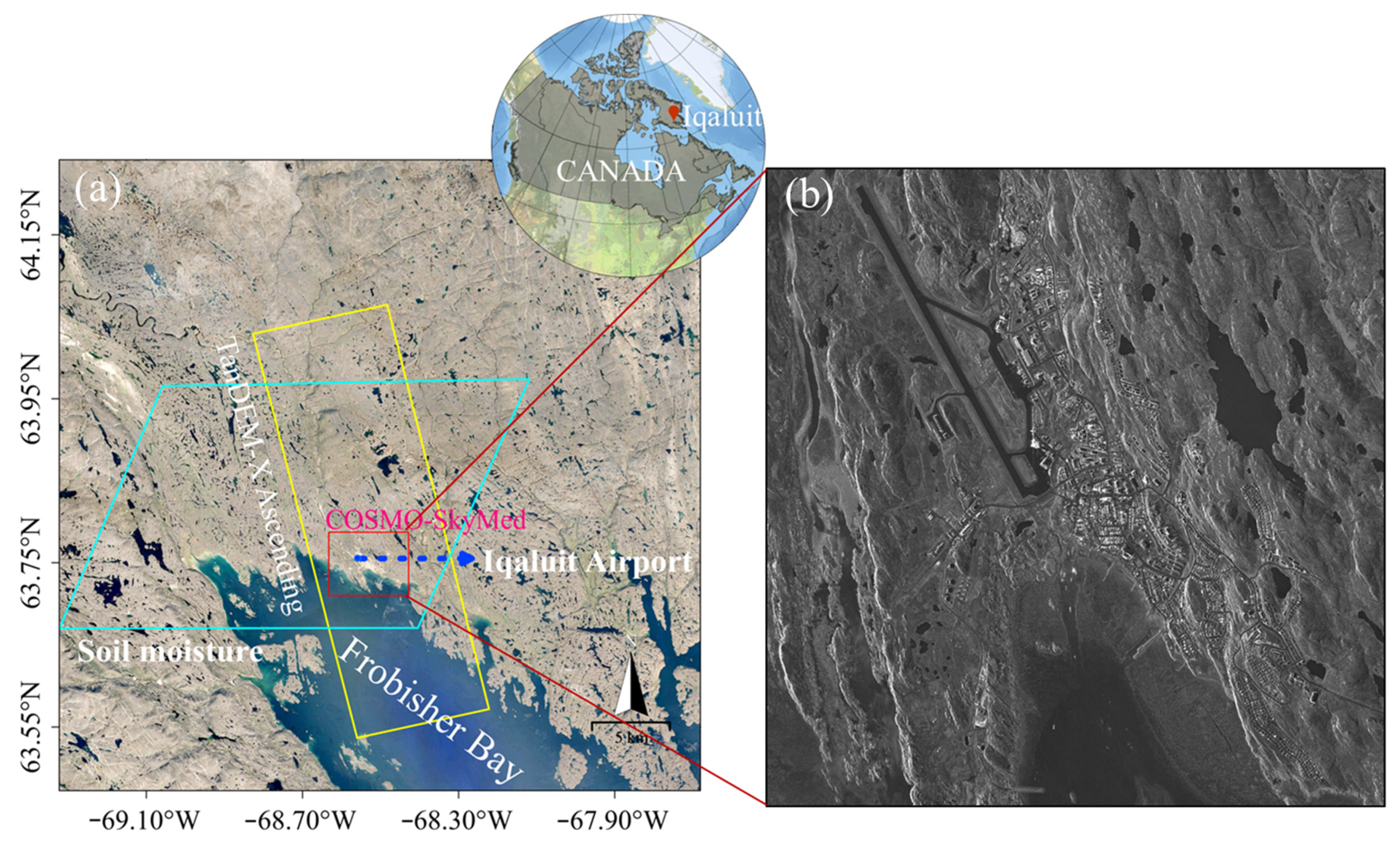
2.1. Study Area
2.2. Dataset
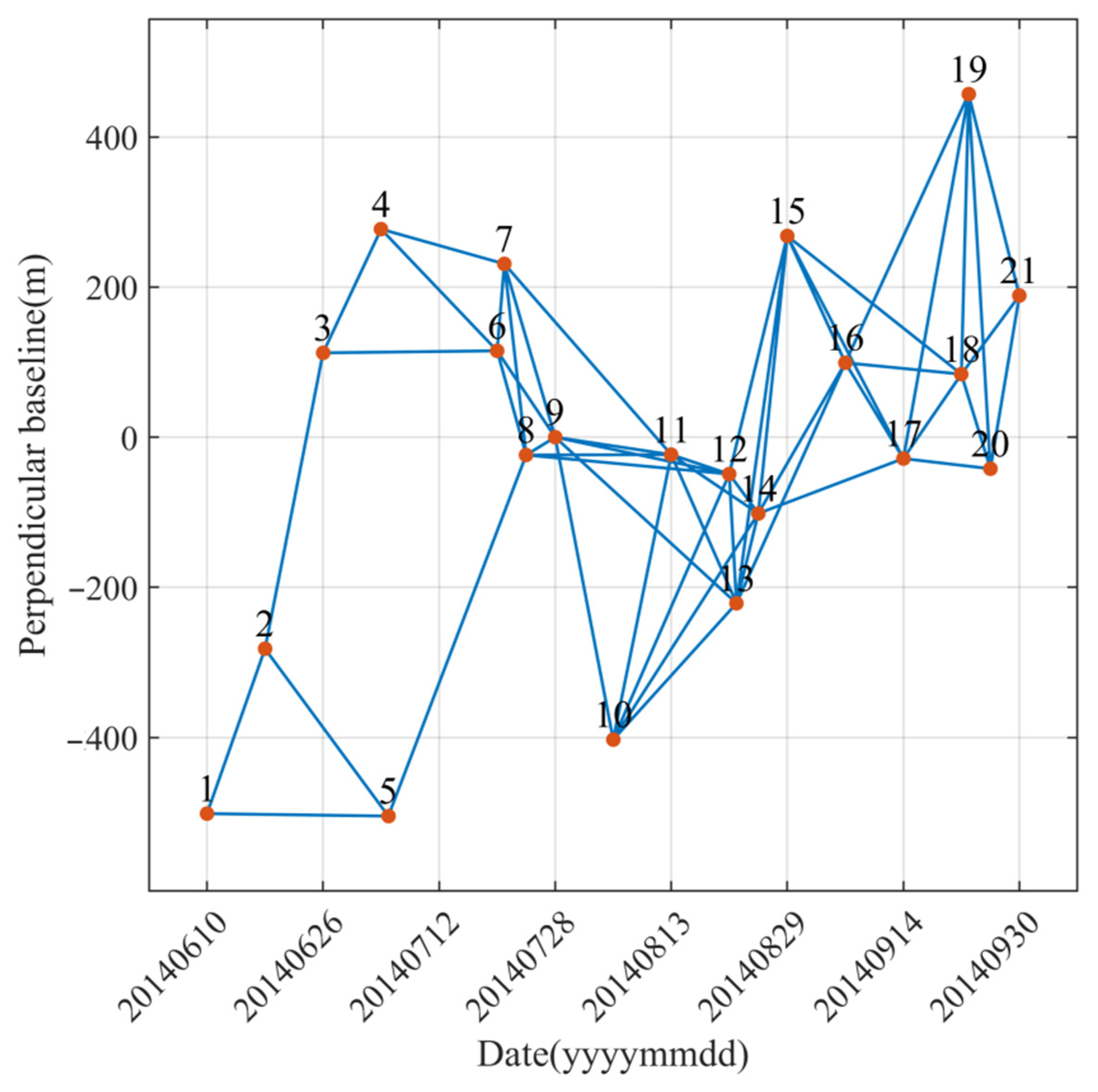
2.2.1. SAR Data
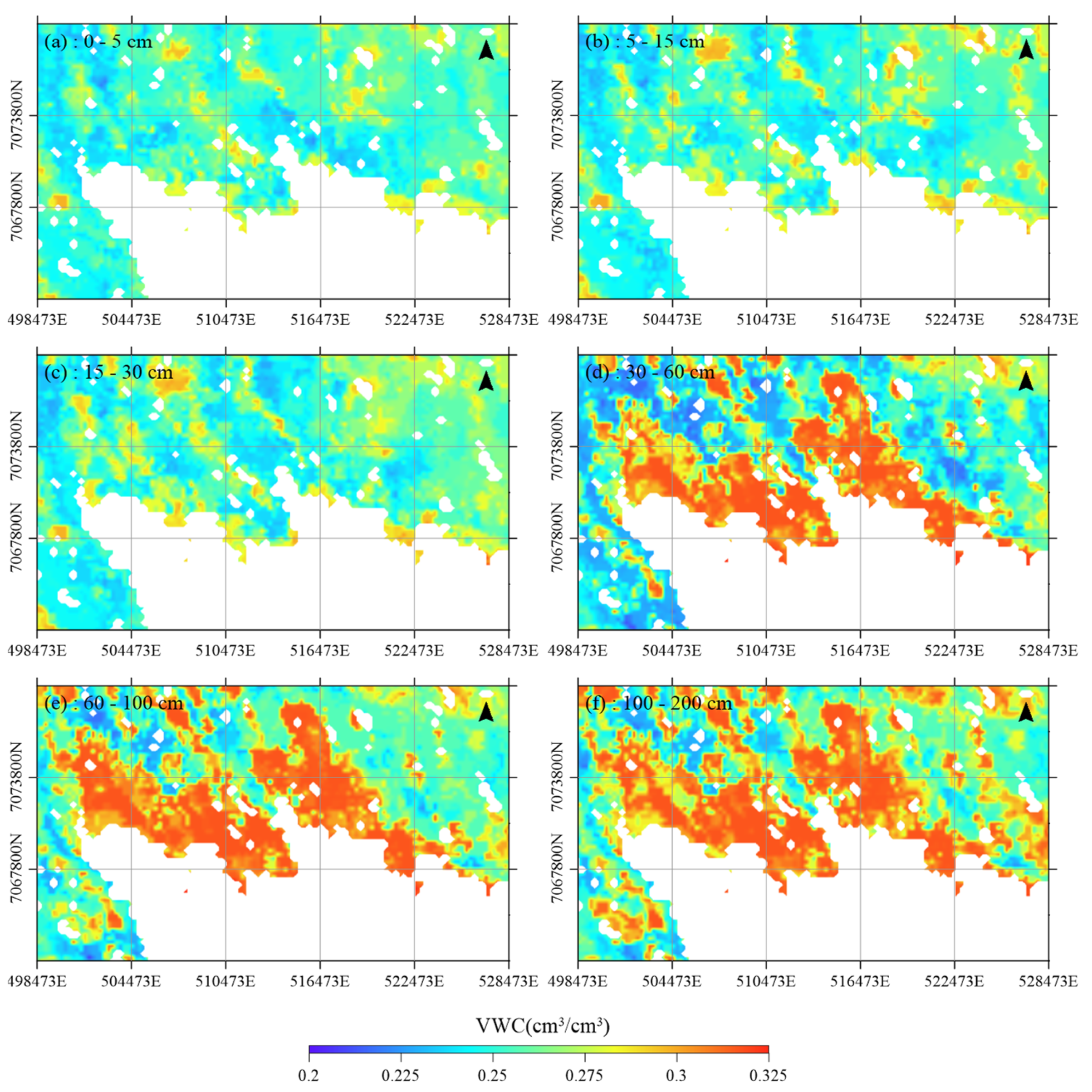
2.2.2. Soil Moisture Data
2.3. Methodology
2.3.1. Subsidence Observation from CSK Spotlight SAR Images
2.3.2. ALT Estimation
- Soil in an unsaturated state
- Soil in a saturated state
- Soil in an oversaturated state
3. Results
3.1. Deformation Results
3.2. Estimated ALT Results
4. Analysis and Discussion
4.1. Comparison of Subsidence with GPS Data and Thaw Tubes
4.2. ALT Validation with Thermistor Cable Measurements
4.3. Uneven Trend of Subsidence and ALT along the Runway
4.4. ALTs under Infrastructure and Natural Ground
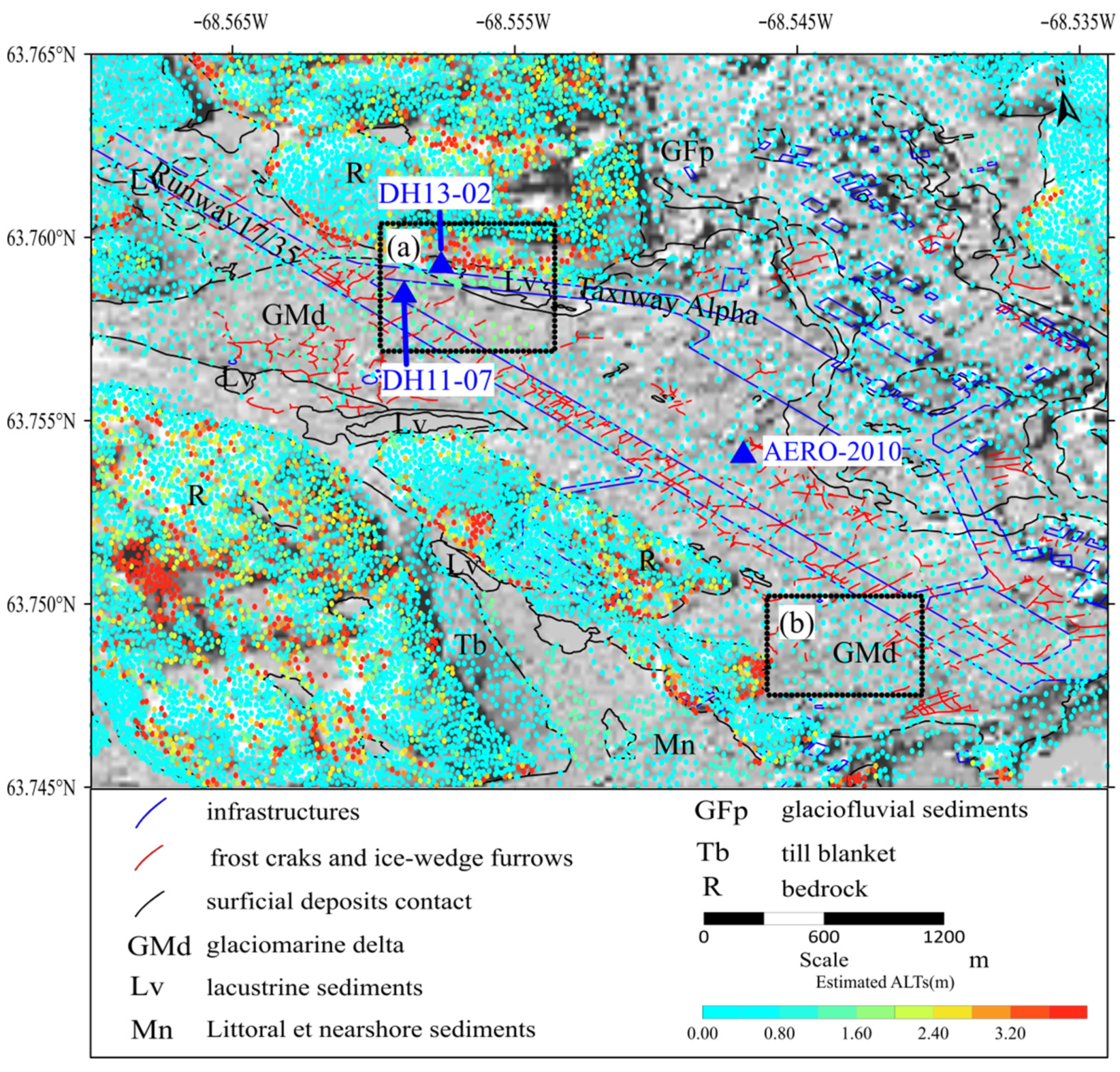
4.5. Relation between ALT and Geology
4.6. Limitations
5. Conclusions
Author Contributions
Funding
Institutional Review Board Statement
Informed Consent Statement
Data Availability Statement
Acknowledgments
Conflicts of Interest
References
- Obu, J. How Much of the Earth’s Surface Is Underlain by Permafrost? J. Geophys. Res. Earth Surf. 2021, 126, e2021JF006123. [Google Scholar] [CrossRef]
- Streletskiy, D.A.; Suter, L.J.; Shiklomanov, N.I.; Porfiriev, B.N.; Eliseev, D.O. Assessment of Climate Change Impacts on Buildings, Structures and Infrastructure in the Russian Regions on Permafrost. Environ. Res. Lett. 2019, 14, 025003. [Google Scholar] [CrossRef]
- Streletskiy, D.; Anisimov, O.; Vasiliev, A. Permafrost Degradation. In Snow and Ice-Related Hazards, Risks and Disasters; Elsevier: Amsterdam, The Netherlands, 2015; pp. 303–344. [Google Scholar]
- Schneider von Deimling, T.; Lee, H.; Ingeman-Nielsen, T.; Westermann, S.; Romanovsky, V.; Lamoureux, S.; Walker, D.A.; Chadburn, S.; Trochim, E.; Cai, L.; et al. Consequences of Permafrost Degradation for Arctic Infrastructure–Bridging the Model Gap between Regional and Engineering Scales. Cryosphere 2021, 15, 2451–2471. [Google Scholar] [CrossRef]
- Karjalainen, O.; Aalto, J.; Luoto, M.; Westermann, S.; Romanovsky, V.E.; Nelson, F.E.; Etzelmüller, B.; Hjort, J. Circumpolar Permafrost Maps and Geohazard Indices for Near-Future Infrastructure Risk Assessments. Sci. Data 2019, 6, 1–16. [Google Scholar] [CrossRef] [Green Version]
- Niu, F.; Yin, G.; Luo, J.; Lin, Z.; Liu, M. Permafrost Distribution along the Qinghai-Tibet Engineering Corridor, China Using High-Resolution Statistical Mapping and Modeling Integrated with Remote Sensing and GIS. Remote Sens. 2018, 10, 215. [Google Scholar] [CrossRef] [Green Version]
- Chen, F.; Lin, H.; Li, Z.; Chen, Q.; Zhou, J. Interaction between Permafrost and Infrastructure along the Qinghai–Tibet Railway Detected via Jointly Analysis of C- and L-Band Small Baseline SAR Interferometry. Remote Sens. Environ. 2012, 123, 532–540. [Google Scholar] [CrossRef]
- Rickard, W.; Brown, J. The Performance of a Frost-Tube for the Determination of Soil Freezing and Thawing Depths. Soil Sci. 1972, 113, 149–154. [Google Scholar] [CrossRef]
- Grasmueck, M.; Weger, R.; Horstmeyer, H. Full-Resolution 3D GPR Imaging. Geophysics 2005, 70, K12–K19. [Google Scholar] [CrossRef]
- Park, B.; Kim, J.; Lee, J.; Kang, M.-S.; An, Y.-K. Underground Object Classification for Urban Roads Using Instantaneous Phase Analysis of Ground-Penetrating Radar (GPR) Data. Remote Sens. 2018, 10, 1417. [Google Scholar] [CrossRef] [Green Version]
- Jonard, F.; Weihermüller, L.; Schwank, M.; Jadoon, K.Z.; Vereecken, H.; Lambot, S. Estimation of Hydraulic Properties of a Sandy Soil Using Ground-Based Active and Passive Microwave Remote Sensing. IEEE Trans. Geosci. Remote Sens. 2015, 53, 3095–3109. [Google Scholar] [CrossRef]
- Goodrich, L.E. The Influence of Snow Cover on the Ground Thermal Regime. Can. Geotech. J. 1982, 19, 421–432. [Google Scholar] [CrossRef] [Green Version]
- Nelson, P.; Oades, J. Organic Matter, Sodicity and Soil Structure. In Sodic Soils: Distribution, Properties, Management and Environmental Consequences; Topics in Sustainable Agronomy; Oxford University Press: Oxford, UK, 1998; pp. 51–75. [Google Scholar]
- Vuik, C. Some Historical Notes about the Stefan Problem; Delft University of Technology: Delft, The Netherlands, 1993. [Google Scholar]
- Chen, R.H.; Tabatabaeenejad, A.; Moghaddam, M. Retrieval of Permafrost Active Layer Properties Using Time-Series P-Band Radar Observations. IEEE Trans. Geosci. Remote Sens. 2019, 57, 6037–6054. [Google Scholar] [CrossRef]
- Li, Z.; Zhao, R.; Hu, J.; Wen, L.; Feng, G.; Zhang, Z.; Wang, Q. InSAR Analysis of Surface Deformation over Permafrost to Estimate Active Layer Thickness Based on One-Dimensional Heat Transfer Model of Soils. Sci. Rep. 2015, 5, 1–9. [Google Scholar] [CrossRef] [PubMed]
- Liu, L.; Schaefer, K.; Zhang, T.; Wahr, J. Estimating 1992–2000 Average Active Layer Thickness on the Alaskan North Slope from Remotely Sensed Surface Subsidence. J. Geophys. Res. Earth Surf. 2012, 117. [Google Scholar] [CrossRef]
- Chang, T.; Han, J.; Li, Z.; Wen, Y.; Hao, T.; Lu, P.; Li, R. Active Layer Thickness Retrieval Over the Qinghai-Tibet Plateau from 2000 TO 2020 Based on Insar-Measured Subsidence and Multi-Layer Soil Moisture. ISPRS-Int. Arch. Photogramm. Remote Sens. Spat. Inf. Sci. 2021, 43, 437–442. [Google Scholar] [CrossRef]
- Rouyet, L.; Liu, L.; Strand, S.M.; Christiansen, H.H.; Lauknes, T.R.; Larsen, Y. Seasonal InSAR Displacements Documenting the Active Layer Freeze and Thaw Progression in Central-Western Spitsbergen, Svalbard. Remote Sens. 2021, 13, 2977. [Google Scholar] [CrossRef]
- Wang, C.; Zhang, Z.; Zhang, H.; Zhang, B.; Tang, Y.; Wu, Q. Active Layer Thickness Retrieval of Qinghai–Tibet Permafrost Using the TerraSAR-X InSAR Technique. IEEE J. Sel. Top. Appl. Earth Obs. Remote Sens. 2018, 11, 4403–4413. [Google Scholar] [CrossRef]
- Clayton, L.K.; Schaefer, K.; Battaglia, M.J.; Bourgeau-Chavez, L.; Chen, J.; Chen, R.H.; Chen, A.; Bakian-Dogaheh, K.; Grelik, S.; Jafarov, E. Active Layer Thickness as a Function of Soil Water Content. Environ. Res. Lett. 2021, 16, 055028. [Google Scholar] [CrossRef]
- Zhang, X.; Zhang, H.; Wang, C.; Tang, Y.; Zhang, B.; Wu, F.; Wang, J.; Zhang, Z. Active Layer Thickness Retrieval Over the Qinghai-Tibet Plateau Using Sentinel-1 Multitemporal InSAR Monitored Permafrost Subsidence and Temporal-Spatial Multilayer Soil Moisture Data. IEEE Access 2020, 8, 84336–84351. [Google Scholar] [CrossRef]
- Luo, D.; Jin, H.; Wu, Q.; Bense, V.F.; He, R.; Ma, Q.; Gao, S.; Jin, X.; Lü, L. Thermal Regime of Warm-Dry Permafrost in Relation to Ground Surface Temperature in the Source Areas of the Yangtze and Yellow Rivers on the Qinghai-Tibet Plateau, SW China. Sci. Total Environ. 2018, 618, 1033–1045. [Google Scholar] [CrossRef]
- Klene, A.E.; Nelson, F.E. Urban Geocryology: Mapping Urban–Rural Contrasts in Active-Layer Thickness, Barrow Peninsula, Northern Alaska. Ann. Am. Assoc. Geogr. 2019, 109, 1394–1414. [Google Scholar] [CrossRef]
- Taber, S. The Mechanics of Frost Heaving. J. Geol. 1930, 38, 303–317. [Google Scholar] [CrossRef]
- Beskow, G. Soil Freezing and Frost Heaving with Special Application to Roads and Railroads; Osterberg, J.O., Translator; The Swedish Geological Society, C, no. 375, Year Book no. 3; Technological Institute, Northwestern University: Evanston, IL, USA, 1935. [Google Scholar]
- Black, P.B.; Hardenberg, M.J. Historical Perspectives in Frost Heave Research: The Early Works of S. Taber and G. Beskow; Special Report (Cold Regions Research and Engineering Laboratory (U.S.)); Cold Regions Research and Engineering Laboratory, Engineer Research and Development Center: Vicksburg, MS, USA, 1991; pp. 23–91. [Google Scholar]
- Dash, J.G.; Rempel, A.W.; Wettlaufer, J.S. The Physics of Premelted Ice and Its Geophysical Consequences. Rev. Modern Phys. 2006, 78, 695–741. [Google Scholar] [CrossRef] [Green Version]
- Yanagiya, K.; Furuya, M. Post-wildfire surface deformation near Batagay, Eastern Siberia, detected by l-band and c-band InSAR. J. Geophys. Res. Earth Surface. 2020, 125, e2019JF005473. [Google Scholar] [CrossRef]
- Liu, G.X.; Buckley, S.M.; Ding, X.L.; Chen, Q.; Luo, X.J. Estimating Spatiotemporal Ground Deformation With Improved Persistent-Scatterer Radar Interferometry. IEEE Trans. Geosci. Remote Sens. 2009, 47, 3209–3219. [Google Scholar] [CrossRef]
- Liu, G.; Jia, H.; Zhang, R.; Zhang, H.; Jia, H.; Yu, B.; Sang, M. Exploration of Subsidence Estimation by Persistent Scatterer InSAR on Time Series of High Resolution TerraSAR-X Images. IEEE J. Sel. Top. Appl. Earth Obs. Remote Sens. 2010, 4, 159–170. [Google Scholar] [CrossRef]
- Murton, J.B. Permafrost and Climate Change. In Climate Change; Elsevier: Amsterdam, The Netherlands, 2021; pp. 281–326. [Google Scholar]
- Allard, M.; Doyon, J.; Oldenborger, G.A.; Sladen, W.; LeBlanc, A.-M.; Mathon-Dufour, V.; L’Hérault, E.; Mate, D. Surficial Geology, Iqaluit, Nunavut; Geological Survey of Canada: Ottawa, ON, Canada, 2012.
- International Permafrost Association. Frozen Ground-The News Bulletin of the International Permafrost Association, No. 25. Frozen Ground 2001, 25. [Google Scholar]
- Hengl, T.; Mendes de Jesus, J.; Heuvelink, G.B.; Ruiperez Gonzalez, M.; Kilibarda, M.; Blagotić, A.; Shangguan, W.; Wright, M.N.; Geng, X.; Bauer-Marschallinger, B.; et al. SoilGrids250m: Global Gridded Soil Information Based on Machine Learning. PLoS One 2017, 12, e0169748. [Google Scholar] [CrossRef] [Green Version]
- Ferretti, A.; Prati, C.; Rocca, F. Permanent scatterers in SAR interferometry. IEEE Trans. Geosci. Remote Sens. 2001, 39, 8–20. [Google Scholar] [CrossRef]
- Lanari, R.; Mora, O.; Manunta, M.; Mallorquí, J.J.; Berardino, P.; Sansosti, E. A small-baseline approach for investigating deformations on full-resolution differential SAR interferograms. IEEE Trans. Geosci. Remote Sens 2004, 42, 1377–1386. [Google Scholar]
- Huang, N.E.; Shen, Z.; Long, S.R.; Wu, M.C.; Shih, H.H.; Zheng, Q.; Yen, N.C.; Tung, C.C.; Liu, H.H. The Empirical Mode Decomposition and the Hilbert Spectrum for Nonlinear and Non-Stationary Time Series Analysis. Proc. Math. Phys. Eng. Sci. 1998, 454, 903–995. [Google Scholar] [CrossRef]
- Watson, G.; Slusarchuk, W.; Rowley, R. Determination of Some Frozen and Thawed Properties of Permafrost Soils. Can. Geotech. J. 1973, 10, 592–606. [Google Scholar] [CrossRef]
- Ping, H.; Guodong, C.; Chengsong, Y. The Evaluation of Thawing-Settlement Coefficient of Frozen Soils. J. Glaciol. Geocryol. 2003, 25, 608–613. [Google Scholar]
- Xifa, Z.; Ji, C.; Dongqing, Z. Application of Thawing Settlement Coefficient to the Research on the Roadbed Frost Damage of Freeway in Seasonal Frost Region. J. Glaciol. Geocryol. 2002, 24, 634–638. [Google Scholar]
- Brooks, H.; Doré, G.; Lemieux, C. Quantitative Risk Assessment of the Iqaluit International Airport, Iqaluit, Nu-navut.; Prepared for The Northern Transportation Adaptation Initiative from Transport Canada; Université Laval: Québec, QC, Canada, 2017; p. 53. [Google Scholar]
- Blewitt, G.; Hammond, W.C.; Kreemer, C. Harnessing the GPS data explosion for interdisciplinary science. Eos 2018, 99, 485. [Google Scholar] [CrossRef]
- LeBlanc, A.M.; Short, N.; Oldenborger, G.A.; Mathon-Dufour, V.; Allard, M. Geophysical Investigation and InSAR Mapping of Permafrost and Ground Movement at the Iqaluit Airport. In Cold Regions Engineering 2012: Sustainable Infrastructure Development in a Changing Cold Environment; American Society of Civil Engineers: Reston, VA, USA, 2012; pp. 644–654. [Google Scholar]
- Short, N.; LeBlanc, A.M.; Sladen, W.; Oldenborger, G.; Mathon-Dufour, V.; Brisco, B. RADARSAT-2 D-InSAR for ground displacement in permafrost terrain, validation from Iqaluit Airport, Baffin Island, Canada. Remote Sens. Environ. 2014, 141, 40–51. [Google Scholar] [CrossRef]
- Short, N. RADARSAT Constellation Mission DInSAR Potential in Permafrost Terrain; Natural Resources Canada: Ottawa, ON, Canada, 2017. [CrossRef]
- Mathon-Dufour, V.; Allard, M.; Leblanc, A.; L’Hérault, E.; Oldenborger, G.; Sladen, W. Mapping Surficial Geology and Assessment of Permafrost Conditions under the Iqaluit Airport, Nunavut, Canada. In Proceedings of the AGU Fall Meeting Abstracts, San Francisco, CA, USA, 3 December 2012. [Google Scholar]
- LeBlanc, A.M.; Mathon-Dufour, V.; Allard, M.; Oldenborger, G.A.; Short, N.; L’Hérault, E.; Sladen, W.E. Permafrost characterization at the Iqaluit International Airport, Nunavut, in support of decision-making and planning. Summ. Act. 2012, 131–142. [Google Scholar]
- Rémillard, A.M.; Hétu, B.; Bernatchez, P.; Buylaert, J.-P.; Murray, A.S.; St-Onge, G.; Geach, M. Chronology and Palaeoenvironmental Implications of the Ice-Wedge Pseudomorphs and Composite-Wedge Casts on the Magdalen Islands (Eastern Canada). Boreas 2015, 44, 658–675. [Google Scholar] [CrossRef]
- Mathon-Dufour, V. Caractérisation Du Pergélisol En Vue de La Réfection et de l’adaptation Aux Changements Climatiques de L’aéroport D’Iqaluit; Université Laval: Québec, QC, Canada, 2014. [Google Scholar]
- LeBlanc, A.M.; Short, N.; Mathon-Dufour, V.; Allard, M.; Tremblay, T.; Oldenborger, G.A.; Chartrand, J. DInSAR seasonal surface displacement in built and natural permafrost environments, Iqaluit, Nunavut, Canada. In Proceedings of the GEO, Québec, QC, Canada, 25–28 February 2015; pp. 20–23. [Google Scholar]
- Martini, I.P. Deglaciation Stages of the Laurentide Ice Sheet in Canada and Related Glaciomarine and Glaciolacustrine Deposits. Rev. Sel. Features 2007. Available online: https://minerva.usc.es/xmlui/handle/10347/3757 (accessed on 26 January 2022).
- Hillier, S. Erosion, Sedimentation and Sedimentary Origin of Clays. In Origin and mineralogy of clays. In Origin and Mineralogy of Clays; Springer: Berlin/Heidelberg, Germany, 1995; pp. 162–219. [Google Scholar]


| Date | Date | Date |
|---|---|---|
| 10 June 2014 | 24 July 2014 | 29 August 2014 |
| 18 June 2014 | 28 July 2014 | 6 September 2014 |
| 26 June 2014 | 5 August 2014 | 14 September 2014 |
| 4 July 2014 | 13 August 2014 | 22 September 2014 |
| 5 July 2014 | 21 August 2014 | 23 September 2014 |
| 20 July 2014 | 22 August 2014 | 26 September 2014 |
| 21 July 2014 | 25 August 2014 | 30 September 2014 |
| Sediment Type | |||
|---|---|---|---|
| R (bedrock) | 0.42 | 2.4 | 2.75 |
| Other sediments | 0.42 | 1.9 | 2.65 |
| GPS Station | Coordinates |
|---|---|
| IQAC | 63.737 N, −68.540 W |
| IQAL | 63.756 N, −68.510 W |
| Thaw Tubes | In Situ Subsidence (cm) | Subsidence from FCNInSAR (cm) | Year |
|---|---|---|---|
| T1 (removed in July) | 0.8 | 1.32 | 2014 |
| T2 | 5.3 | 5.15 | 2014 |
Publisher’s Note: MDPI stays neutral with regard to jurisdictional claims in published maps and institutional affiliations. |
© 2022 by the authors. Licensee MDPI, Basel, Switzerland. This article is an open access article distributed under the terms and conditions of the Creative Commons Attribution (CC BY) license (https://creativecommons.org/licenses/by/4.0/).
Share and Cite
Ma, D.; Motagh, M.; Liu, G.; Zhang, R.; Wang, X.; Zhang, B.; Xiang, W.; Yu, B. Thaw Settlement Monitoring and Active Layer Thickness Retrieval Using Time Series COSMO-SkyMed Imagery in Iqaluit Airport. Remote Sens. 2022, 14, 2156. https://doi.org/10.3390/rs14092156
Ma D, Motagh M, Liu G, Zhang R, Wang X, Zhang B, Xiang W, Yu B. Thaw Settlement Monitoring and Active Layer Thickness Retrieval Using Time Series COSMO-SkyMed Imagery in Iqaluit Airport. Remote Sensing. 2022; 14(9):2156. https://doi.org/10.3390/rs14092156
Chicago/Turabian StyleMa, Deying, Mahdi Motagh, Guoxiang Liu, Rui Zhang, Xiaowen Wang, Bo Zhang, Wei Xiang, and Bing Yu. 2022. "Thaw Settlement Monitoring and Active Layer Thickness Retrieval Using Time Series COSMO-SkyMed Imagery in Iqaluit Airport" Remote Sensing 14, no. 9: 2156. https://doi.org/10.3390/rs14092156