Multi-Rotor UAV-Borne PolInSAR Data Processing and Preliminary Analysis of Height Inversion in Urban Area

Abstract

Polarimetric Interferometric Synthetic Aperture Radar (PolInSAR) has many useful applications, especially in forest areas. With the development of SAR miniaturization technology, researchers can install PolInSAR on small unmanned aerial vehicles (UAV), which can reduce flight costs. Limited by size and power, UAV-borne SAR usually works in a high-frequency band, which restricts its application to such things as vegetation height inversion. While on the other hand, the high resolution acquired under a short wavelength promises its application in urban areas. However, there are fewer studies on the application of PolInSAR in urban areas compared with that in forest areas. In this paper, we propose a processing method for a Ku-band multi-rotor-UAV-borne PolInSAR and provide a preliminary analysis of height inversion results on its data from the Fudan campus in Shanghai. We obtain the digital surface model (DSM) of different polarization modes and the DSM of polarimetric interferometry optimal decomposition in this area, whose RMSE is 2.88 m. On this basis, the elevation inversion results of targets such as buildings, lampposts, and trees are compared and analyzed. We preliminarily explore and analyze the reasons for the different results of different targets. To this end, we propose a mathematical derivation of the relationship between the interferometric phase between PolInSAR and InSAR of Pauli decomposition. We also perform a simulation to analyze the relationship between the phase center height of Pauli decomposition and PolInSAR under different cases. It provides a reference for the application of small UAV-borne PolInSAR in urban areas.

1. Introduction

Urban architectures are the main sites of human activities. Using remote sensing methods to extract the structure and height of buildings accurately will be helpful in urban planning and natural disaster assessment. Optical remote sensing methods are affected by weather conditions, while Synthetic Aperture Radar (SAR) can obtain ground information over large areas at all times and all weather conditions. Therefore, it plays an important role in urban remote sensing.

Interferometric SAR (InSAR) has been widely applied in terrain height inversion and has the potential to obtain DSM in urban areas as the resolution gets higher [1]. In 1998, Cloude and Papathanassiou combined polarization and interferometry and proposed Polarimetric Interferometric SAR (PolInSAR) [2]. Compared with InSAR, PolInSAR can obtain more comprehensive information on the polarization dimension and improve the coherence of images. Therefore, PolInSAR is used to retrieve forest canopy height, establish digital elevation models (DEM), and so on.

With the development of miniaturization technology of SAR systems, small UAV-borne SAR has developed rapidly in recent years, and many corresponding studies have been reported [3,4,5,6,7]. It includes low frequency [8], low cost [9], full-polarized [10], and interferometric [11] small UAV-borne SAR systems, which have many application modes, including along-track interferometry (ATI) [12], target detection [13], and so on. However, small UAV-borne PolInSAR is rarely reported to the authors’ knowledge. ZhongkeYuDa company and Aerospace Information Research Institute, Chinese Academy of Sciences (AIRCAS), have co-established a multi-rotor-UAV-borne PolInSAR and carried out flight experiments in Shanghai, which provided us with research data.

The small UAV-borne SAR system is flexible; however, its data processing is more challenging because of its unstable attitude and motion errors. Firstly, it is challenging to generate well-focused, high-resolution images. To solve this problem, many studies have been performed on motion compensation and autofocusing [14,15]. As for small UAV-borne PolInSAR, it is also challenging to ensure the coherence of the images and to obtain a reliable interferometric phase. Fangfang Li et al. [16] analyzed in detail the effect of residual motion compensation error (RMCE) on the interferometric phase. Our former work [17] further analyzed the effect of RMCE on the polarimetric interferometric phase for a UAV-borne PolInSAR system.

Compared with InSAR, PolInSAR can obtain fully polarized information and has more potential applications. Nowadays, most of the existing studies on the application of PolInSAR have focused on forest height inversion [18,19,20,21,22,23]. However, small UAV-borne PolInSAR systems are always limited by volume and weight and often use higher frequency bands such as X and Ku, which restrict their application in retrieving forest height. On the other hand, higher frequency bands are easier to achieve higher resolution and have a great advantage in urban remote sensing.

Compared with the studies on forest applications, there are fewer studies on the application of PolInSAR in urban areas. S.Guillaso et al. [24] proposed a method to estimate the number of scattering points within a pixel in PolInSAR using the ESPRIT method and obtained the interference phase of each scattering point. These phases may be used to improve the retrieval height accuracy. They used L-band repeat-pass PolInSAR data to conduct an experiment and verify the method. N. Li et al. [25] applied a similar method to TerraSAR-X repeat-pass PolInSAR data and obtained similar conclusions. Elise Colin et al. built a single-mechanism coherence model [26], which could distinguish up to three scattering mechanisms in one resolution cell through PolInSAR observations and gave the result of an X-band PolInSAR including buildings and trees. Furthermore, they provided a method that achieved quite accurate results of building height inversion based on this model [27]. Frank [28] also studied the application of PolInSAR in building height extraction. They found that the elevation difference between the phase center of HH+VV and HH-VV can provide an estimate of building height in X-band airborne PolInSAR data. Over urban areas, building height can be accurately measured by using Pauli polarimetric phase center information. Ping Wang et al. [29] proposed a method for extracting height information of buildings based on Freeman‘s three-component decomposition and interferometry of each component. The authors successfully distinguished different scattering mechanisms in one pixel and built a 3-D building model. However, though efforts have been made, the exploration of PolInSAR application in urban areas is still in its preliminary stage.

In this paper, we carried out research on the data acquired by a Ku-band multi-rotor UAV-borne PolInSAR system, and the imaging area is located at Fudan University in Shanghai Province, China. The processing method to obtain PolInSAR height inversion results is proposed, and the influence caused by system parameters on relative height is analyzed. Besides, the height inversion results on representative targets such as buildings, lampposts, and trees are compared and analyzed. We also perform a simulation to analyze the relationship between the phase center height of Pauli decomposition and PolInSAR under different situations. The results of the simulation can verify the conclusions obtained from the UAV-borne PolInSAR system.

The main contributions of our paper are as follows:

(1)

An imaging and polarimetric interferometric processing method for a Ku-band small UAV-borne PolInSAR is proposed, and the impact model of the system parameters on the relative elevation results is provided, while a good urban DSM is obtained, whose Root Mean Squared Error (RMSE) in building areas is 2.88 m;

(2)

The differences in elevation results between Pauli decomposition and polarimetric interferometric optimal decomposition on buildings, lampposts, and trees are compared and analyzed through simulation. A reasonable explanation is given and the conditions for using PolInSAR to improve coherence and height estimation precision are given, which provides a valuable reference for the application of UAV-borne PolInSAR in urban areas.

The rest of the paper is organized as follows: Section 2.1 introduces the basic models of PolInSAR and the height difference model we used in this paper. Section 2.2 shows the whole processing procedure of UAV-borne PolInSAR data, from imaging to height inversion. Section 3 shows the height inversion results and height difference between different polarization modes; meanwhile, a detailed analysis of the results is provided. Section 4 is the discussion. Finally, Section 5 concludes the paper.

2. Materials and Methods

2.1. Model Basis

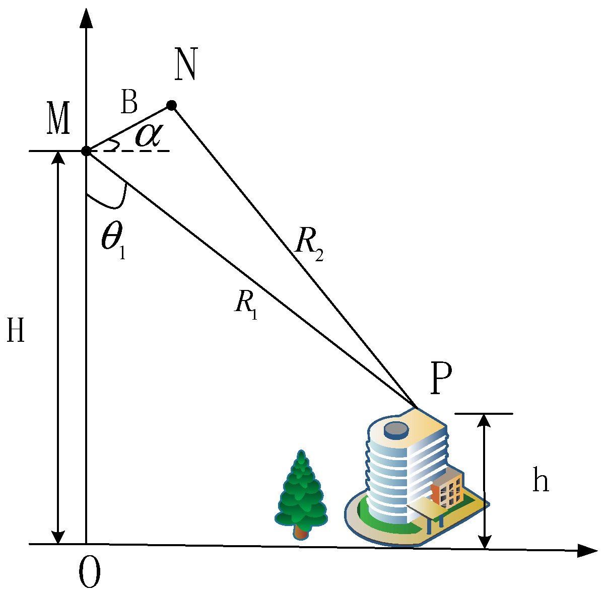
2.1.1. Interferometric SAR Model

InSAR can be used in height inversion through obtaining phase difference between two antennas. The schematic diagram of InSAR is shown in Figure 1, in which H means platform height, M and N represent two antennas, ${\theta }_1$ is incidence angle, B means length of baseline, $\alpha$ is baseline angle. $R_1$ and $R_2$ are the range between antenna and targets and h represents the target’s height.

Two complex images after registration can be expressed as $s_1$, $s_2$ and the interferometric phase can be obtained according to the following equation:

$${\varphi }_w=\arg (s_1{s}_2^{*})$$

(1)

where “arg” means calculating phase, ${\varphi }_{\omega }$ is a wrapping phase whose value is between $-\pi$ and $\pi$. The unwrapping phase $\varphi$ can be obtained through phase unwrapping and it can be expressed as follows:

$$\varphi =-\frac{2\pi Q}{\lambda }(R_1-R_2)$$

(2)

If one antenna transmits signal and two antennas receive, then Q = 1. If the two antennas transmit and receive, respectively, then Q = 2. According to the geometrical relationship in Figure 1, we can obtain the following:

$$\sin \left({\theta }_1-\alpha \right)=\frac{R_1^2-R_2^2+B^2}{2R_{1}B}$$

(3)

Bringing Equation (2) into Equation (3), we can obtain a relationship between incidence angle and unwrapping phase.

$${\theta }_1=\alpha +\arcsin \left(\frac{B}{2R_1}-\frac{\lambda \varphi }{2\pi QB}-\frac{{\lambda }^2{\varphi }^2}{8{\pi }^2{Q}^2{R}_{1}B}\right)$$

(4)

Based on the geometrical relationship between platform and target, we can retrieve target height as follows:

$$h=H-R_1\cos {\theta }_1$$

(5)

Respectively, the sensitivity of height to interferometric phase, baseline, and baseline angle is shown as follows:

$$\begin{gathered} \frac{\partial h}{\partial \varphi }=\frac{\lambda R_1\sin {\theta }_1}{2\pi QB\cos \left({\theta }_1-\alpha \right)} \\ \frac{\partial h}{\partial B}=\frac{\lambda \varphi R_1\sin {\theta }_1}{2\pi Q{B}^2\cos \left({\theta }_1-\alpha \right)} \\ \frac{\partial h}{\partial \alpha }=R_1\sin {\theta }_1 \end{gathered}$$

(6)

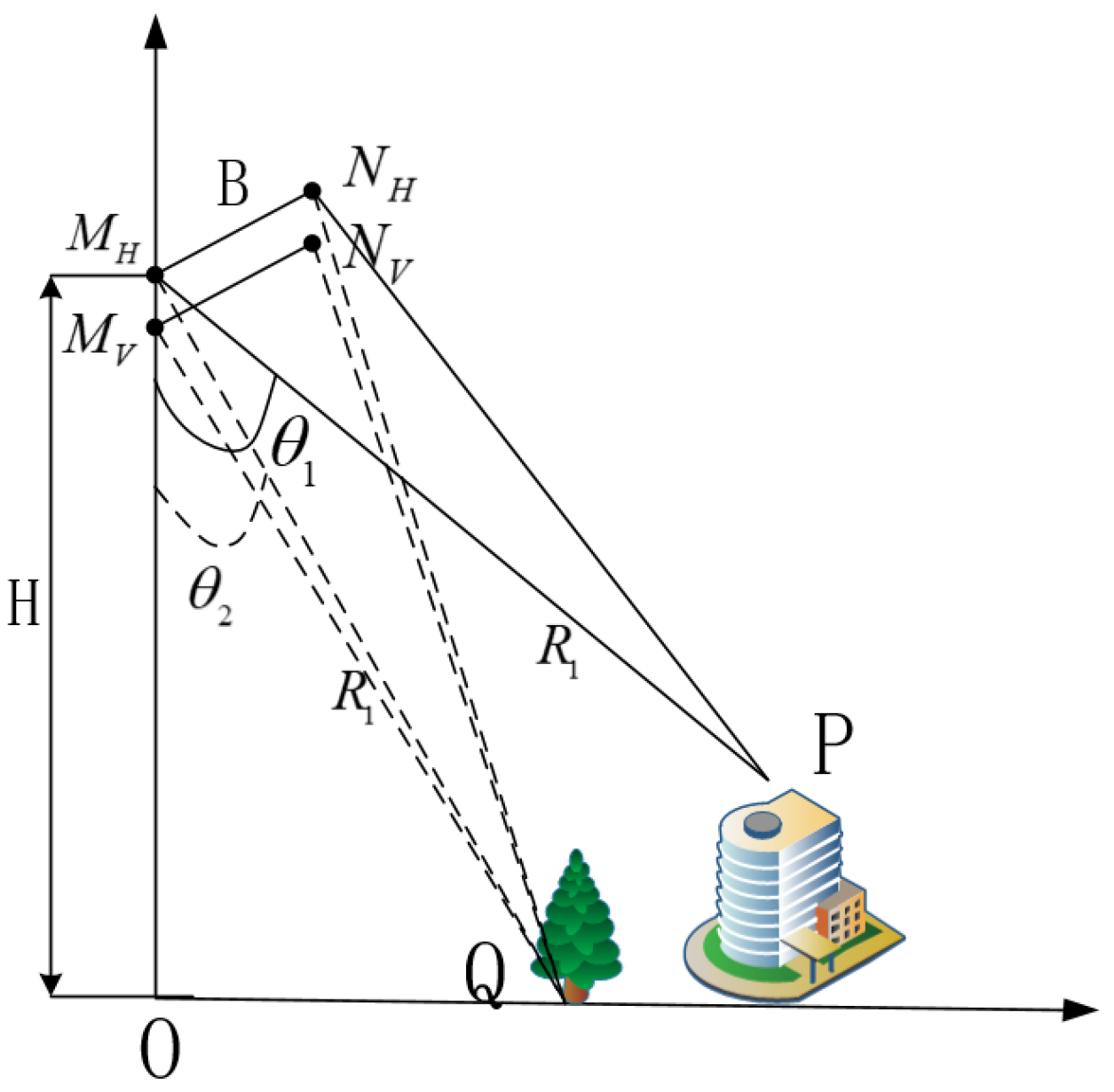
2.1.2. PolInSAR Optimal Coherence Model

PolInSAR can improve coherence compared with InSAR through combining four polarization modes. PolInSAR can obtain two groups of full polarized images. Each pixel in a full polarized image has a corresponding scattering matrix S, where S is a 2 × 2 complex matrix. Therefore, two polarized scattering matrices for the same pixel can be obtained, named as ${\mathit{S}}_{\mathbf{1}}$, ${\mathit{S}}_{\mathbf{2}}$.

$$\begin{array}{l}{\mathit{S}}_{\mathbf{1}}=\left[\begin{array}{cc}{S}_{HH}^1& S_{HV}^1\\ S_{VH}^1& S_{VV}^1\end{array}\right]\\ {\mathit{S}}_{\mathbf{2}}=\left[\begin{array}{cc}{S}_{HH}^2& S_{HV}^2\\ S_{VH}^2& S_{VV}^2\end{array}\right]\end{array}$$

(7)

where H represents horizontal polarization, V represents vertical polarization. The subscript HV means that V transmits and H receives the signal.

The scattering matrix S can also be written in a vector to obtain the polarization vector k based on Pauli decomposition.

$$\begin{array}{l}{\mathit{k}}_{\mathbf{1}}=\frac{1}{\sqrt{2}}{\left[S_{HH}^1+S_{VV}^1,S_{HH}^1-S_{VV}^1,2S_{HV}^1\right]}^T\\ {\mathit{k}}_{\mathbf{2}}=\frac{1}{\sqrt{2}}{\left[S_{HH}^2+S_{VV}^2,S_{HH}^2-S_{VV}^2,2S_{HV}^2\right]}^T\end{array}$$

(8)

where k is a 3 × 1 complex vector.

Next, the following variables are defined:

$$\begin{array}{l}\left[T_{11}\right]=<{\mathit{k}}_{\mathbf{1}}\cdot {\mathit{k}}_{\mathbf{1}}^{+}>\\ \left[{\mathrm{\Omega }}_{12}\right]=<{\mathit{k}}_{\mathbf{1}}\cdot {\mathit{k}}_{\mathbf{2}}^{+}>\\ \left[{\mathrm{\Omega }}_{21}\right]=<{\mathit{k}}_{\mathbf{2}}\cdot {\mathit{k}}_{\mathbf{1}}^{+}>\\ \left[T_{22}\right]=<{\mathit{k}}_{\mathbf{2}}\cdot {\mathit{k}}_{\mathbf{2}}^{+}>\end{array}$$

(9)

where ‘+’ is conjugate transpose and ‘< >’ is average.

In order to improve the coherence of ${\mathit{k}}_{\mathbf{1}}$ and ${\mathit{k}}_{\mathbf{2}}$, the following projection is made:

$$\begin{array}{l}{i}_1={\mathit{w}}_{\mathbf{1}}^{+}{\mathit{k}}_{\mathbf{1}}\\ i_2={\mathit{w}}_{\mathbf{2}}^{+}{\mathit{k}}_{\mathbf{2}}\end{array}$$

(10)

where ${\mathit{w}}_{\mathbf{1}}$, ${\mathit{w}}_{\mathbf{2}}$ are 3 × 1 complex unit vectors. Then we need to find a group of ${\mathit{w}}_{\mathbf{1}}$ and ${\mathit{w}}_{\mathbf{2}}$ to maximize the coherence of $i_1$ and $i_2$. The coherence is as follows:

$$r=\frac{<i_1\cdot i_2^{+}>}{\sqrt{<i_1\cdot i_1^{+}><i_2\cdot i_2^{+}>}}=\frac{<{\mathit{w}}_{\mathbf{1}}^{+}\left[{\Omega }_{12}\right]{\mathit{w}}_{\mathbf{2}}>}{\sqrt{<{\mathit{w}}_{\mathbf{1}}^{+}\left[T_{11}\right]{\mathit{w}}_{\mathbf{1}}><{\mathit{w}}_{\mathbf{2}}^{+}\left[T_{22}\right]{\mathit{w}}_{\mathbf{2}}>}}$$

(11)

According to the PolInSAR optimal coherence method [2], we have the following:

$$\begin{array}{l}{\left[T_{11}\right]}^{-1}\left[{\mathrm{\Omega }}_{12}\right]{\left[T_{22}\right]}^{-1}{\left[{\mathrm{\Omega }}_{12}\right]}^{+}{\mathit{w}}_{\mathbf{1}}={\lambda }_1{\lambda }_2^{+}{\mathit{w}}_{\mathbf{1}}\\ {\left[T_{22}\right]}^{-1}{\left[{\mathrm{\Omega }}_{12}\right]}^{+}{\left[T_{11}\right]}^{-1}\left[{\mathrm{\Omega }}_{12}\right]{\mathit{w}}_{\mathbf{2}}={\lambda }_1{\lambda }_2^{+}{\mathit{w}}_{\mathbf{2}}\end{array}$$

(12)

where ${\lambda }_1$, ${\lambda }_2$ are coefficients of Lagrange and $v={\lambda }_1{\lambda }_2^{+}$ is defined as an eigenvalue. Afterward, we obtain three real eigenvalues $v_1$, $v_2$, $v_3$, and three pairs of eigenvectors that are $\left\{{\mathit{w}}_{\mathbf{1}},{\mathit{w}}_{\mathbf{2}}\right\}$, $\left\{{\mathit{w}}_{\mathbf{3}},{\mathit{w}}_{\mathbf{4}}\right\}$, $\left\{{\mathit{w}}_{\mathbf{5}},{\mathit{w}}_{\mathbf{6}}\right\}$.

To ensure that all interferometric phase information is contained in $k_1·k_2^{+}$, the following equation should be satisfied.

$$\arg \left({\mathit{w}}_i^{+}{\mathit{w}}_{i+1}\right)=0\begin{array}{cc}& \left(i=1,3,5\right)\end{array}$$

(13)

where “arg” means calculating phase.

There are several ways to satisfy the condition in Equation (13). According to [30], we use the following:

$$\begin{array}{c}{\mathit{\omega }}_i={\mathit{w}}_i\exp \left(-j{\varphi }_e/2\right)\\ {\mathit{\omega }}_{i+1}={\mathit{w}}_{i+1}\exp \left(j{\varphi }_e/2\right)\end{array}$$

(14)

where ${\varphi }_e=\arg \left({\mathit{w}}_i^{+}{\mathit{w}}_{i+1}\right)$.

Then, we can choose the maximum eigenvalue $v_1$ and its corresponding eigenvectors $\left\{{\mathit{\omega }}_{\mathbf{1}},{\mathit{\omega }}_{\mathbf{2}}\right\}$ to generate polarimetric interferometry fringes.

$${\varphi }_{opt}=\arg \left(i_1{i}_2^{+}\right)$$

(15)

where

$$\begin{array}{l}{i}_1={\mathit{\omega }}_{\mathbf{1}}^{+}{\mathit{k}}_{\mathbf{1}}\hfill \\ i_2={\mathit{\omega }}_{\mathbf{2}}^{+}{\mathit{k}}_{\mathbf{2}}\hfill \end{array}$$

(16)

Here $i_1$ and $i_2$ are the projections of $k_1$ and $k_2$ from the polarized Pauli basis space into the one-dimensional space. Through the polarimetric interferometric optimal decomposition, we can improve coherence and obtain the interferometric phase ${\varphi }_{opt}$ under optimal coherence. However, meaning of interferometric phase is not clear. Besides, we also do not know the relationship among ${\varphi }_{opt}$ and other interferometric phases of different scattering mechanisms in the same pixel.

Therefore, we propose a procedure to show their relationship.

The polarization vector k can be expressed as follows:

$$\begin{array}{l}{\mathit{k}}_{\mathbf{1}}={\left[k_{11},k_{12},k_{13}\right]}^T\\ {\mathit{k}}_{\mathbf{2}}={\left[k_{21},k_{22},k_{23}\right]}^T\end{array}$$

(17)

where $k_{11}$, $k_{12}$, $k_{13}$ are respectively represent three Pauli decompositions that are single scattering, double scattering of 0 degrees, and double scattering of 45 degrees, denoted as $P_s$, $P_d$ and $P_v$_, respectively.

The two groups of projection directions are as follows:

$$\begin{array}{l}{\mathit{\omega }}_{\mathbf{1}}={\left[{\omega }_{11},{\omega }_{12},{\omega }_{13}\right]}^T\\ {\mathit{\omega }}_{\mathbf{2}}={\left[{\omega }_{21},{\omega }_{22},{\omega }_{23}\right]}^T\end{array}$$

(18)

According to our derivation, we can obtain the following equations and the corresponding derivation is listed in Appendix A:

$$\begin{array}{l}\sin {\varphi }_{opt}=\\ \frac{\left|{\omega }_{11}\right|\left|k_{11}\right|}{\left|i_1\right|}\sin [{\varphi }_{m_1}+({\varphi }_{k_{21}}-{\varphi }_{w_{11}}-{\varphi }_{i_2})]\\ +\frac{\left|{\omega }_{12}\right|\left|k_{12}\right|}{\left|i_1\right|}\sin [{\varphi }_{m_2}+({\varphi }_{k_{22}}-{\varphi }_{w_{12}}-{\varphi }_{i_2})]\\ +\frac{\left|{\omega }_{13}\right|\left|k_{13}\right|}{\left|i_1\right|}\sin [{\varphi }_{m_3}+({\varphi }_{k_{23}}-{\varphi }_{w_{13}}-{\varphi }_{i_2})]\end{array}$$

(19)

where $m_{opt}=i_1{i}_2^{+}$, $m_1=k_{11}{k}_{21}^{+}$, $m_2=k_{12}{k}_{22}^{+}$, $m_3=k_{13}{k}_{23}^{+}$. ${\varphi }_{m1}$, ${\varphi }_{m2}$, ${\varphi }_{m3}$ are, respectively, the interferometric phases of Pauli decomposition, ${\varnothing }_{opt}$ is the interferometric phase of polarimetric interferometric optimal decomposition.

In Section 3, we will continue to analyze the relationship using simulation and real data.

2.1.3. Height Difference

To analyze the scattering mechanism of the targets in PolInSAR, the absolute height error has little effect, but the relative height error has an important impact. Therefore, it is necessary to analyze the influence of the system parameters on the height difference between different polarization modes.

Supposing there are two targets within the same pixel, as P and Q in Figure 2. They have different heights and different scattering mechanisms, and they have the same slant range $R_1$ as they are in the same pixel. In Figure 2, $M_H$, $M_V$, $N_H$, and $N_V$ are antennas, where $M_H$ and $N_H$ represent antenna H. $M_V$ and $N_V$ represent antenna V. ${\theta }_1$ and ${\theta }_2$ are, respectively, the incidence angles of P and Q.

The height difference can be expressed as Equation (20) according to Equation (5).

$$\Delta h=h_1-h_2=-R_1\left(\sin {\theta }_1-\sin {\theta }_2\right)$$

(20)

The sensitivity of height difference to baseline length, baseline angle, and interferometric phase can be calculated as follows:

$$\frac{\partial \Delta h}{\partial B}=\frac{\lambda R_1}{2\pi Q{B}^2}\left(\frac{{\varphi }_1\sin {\theta }_1}{\cos \left({\theta }_1-\alpha \right)}-\frac{{\varphi }_2\sin {\theta }_2}{\cos \left({\theta }_2-\alpha \right)}\right)$$

(21)

$$\frac{\partial \Delta h}{\partial \alpha }=R_1\left(\sin {\theta }_1-\sin {\theta }_2\right)$$

(22)

$$\frac{\partial \Delta h}{\partial \varphi }=\frac{\lambda R_1\sin {\theta }_1}{2\pi QB\cos \left({\theta }_1-\alpha \right)}-\frac{\lambda R_1\sin {\theta }_2}{2\pi QB\cos \left({\theta }_2-\alpha \right)}$$

(23)

According to the above equations, we can analyze the height difference error caused by system error. Here, we use the parameters of this PolInSAR system shown in

Table 1. Parameters of The PolInSAR System.

Parameters	Value
Frequency	15.2 GHz
Baseline	0.62 m
Bandwidth	1.2 GHz
Platform Height	206 m
Incidence Angle	70°
Resolution	0.3 m

. We can obtain the sensitivity of height difference to baseline is $4\times {10}^{-4}$, sensitivity of height difference to baseline angle is $-2\times {10}^{-5}$ m/rad, and sensitivity of height difference to interferometric phase is $-9\times {10}^{-10}$ m/$°$, which means even if the baseline error is 1 m, the baseline angle error is 10 rad, and the interferometric phase error is ${10}^6$ degrees, the height difference error is only in ${10}^{-4}$ m. Therefore, baseline, baseline angle, and interferometric phase errors have little influence on the height difference between two polarization modes. So, we have reasons to believe that the height difference extracted from this PolInSAR data reflects the difference in the target-scattering mechanism.

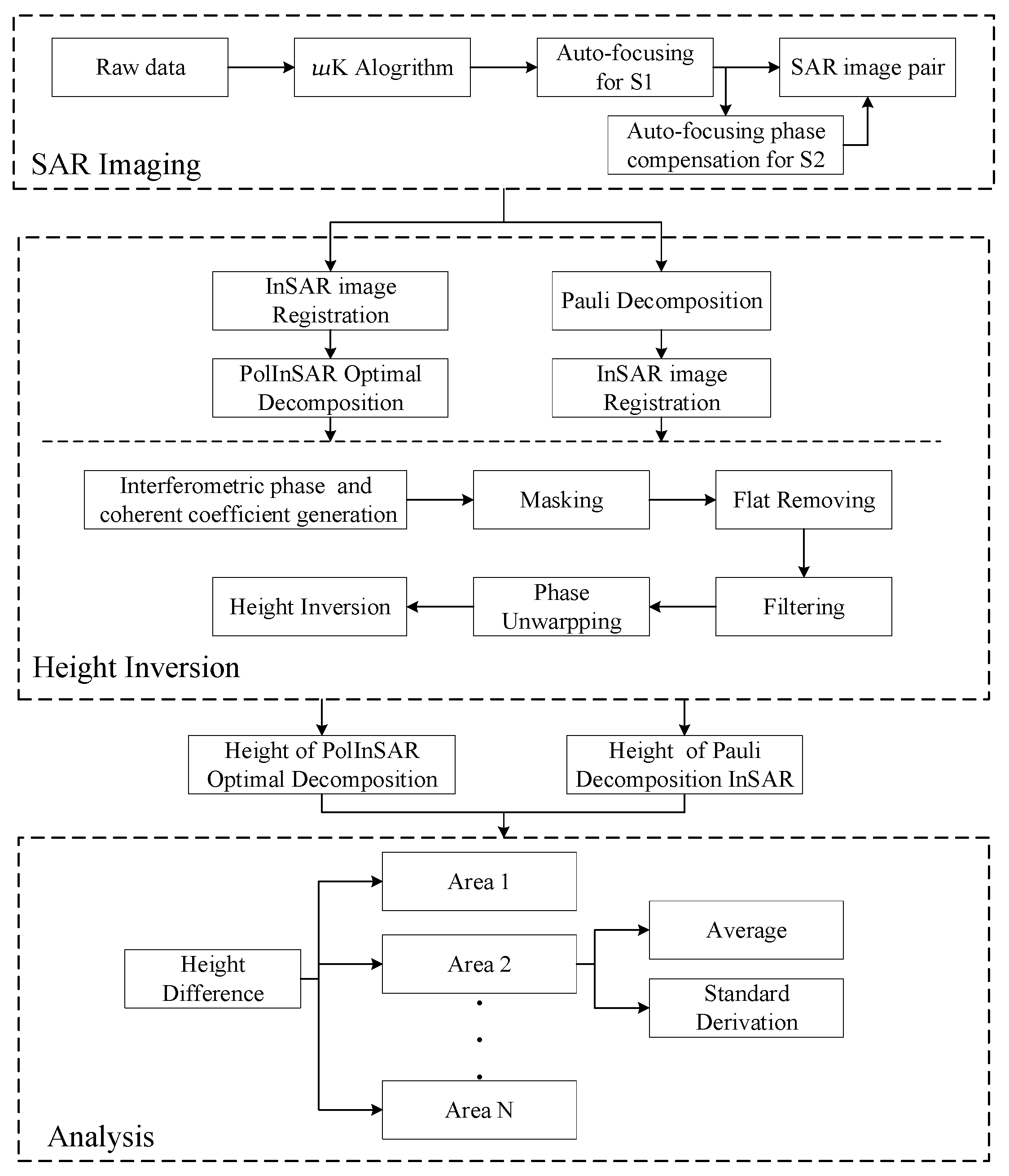
2.2. Data Processing Methodology

The flow chart of the process to retrieve targets’ heights is shown in Figure 3. The process is divided into the following three parts: SAR imaging, height inversion, and analysis.

In SAR imaging, we use $\omega -k$ algorithm and PGA auto-focusing algorithm to obtain SAR images. In height inversion, the height of targets can be obtained through processing of InSAR of different modes. In analysis, the height difference of different polarization modes is compared and analyzed combined with optical images.

2.2.1. Imaging

We apply $\omega -k$ algorithm with one-step motion compensation and self-autofocusing algorithm to obtain well-focused SAR images. The $\omega -k$ algorithm is a common algorithm for high-resolution SAR imaging. When the platform velocity is constant, the algorithm can correct range migration over a wide range of apertures or large oblique viewing angles. However, for UAV-borne SAR, the motion trajectory is often an irregular curve due to airflow disturbance and other effects, which can lead to energy dispersion and severe degradation of imaging quality. So, one-step motion compensation method [31] is applied to obtain high precision in motion compensation.

During the imaging process, we compensate for the motion error according to the center of the radar beam, which leads to a residual motion compensation error in the azimuthal direction. In our previous work [17], we analyzed the influence of RMCE on this UAV-borne PolInSAR system using the same data. When there is a 20-m height difference between the target and the reference height while imaging, the residual polarimetric interferometric phase is about 12 degrees, which will cause an absolute height error of 2 m. As we mentioned before, even if there is an absolute height deviation, it does not affect the height difference between different scatters with different polarization scattering, so this is acceptable.

However, the residual motion error after motion compensation will still cause defocusing; therefore, we use the phase gradient autofocus (PGA) algorithm [32] to estimate and compensate for the residual error. To ensure that PGA will not introduce new phase errors between InSAR image pairs, we perform PGA for the transmitter and obtain the estimated phase error, and then compensate the receiver data with the same phase error.

After obtaining SAR images, two groups of full-polarimetric images of the same area are registered, and then the data is processed according to the following steps.

2.2.2. Pauli Decomposition and Optimal Coherence Decomposition

Based on the focused PolSAR images, we perform Pauli decomposition to decompose the scattering matrix S into the weighted sum of the complex numbers of each Pauli matrix, which means we obtain ${\mathit{k}}_{\mathbf{1}}$,${\mathit{k}}_{\mathbf{2}}$ in Equation (8). Then we perform calculations according to Equations (7)–(16) to obtain $i_1$,$i_2$ for further process.

2.2.3. Height Inversion

• Interferometric Phase and Coherent Coefficient Generation

We calculate the interferometric phase of each component of ${\mathit{k}}_{\mathbf{1}}$ and ${\mathit{k}}_{\mathbf{2}}$, and also the interferometric phase of $i_1$ and $i_2$. Meanwhile, we calculate the coherent coefficient of $k_1$ and $k_2$, and of $i_1$ and $i_2$ for further processing.

2.

Masking

For InSAR, small coherence coefficient will cause a significant error in the results. Therefore, the pixels with higher coherence are firstly selected. Here we chose those pixels whose coherence coefficients are better than 0.8, and the coherence window is $5\times 5$. However, we discover that the extracted pixels are fragments, so the method of expansion and corrosion is used to obtain a better mask. We use corrosion first, whose window is $3\times 3$, and expansion next, whose window is $5\times 5$. The following processing and analysis are all carried out for these exacted pixels.

3.

Flat Removing and Filtering

The “flat-earth effect” of InSAR makes the interferometric fringes too dense, so we remove the flat-earth effect before the phase unwrapping. Then, we use the classical method of frequency filtering called Goldstein filtering [33,34] to obtain filtered phase map, where the power exponent of the frequency domain function α is 0.5 and the filtering window is $16\times 16$.

4.

Phase Unwrapping

Phase unwrapping is used to remove the period in phase, but in urban areas it is very difficult. However, when specific conditions are met, we do not need to perform phase unwrapping.

According to the sensitivity of height to interferometric phase in Equation (6), $\frac{\partial h}{\partial \varphi }$ here is about 8.4 rad/m. So, the unambiguous height is 52.8 m, which is to say height changes about 52.8 m when the interferometric phase changes ${360}^{°}$. The maximum targets’ height in our selected area is about 35 m that is lower than height unambiguity of InSAR. Therefore, we do not need to perform phase unwrapping here.

5.

Height Inversion

We retrieve targets’ height according to Equation (5). The height maps are denoted as $P_1,P_2,P_3$, and $I_1$, which are inversed by the components of ${\mathit{k}}_{\mathbf{1}}$,${\mathit{k}}_{\mathbf{2}}$ and by $i_1,i_2$, respectively. The height is set to zero for those pixels that are not selected by the mask.

2.2.4. Height Difference Analysis

To explore the application and the height inversion results of PolInSAR, we choose typical area of different targets in the image and make comparison of $P_1,P_2,P_3$ and $I_1$, including calculating height difference, the mean value of the height difference, and the standard deviation of the height difference. Then, the results are analyzed through simulation. $P_1,P_2,P_3$ means height inversion results from three Pauli decompositions and $I_1$ means height inversion results from polarimetric interferometric optimal decomposition.

3. Results

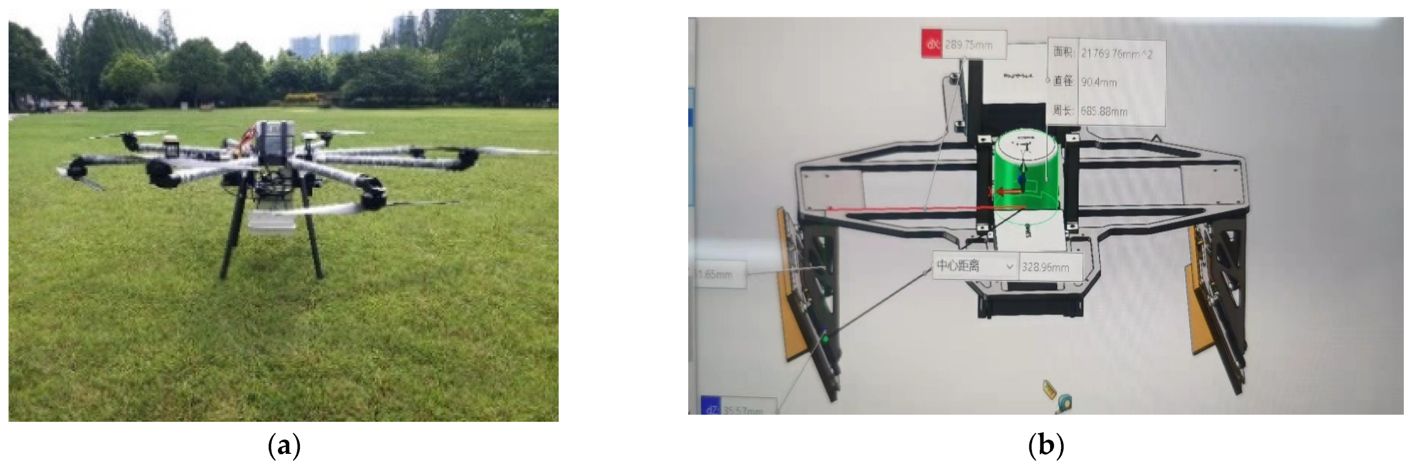
3.1. System and Experimental Data

The PolInSAR data we processed and studied was acquired by a small UAV-borne Ku-band PolInSAR system jointly developed by ZhongKeYuDa company and AIRCAS in 2020. The system parameters are listed in Table 1; the system is shown in Figure 4.

Figure 4a is the photo of the system, and Figure 4b shows the inner structure of the system. In Figure 4b, the green cylinder in the middle is the POS (Position and Orientation System), and the antennas are on both sides. The distance between POS and one antenna in a horizontal direction $dx$ is 289.75 mm. The distance between POS and one antenna is 328.96 mm. The area of the POS is $21,769.76 {\mathrm{mm}}^2$, the diameter is 90.4 mm, and the perimeter is 685.88 mm.

The imaging area is shown in Figure 5. It is located at Fudan University, Shanghai, China with a campus, several teaching buildings, many residential buildings, and trees.

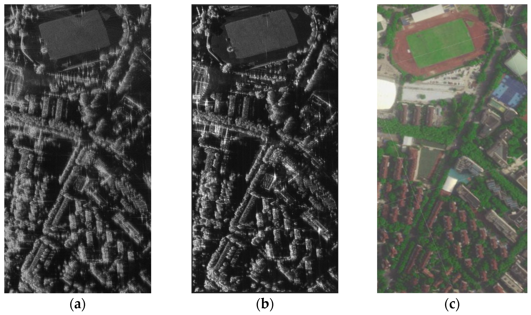
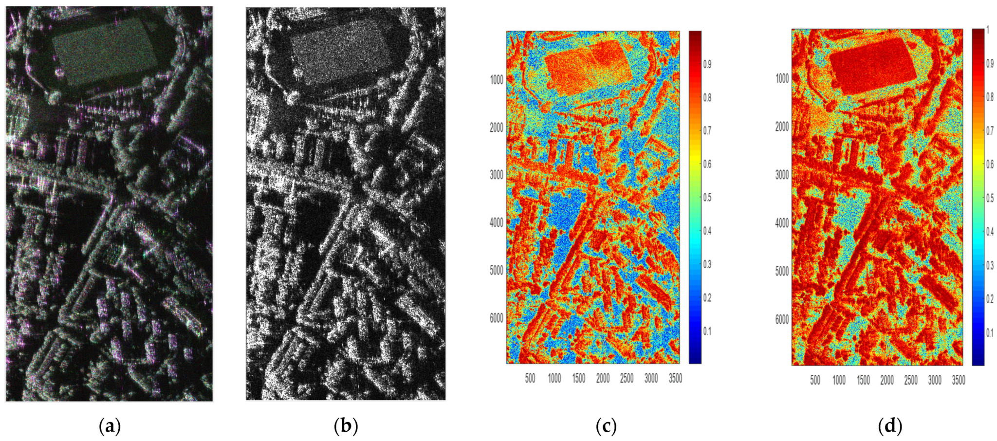
3.2. Pauli Decomposition and Optimal Coherence Decomposition Results

The pseudo color image of Pauli decomposition is shown in Figure 6a, the image of $i_1$ is shown in Figure 6b, and the coherence between $k_{11}$ and $k_{21}$ is shown in Figure 6c, and the coherence between $i_1$ and $i_2$ is shown in Figure 6d. It shows that the coherence is greatly improved after the optimal polarization coherence processing. The coherence is higher than 0.9 for those buildings and trees that are not in shadows, which is quite good for further processing.

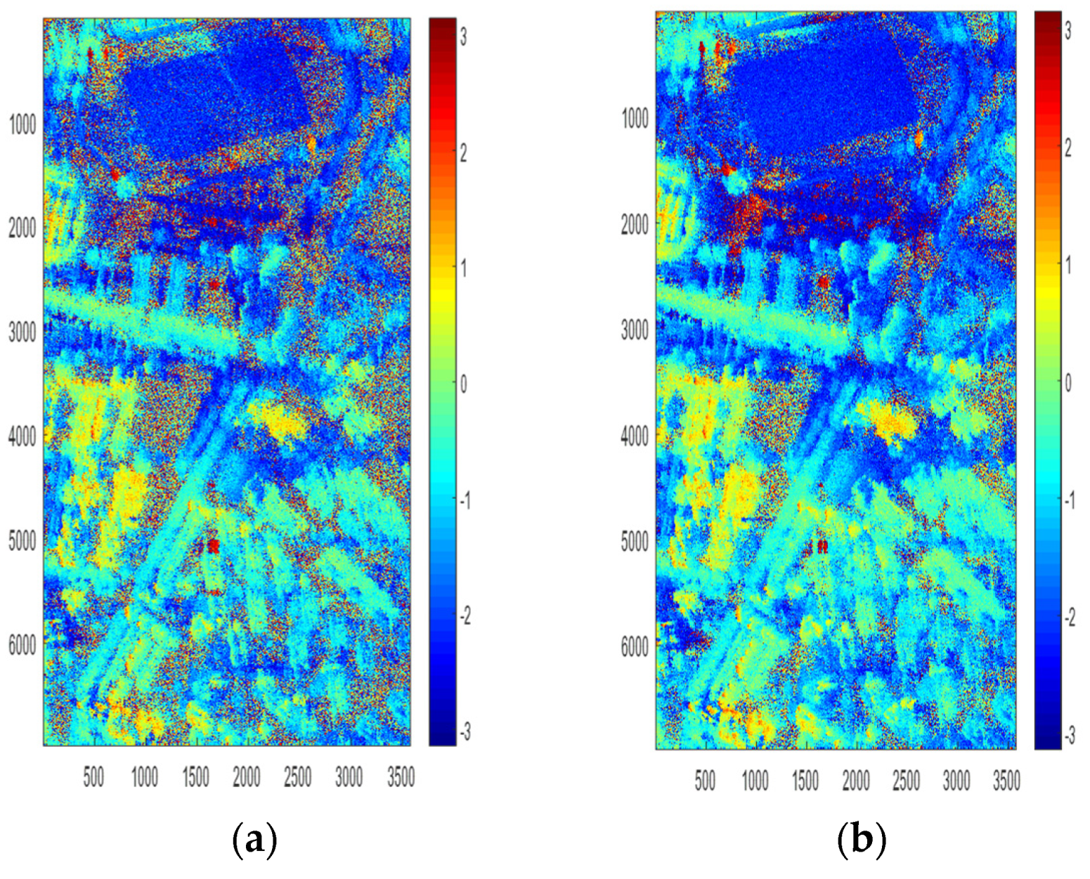
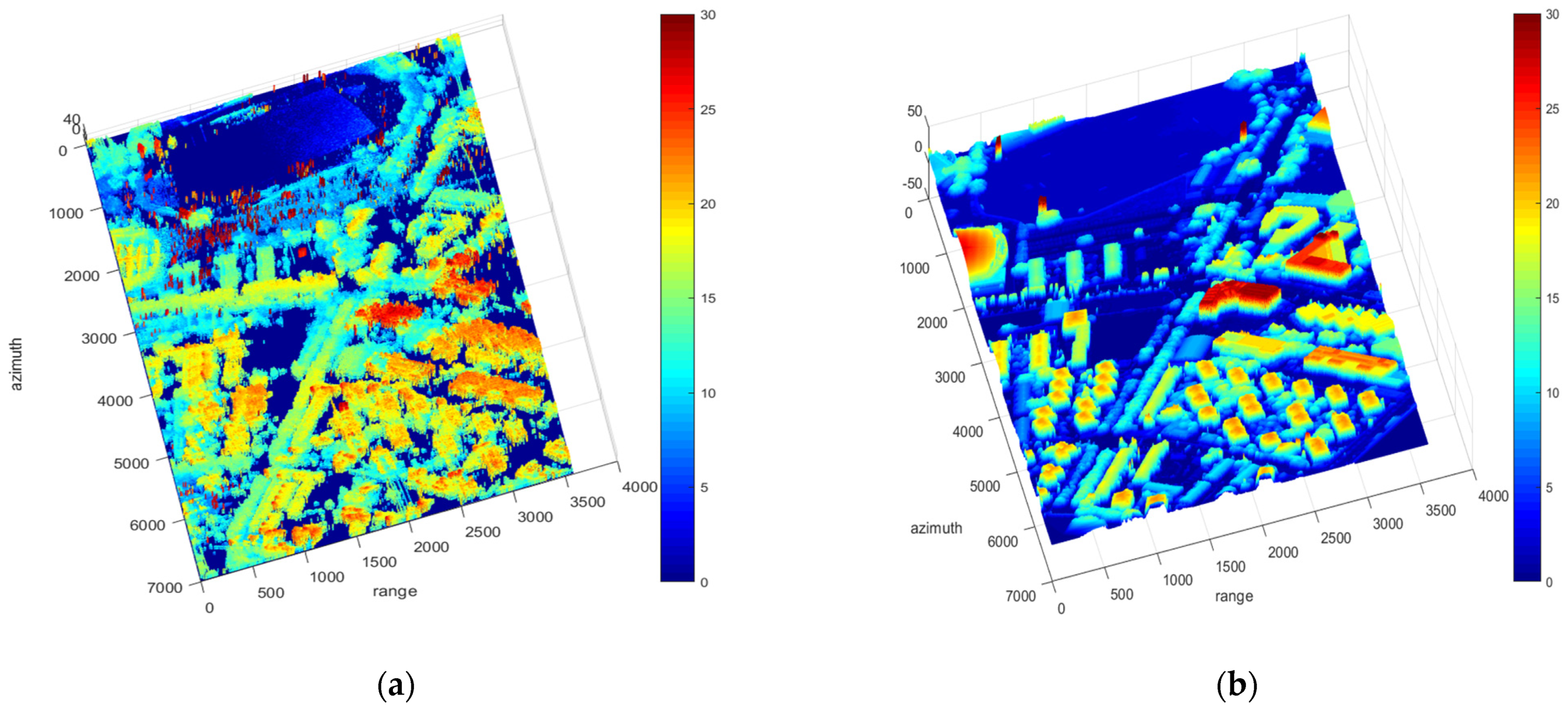
3.3. Interferometric Phase and Height Inversion Results

The interferometric phase after flat-removing and phase filtering of $k_{11}$, $k_{21}$, and $i_1$, $i_2$ is shown in Figure 7.

The height inversion results with a mask are shown in Figure 8 and Figure 9a.

The real height obtained by optical oblique photography is shown in Figure 9b. It can be seen that the heights of the buildings and trees are obtained. In building areas, the mean error of PolInSAR is −0.57 m, the standard deviation of error is 2.83 m, and the RMSE is 2.88 m. It shows that our error in DSM is acceptable. Besides, the RMSE of $P_s$, $P_d$ and $P_v$ are, respectively, 3.16 m, 3.21 m, and 3.39 m. It shows that the height obtained by PolInSAR is more accurate than that by Pauli decomposition.

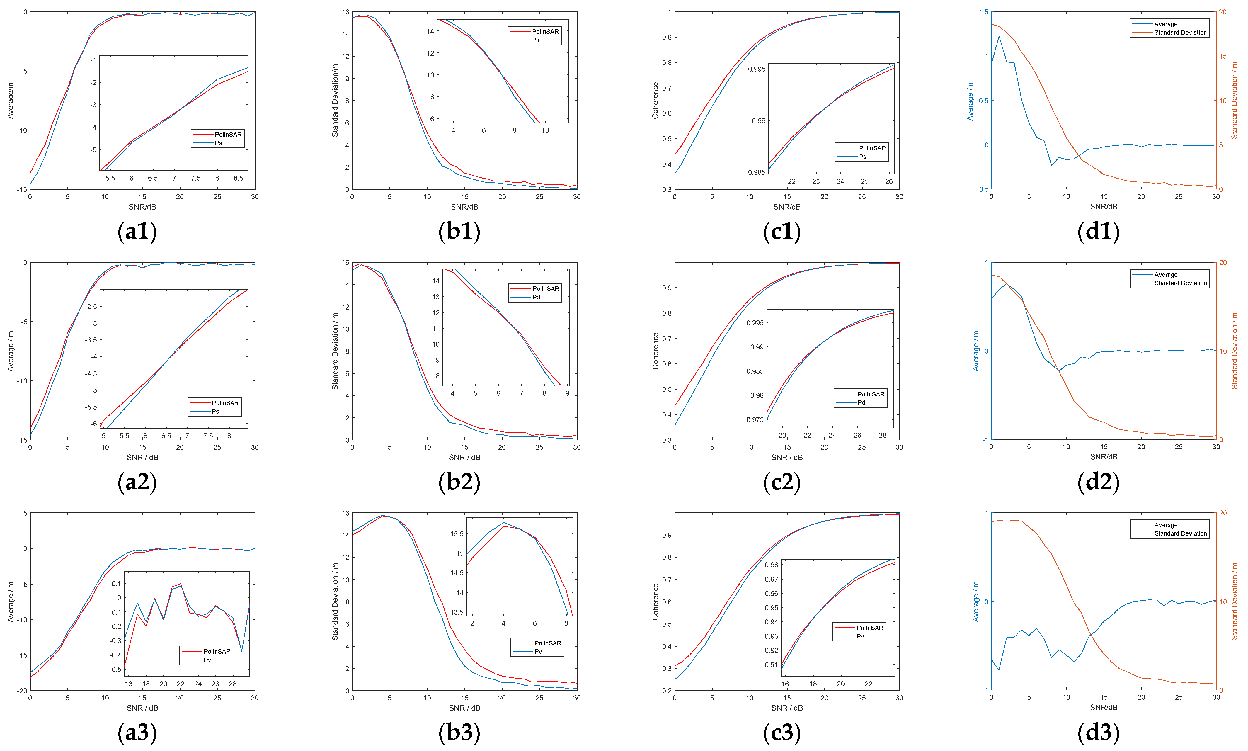
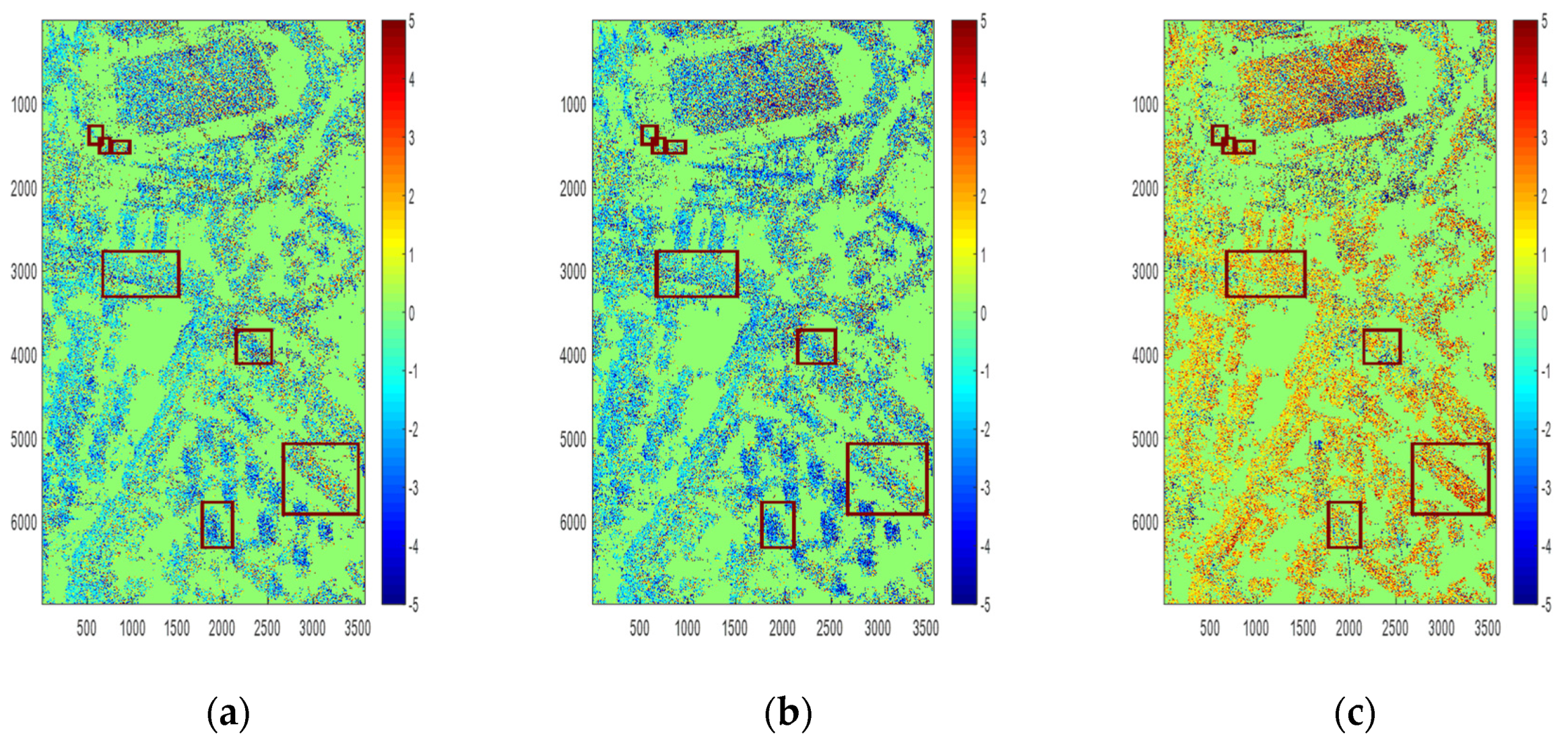
3.4. Height Inversion Results of Typical Targets

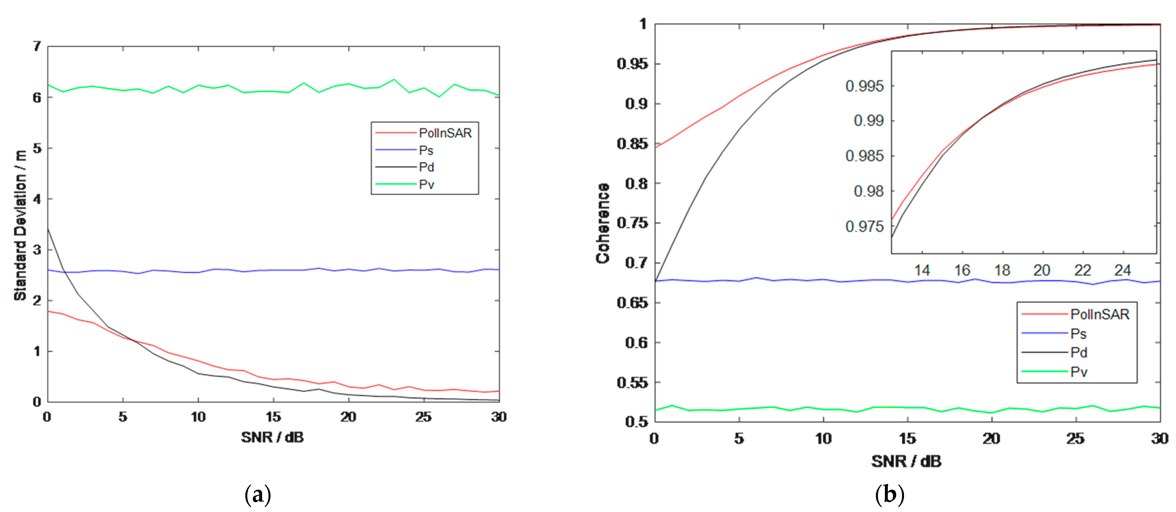
To explore the PolInSAR results in urban areas, we chose some typical targets in the observation area and made comparisons of the heights retrieved by different polarimetric components. The selected targets are shown in Figure 10.

These areas contain artificial targets and trees. Area 1 is a lamppost in a stadium whose height is about 30 m. Areas 2 and 3 are both teaching buildings whose roofs are uneven. Area 4 is a residential building whose roof is sloping. Areas 5 to 7 are all sycamore trees but with different heights, where trees in area 5 are about 10 m and the others are about 15 m.

The heights of the targets and the height difference between different polarimetric components of these targets are shown in Figure 11. The height retrieved by PolInSAR is shown in Figure A1a, and the height difference between PolInSAR and Pauli decomposition is shown in Figure A1b–d. Figure A1 is shown in Appendix B. Each row represents a selected area. It can be seen from Figure A1 that the height of the lamppost is between 25 and 30 m, which is in line with the actual situation. The heights of the trees range from 10 m to 15 m, which is also reasonable.

Then, the mean values and standard deviations of height differences of these selected areas are listed in

Table 2. Mean value of height difference using UAV data.

Area	Average
	${\mathit{I}}_1-{\mathit{P}}_1$	${\mathit{I}}_1-{\mathit{P}}_2$	${\mathit{I}}_1-{\mathit{P}}_3$	${\mathit{P}}_2-{\mathit{P}}_1$	${\mathit{P}}_3-{\mathit{P}}_1$
1	−0.23	−0.33	1.15	0.10	−1.39
2	−0.85	−1.07	1.02	0.22	−1.87
3	−0.26	−0.69	1.42	0.43	−1.68
4	−1.69	−2.25	1.02	0.56	−2.71
5	−1.13	−1.24	0.94	0.10	−2.07
6	−0.64	−0.87	0.48	0.24	−1.12
7	−0.77	−0.84	1.27	0.07	−2.04

, where $I_1$ represents height retrieved by polarimetric interferometry optimal decomposition. $P_1,P_2,P_3$, respectively, represents height retrieved by single scattering, double scattering of 0 degrees, and double scattering of 45 degrees. The values marked in bold represent the smallest average values of height difference.

It can be seen from Table 2 that, as for the lamppost in Area 1, the height of polarimetric interferometry optimal decomposition is close to the height of single scattering. It can also be seen that the average values of $P_2-P_1$ are quite small while the average values of $P_3-P_1$ are bigger, which means single scattering and double scattering of 0 degrees are closer.

For buildings with uneven roofs in Areas 2 and 3, the height of polarimetric interferometry optimal decomposition is close to the height of single scattering. For the building with a sloping roof in Area 4, the phase center of PolInSAR is close to a double scattering of 45 degrees.

As for the tree areas, the absolute average value of $I_1-P_1$, $I_1-P_2$, $I_1-P_3$ are quite close, which seems no dominant scattering can represent the height of the area.

3.5. Analysis

To analyze the above results and to explore the relationship between Pauli decompositions and optimal coherence decomposition, we perform simulations in this part.

First, a simulated area is generated whose size is 100 ∗ 100. The half part on the left is the ground, whose height is 0 m, and the half part on the right is the target, whose height is 20 m. The height of the simulated area is shown in Figure 12.

The scattering matrix of the target has different cases, and it is expressed as follows:

Case 1: one scattering mechanism in a pixel, where scattering matrix can be as follows:

$$s_g=\left[\begin{array}{cc}1& 0\\ 0& 1\end{array}\right]{\sigma }_g,s_h=\left[\begin{array}{cc}1& 0\\ 0& 1\end{array}\right]{\sigma }_h$$

(24)

$$s_g=\left[\begin{array}{cc}1& 0\\ 0& 1\end{array}\right]{\sigma }_g,s_h=\left[\begin{array}{cc}1& 0\\ 0& -1\end{array}\right]{\sigma }_h$$

(25)

$$s_g=\left[\begin{array}{cc}1& 0\\ 0& 1\end{array}\right]{\sigma }_g,s_h=\left[\begin{array}{cc}0& 1\\ 1& 0\end{array}\right]{\sigma }_h$$

(26)

Case 2: three scattering mechanisms in a pixel with similar or different scattering coefficients.

Here, $s_h$ in Equation (24) is single scattering, in Equation (25) is double scattering of 0 degrees, and in Equation (26) is double scattering of 45 degrees. ${\sigma }_g$ and ${\sigma }_h$ are the backscattering coefficients of the ground and the target, respectively, where ${\sigma }_g$ and ${\sigma }_h$ are different under different SNR conditions.

In the process of polarimetric interferometry, the window is set to be 7 ∗ 7. We can find a boundary phenomenon in the middle of the area. Hence, the boundary is not counted when calculating.

3.5.1. One Scattering Mechanism in a Pixel

We suppose there is only one scatter in a pixel. After giving coefficients of three Pauli decompositions and height, we can obtain the height of PolInSAR and Pauli decomposition according to the processing of InSAR.

The procedure of simulation uses the location of the target and antenna to generate range and obtain phase. Here, we can obtain the phases of HH, HV, VH, and VV. Next, the scattering coefficients can be used as amplitude. Therefore, we can obtain the scattering matrix and use it to retrieve height.

We use one situation as an example to show the simulation results. Supposing the SNR of the ground single scattering signal is 20 dB and the SNR of double bounce scattering of an artificial target is 30 dB, and supposing the ground is 0 m, and the artificial target is 20 m in height, the simulated height is shown in Figure 13. It can be seen that the height of single scattering in Figure 13a and the height of double bounce scattering in Figure 13b is better than the height result in Figure 13d, which means optimal coherence decomposition is not suitable for this situation.

Simulation results of different scatterings under different SNRs are also shown in Figure A2 and in Appendix C. The three rows, respectively, represent single scattering, double scattering of 0 degrees, and double scattering of 45 degrees. In columns (a) to (c), the red line is the result of polarimetric interferometric optimal decomposition, and the blue line is the result of the corresponding scattering mechanism. In column (d), the blue line is the average height, and the red line is the standard deviation of height.

From the results in Figure A2 in Appendix C, it can be seen that polarimetric interferometric optimal decomposition can improve coherence when SNR is lower than 20 dB. However, in the aspect of height inversion error, it is larger than the result of Pauli decomposition when there is only one scattering mechanism in a pixel, and it becomes better when SNR is lower than about 6 dB.

3.5.2. Mixed-Scattering Mechanisms in a Pixel

Furthermore, we consider a more common situation of three scattering mechanisms in a pixel. The power of three scatters is set to be the same in this subsection. The simulated results of three different cases while SNR is 30 dB are listed in

Table 3. Simulated height of mixed mechanisms.

Case	Mode	Preset Height (m)	Simulated Height (m)
2.1	$I_1$		9.43
	$P_1$	6	5.86
	$P_2$	12	11.85
	$P_3$	15	14.85
2.2	$I_1$		9.54
	$P_1$	12	11.85
	$P_2$	6	5.85
	$P_3$	15	14.84
2.3	$I_1$		10.64
	$P_1$	6	5.93
	$P_2$	15	14.92
	$P_3$	12	11.93

.

The preset height is the height of the three Pauli decompositions we set before the simulation. The simulated height is the height obtained by simulation.

It shows that the height of polarimetric interferometric optimal decomposition is close to the height of the scattering mechanism at a medium height. Besides, the results under different SNR of Case 2.3 are shown in Figure 14, where Figure 14a is the deviation of simulated height and (b) is coherence. The red line is PolInSAR; the blue, black, and green lines, respectively, represent three Pauli decompositions.

It can be seen that the height obtained by optimal coherence decomposition is more stable when SNR is lower than 10 dB. In Figure 14b, it shows that polarimetric interferometric optimal decomposition can improve coherence when the SNR of images is lower than 22 dB. When the SNR of images is larger than 22 dB, there is no need to perform polarimetric interferometric decomposition because the effect of Pauli decomposition is better.

3.5.3. Mixed-Scattering Mechanism with A Main Scattering Mechanism in a Pixel

In this part, we consider a situation of three mechanisms in a pixel, and the power of one mechanism is larger than the others, which we call the main mechanism in the pixel. The simulated results are shown in Figure 15.

It shows that the height obtained by PolInSAR is more stable when the SNR of the main mechanism is lower than 5 dB and that PolInSAR has a greater coherence when the SNR of the main mechanism is lower than 18 dB.

From the above results for different cases, we find that polarimetric interferometric decomposition can obtain better coherence and height estimation results in the case of a single- or mixed-scattering mechanism when SNR is lower than about 5 dB. When SNR is between 5 dB and 18 dB, better coherence can be obtained by polarimetric interferometric decomposition, but the height results may not be good. When SNR is better than 18 dB, polarimetric decomposition is a better choice than polarimetric interferometric decomposition.

3.5.4. Verification

In Section 2.1.2, we have obtained a relationship of phase center height between polarimetric interferometric optimal decomposition and Pauli decomposition. In Section 3.4, we obtain the experimental results. Here we verify the derivation and the experimental results through simulations.

We calculate the ratio of the amplitude of Pauli decomposition as follows:

$${\xi }_i=\frac{\left|{\displaystyle \sum _{k=1}^{L1\ast L2}{A}_i(k)}\right|}{\left|{\displaystyle \sum _{k=1}^{L1\ast L2}{A}_1(k)}\right|}$$

(27)

where ${\xi }_i$ means amplitude ratio of $i$-th component of Pauli decomposition. A means the amplitude of each pixel.

Then, the amplitude and height of Pauli decomposition are given in our simulation. Then we perform simulations similar to what we perform in Section 3.5.2 and obtain the simulated results called ‘Height result of simulation’. Moreover, we obtain the height results from Equation (19) called ‘Height result of derivation’. The results are shown in

Table 4. Three kinds of height of selected areas.

Case	Mode	Amplitude Ratio	Experimental Height (m)	Height Result of Simulation (m)	Height Result of Derivation (m)
1	$I_1$		25.44	25.89	24.96
	$P_1$	1.00	26.20	25.96	26.15
	$P_2$	0.77	26.80	26.56	26.27
	$P_3$	1.20	23.83	23.59	23.80
2	$I_1$		22.19	22.85	22.69
	$P_1$	1.00	23.07	22.96	23.89
	$P_2$	0.75	23.98	23.88	23.89
	$P_3$	1.88	20.98	20.88	21.17
3	$I_1$		18.25	18.90	18.75
	$P_1$	1.00	18.48	18.44	19.64
	$P_2$	0.87	19.34	19.30	19.65
	$P_3$	0.74	17.66	17.62	17.64

. ‘Experimental Height’ is obtained using UAV data.

It can be seen that the results of the three columns on the right are consistent with each other, which verifies the derivation and the processing of the real data.

4. Discussion

Though we have obtained a good DSM, we may improve it from the aspect of filtering and regulating system parameters.

In this work, we use a classical method called “Goldstein Filtering” to filter the images. This method is simple and stable with a good result, but we can still see some noise that has not been filtered in the stadium area in Figure 9a. Therefore, we can try another filtering method called pixel-by-pixel optimization (PPO) [35], proposed by Tomoharu Shimada etc, in 2018. Their experimental results have proved that the proposed methods can generate DEMs with a high SNR.

For InSAR, DSM is sensitive to baseline and baseline angle, which means we can obtain a better DSM with more accurate parameters. Because the flying track of the UAV is not stable and the accuracy of POS is not very high, system parameters calculated by tracks have slight errors. Therefore, we may find a new method that is suitable for UAVs to regulate these two parameters.

In the aspect of error analysis, though we have given the results in Section 2.1.3, we lack detailed simulation results, including the curves of each influencing factor. We do not show these detailed results because there are many related formulas and curves, and we have arranged them as independent work.

5. Conclusions

Using the Ku-band UAV-borne PolInSAR system, we complete the whole processing from the original echo processing to the inversion of target height. On this basis, height retrieved by polarimetric interferometric optimal decomposition and Pauli decomposition is obtained, and the height differences are also obtained. Besides, we also obtain real height data through oblique photography, and the RMSE of the height obtained by PolInSAR is 2.88 m.

In order to analyze the height results obtained by the Ku-band UAV-borne PolInSAR data, we propose a mathematical derivation on the relationship of interferometric phase between PolInSAR and Pauli decomposition and perform a simulation to verify the experimental results and the derivation. We find that polarimetric interferometric optimal decomposition is close to the height of the scattering mechanism with a medium height when the power of three decompositions is similar.

Besides, we also find that polarimetric interferometric decomposition can obtain better coherence and height estimation results in the cases of a single- or mixed-scattering mechanisms when SNR is lower than about 5 dB. When SNR is between 5 dB and 18 dB, better coherence can be obtained by polarimetric interferometric decomposition, but the height results may not be good. When SNR is better than 18 dB, polarimetric decomposition is a better choice than polarimetric interferometric decomposition. These conclusions provide references for PolInSAR applications in urban areas.

References

1. Rosen, P.A.; Hensley, S.; Joughin, I.R.; Li, F.K.; Madsen, S.N.; Rodriguez, E.; Goldstein, R.M. Synthetic aperture radar interferometry. Proc. IEEE 2002, 88, 333–382. [Google Scholar] [CrossRef]
2. Cloude, S.R.; Papathanassiou, K.P. Polarimetric SAR interferometry. IEEE Trans. Geosci. Remote Sens. 1998, 36, 1551–1565. [Google Scholar] [CrossRef]
3. Essen, H.; Johannes, W.; Stanko, S.; Sommer, R.; Wahlen, A.; Wilcke, J. High resolution W-band UAV SAR. In Proceedings of the 2012 IEEE International Geoscience and Remote Sensing Symposium, Munich, Germany, 22–27 July 2012; pp. 5033–5036. [Google Scholar] [CrossRef]
4. Yan, J.; Guo, J.; Lu, Q.; Wang, K.; Liu, X. X-band mini-SAR radar on eight-rotor mini-UAV. In Proceedings of the 2016 IEEE International Geoscience and Remote Sensing Symposium (IGARSS), Beijing, China, 10–15 July 2016; pp. 6702–6705. [Google Scholar] [CrossRef]
5. Kim, J.; Kim, S.; Lee, W.; Shin, S.; Choi, Y.; Ka, M.-H. Design and implemetation of Compact 77 GHz Synthetic aperture radar for drone based applications. In Proceedings of the 2019 6th Asia-Pacific Conference on Synthetic Aperture Radar (APSAR), Xiamen, China, 26–29 November 2019; pp. 1–5. [Google Scholar] [CrossRef]
6. Ding, M.; Tang, L.; Zhou, L.; Wang, X.; Weng, Z.; Qu, J. W Band mini-SAR on multi rotor UAV platform. In Proceedings of the 2019 IEEE 2nd International Conference on Electronic Information and Communication Technology (ICEICT), Harbin, Germany, 20–22 January 2019; pp. 416–418. [Google Scholar] [CrossRef]
7. Ding, M.-L.; Ding, C.-B.; Tang, L.; Wang, X.-M.; Qu, J.-M.; Wu, R. A W-Band 3-D Integrated mini-SAR system with high imaging resolution on UAV platform. IEEE Access 2020, 8, 113601–113609. [Google Scholar] [CrossRef]
8. Engel, M.; Heinzel, A.; Schreiber, E.; Dill, S.; Peichl, M. Recent results of a UAV-based Synthetic Aperture Radar for remote sensing applications. In Proceedings of the 13th European Conference on Synthetic Aperture Radar, Online, 29 March–1 April 2021. [Google Scholar]
9. Svedin, J.; Bernland, A.; Gustafsson, A. Small UAV-based high-resolution SAR using low-cost radar, GNSS/RTK and IMU sensors. In Proceedings of the 2020 17th European Radar Conference (EuRAD), Utrecht, The Netherlands, 10–15 January 2021; pp. 186–189. [Google Scholar] [CrossRef]
10. Liu, W.X.; Feng, H.C.; Aye, S.Y.; Ng, B.; Lu, Y. Design and testing of multi-rotor UAV full-pol SAR system. In Proceedings of the International Conference on Radar Systems (Radar 2017), Belfast, UK, 23–26 October 2017. [Google Scholar] [CrossRef]
11. Frey, O.; Werner, C.L. UAV-borne repeat-pass SAR interferometry and SAR tomography with a compact L-band SAR system. In Proceedings of the 13th European Conference on Synthetic Aperture Radar, Online, 29 March–1 April 2021. [Google Scholar]
12. Shimada, M.; Kouno, T. L-band interferometric UA VSAR: Dual L-band FMCW SAR experiment for repeat pass interferometry in Taikicho, Hokkaido. In Proceedings of the 2017 IEEE Conference on Antenna Measurements and Applications (CAMA), Tsukuba, Japan, 4–6 December 2017; pp. 155–156. [Google Scholar] [CrossRef]
13. Burr, R.; Schartel, M.; Grathwohl, A.; Mayer, W.; Walter, T.; Waldschmidt, C. UAV-borne FMCW InSAR for focusing buried objects. IEEE Geosci. Remote Sens. Lett. 2022, 19, 4014505. [Google Scholar] [CrossRef]
14. Bekar, A.; Antoniou, M.; Baker, C.J. Low-cost, high-resolution, drone-borne SAR imaging. IEEE Trans. Geosci. Remote Sens. 2022, 60, 5208811. [Google Scholar] [CrossRef]
15. Fu, X.K.; Xiang, M.S.; Wang, B.N.; Jiang, S.; Wang, J. Preliminary result of a novel yaw and pitch error estimation method for UAV-based FMCW InSAR. In Proceedings of the 2017 IEEE International Geoscience and Remote Sensing Symposium (IGARSS), Fort Worth, TX, USA, 23–28 July 2017; pp. 463–465. [Google Scholar] [CrossRef]
16. Li, F.-F.; Qiu, X.-L.; Meng, D.-D.; Hu, D.-H.; Ding, C.-B. Effects of motion compensation errors on performance of airborne dual-antenna InSAR. J. Electron. Inf. Technol. 2013, 35, 559–567. [Google Scholar] [CrossRef]
17. Lv, Z.X.; Li, F.F.; Qiu, X.L.; Ding, C.B. Effects of motion compensation residual error and polarization distortion on UAV-borne PolInSAR. Remote Sens. 2021, 13, 618. [Google Scholar] [CrossRef]
18. Till, N.; Luciano, V.D.; dos Santos, J.R.; Freitas, C.D.C.; Araujo, L.S. Tropical forest measurement by interferometric height modeling and P-band radar backscatter. For. Sci. 2005, 51, 585–594. [Google Scholar] [CrossRef]
19. Kenyi, L.W.; Dubayah, R.; Hofton, M.; Schardt, M. Comparative analysis of SRTM–NED vegetation canopy height to LIDAR-derived vegetation canopy metrics. Int. J. Remote Sens. 2009, 30, 2797–2811. [Google Scholar] [CrossRef]
20. Cloude, S.R.; Papathanassiou, K.P. Coherence optimisation in polarimetric SAR interferometry. In Proceedings of the 1997 IEEE International Geoscience and Remote Sensing Symposium, Singapore, 3–8 August 1997. [Google Scholar] [CrossRef]
21. Cloude, S.R. Polarization Applications in Remote Sensing; Oxford University Press: New York, NY, USA, 2009. [Google Scholar]
22. Yamada, H.; Yamaguchi, Y.; Rodriguez, E.; Kim, Y.; Boerner, W. Polarimetric SAR interferometry for forest canopy analysis by using the super-resolution method. In Proceedings of the 2001 IEEE Geoscience and Remote Sensing Symposium, Sydney, Australia, 9–13 July 2001; pp. 1101–1103. [Google Scholar] [CrossRef]
23. Tabb, M.; Orrey, J.; Flynn, T.; Carande, R. Phase diversity: A decomposition for vegetation parameter estimation using polarimetric SAR interferometry. In Proceedings of the 4th European Synthetic Aperture Radar Conference, Cologne, Germany, 4–6 June 2002. [Google Scholar]
24. Guillaso, S.; Ferro-Famil, L.; Reigber, A.; Pottier, E. Analysis of built-up areas from polarimetric interferometric SAR images. In Proceedings of the 2003 IEEE International Geoscience and Remote Sensing Symposium, Toulouse, France, 21–25 July 2003; pp. 1727–1729. [Google Scholar] [CrossRef] [Green Version]
25. Li, N.; Wang, C.; Fu, H.; Xie, Q.; Xiong, W. Building scattering centers analysis with polarimetric SAR interferometry based on ESPRIT algorithm. In Proceedings of the 2014 Third International Workshop on Earth Observation and Remote Sensing Applications (EORSA), Changsha, China, 11–14 June 2014; pp. 171–175. [Google Scholar] [CrossRef]
26. Colin, E.; Titin-Schnaider, C.; Tabbara, W. An interferometric coherence optimization method in radar polarimetry for high-resolution imagery. IEEE Trans. Geosci. Remote Sens. 2006, 44, 167–175. [Google Scholar] [CrossRef]
27. Colin-Koeniguer, E.; Trouve, N. Performance of building height estimation using high-resolution PolInSAR images. IEEE Trans. Geosci. Remote Sens. 2014, 52, 5870–5879. [Google Scholar] [CrossRef]
28. Garestier, F.; Dubois-Fernandez, P.; Dupuis, X.; Paillou, P.; Hajnsek, I. PolInSAR analysis of X-band data over vegetated and urban areas. IEEE Trans. Geosci. Remote Sens. 2006, 44, 356–364. [Google Scholar] [CrossRef]
29. Wang, P.; Wang, C.C.; Peng, X. Building height information extraction method on three-component decomposition for PolInSAR data. Eng. Surv. Mapp. 2014, 23, 16–20. [Google Scholar] [CrossRef]
30. Papathanassiou, K.P. POL-IN-SAR. Available online: http://cobalt.cneas.tohoku.ac.jp/users/sato/10%20POL_InSAR.pdf (accessed on 19 February 2022).
31. Meng, D.D.; Hu, D.H.; Ding, C.B. Precise focusing of airborne SAR data with wide apertures large trajectory deviations: A chirp modulated back-projection approach. IEEE Trans. Geosci. Remote Sens. 2015, 53, 2510–2519. [Google Scholar] [CrossRef]
32. Wahl, D.E.; Eichel, P.H.; Ghiglia, D.C.; Jakowatz, C.V. Phase gradient autofocus-a robust tool for high resolution SAR phase correction. IEEE Trans. Aerosp. Electron. Syst. 1994, 30, 827–835. [Google Scholar] [CrossRef] [Green Version]
33. Goldstein, R.M.; Werner, C.L. Radar interferogram filtering for geophysical applications. Geophys. Res. Lett. 1998, 25, 4035–4038. [Google Scholar] [CrossRef] [Green Version]
34. Baran, I.; Stewart, M.P.; Kampes, B.M.; Perski, Z.; Lilly, P. A modification to the Goldstein radar interferogram filter. IEEE Trans. Geosci. Remote Sens. 2003, 41, 2114–2118. [Google Scholar] [CrossRef] [Green Version]
35. Shimada, T.; Natsuaki, R.; Hirose, A. Pixel-by-pixel scattering mechanism vector optimization in high-resolution PolInSAR. IEEE Trans. Geosci. Remote Sens. 2018, 56, 2587–2596. [Google Scholar] [CrossRef]
Figure 1. The schematic diagram of InSAR.
Remotesensing 14 02161 g001
Figure 2. The schematic diagram of InSAR with different polarization modes.
Remotesensing 14 02161 g002
Figure 3. Flow chart of retrieving height.
Remotesensing 14 02161 g003
Figure 4. Illustration of the UAV-borne PolInSAR. (a) Photo of the system. (b) Structure of the system; and the explanations of the Chinese are: The distance between POS and one antenna in a horizontal direction d x is 289.75 mm. The distance between POS and one antenna is 328.96 mm. The area of the POS is 21 , 769.76   mm 2 , the diameter is 90.4 mm, and the perimeter is 685.88 mm.
Remotesensing 14 02161 g004
Figure 5. Image of FuDan University. (a) UAV-borne SAR image without auto focusing. (b) SAR image with auto focusing. (c) Google Earth optical image.
Remotesensing 14 02161 g005
Figure 6. Decomposition results and Coherence. (a) Pseudo color image. (b) Image of polarimetric Interferometric optimal decomposition. (c) Coherence of single scattering. (d) Coherence of polarimetric interferometric optimal decomposition.
Remotesensing 14 02161 g006
Figure 7. Interferometric phase. (a) Interferometric phase of single scattering. (b) Interferometric phase of polarimetric interferometric optimal decomposition.
Remotesensing 14 02161 g007
Figure 8. Height inversion of different polarization modes (meters). (a) Height of P s . (b) Height of P d . (c) Height of P v . (d) Height of polarimetric interferometric optimal decomposition.
Remotesensing 14 02161 g008
Figure 9. (a) Height retrived by polarimetric interferometry optimal decomposition in Shanghai (meters). (b) Real height obtained by optical oblique photography (meters).
Remotesensing 14 02161 g009
Figure 10. Selected targets and their optical images.
Remotesensing 14 02161 g010
Figure 11. Height difference of different polarization modes in Fudan. (a) Height difference of PolInSAR and single scattering. (b) Height difference of PolInSAR and double scattering of 0 degrees. (c) Height difference of PolInSAR and double scattering of 45 degrees.
Remotesensing 14 02161 g011
Figure 12. Height of simulated area.
Remotesensing 14 02161 g012
Figure 13. Simulated height inversion. (a) Single scattering. (b) Double scattering of 0 degrees. (c) Double scattering of 45 degrees. (d) Polarimetric interferometric optimal decomposition.
Remotesensing 14 02161 g013
Figure 14. Simulation results of case 2.3 in artificial target area. (a) Standard deviation of height. (b) Coherence.
Remotesensing 14 02161 g014
Figure 15. Simulation results in artificial target area. (a) Standard deviation of height. (b) Coherence.
Remotesensing 14 02161 g015