Abstract
Remote Visible/Shortwave Infrared (VSWIR) imaging spectroscopy is a powerful tool for measuring the composition of Earth’s surface over wide areas. This compositional information is captured by the spectral surface reflectance, where distinct shapes and absorption features indicate the chemical, bio- and geophysical properties of the materials in the scene. Estimating this surface reflectance requires removing the influence of atmospheric distortions caused by water vapor and particles. Traditionally reflectance is estimated by considering one location at a time, disentangling atmospheric and surface effects independently at all locations in a scene. However, this approach does not take advantage of spatial correlations between contiguous pixels. We propose an extension to a common Bayesian approach, Optimal Estimation, by introducing atmospheric correlations into the multivariate Gaussian prior. We show how this approach can be implemented as a small change to the traditional estimation procedure, thus limiting the additional computational burden. We demonstrate a simple version of the technique using simulations and multiple airborne radiance data sets. Our results show that the predicted atmospheric fields are smoother and more realistic than independent inversions given the assumption of spatial correlation and may reduce bias in the surface reflectance retrievals compared to post-process smoothing.
1. Introduction
Remote Visible/ShortWave InfraRed (VSWIR) imaging spectroscopy is a powerful tool for studying Earth science questions ranging from geology, to the cryosphere, to the composition of terrestrial and aquatic ecosystems [1]. These instruments, such as the Airborne Visible-Infrared Imaging Spectrometer—Next Generation, or AVIRIS-NG [2], measure a full spectrum of reflected solar radiant intensity, from visible wavelengths through the shortwave infrared, at every location in a scene. Such instruments are often components on an orbiting satellite, such as in the PRISMA [3], EnMAP [4], EMIT [5], CHIME [6], and DESIS [7] missions, but they can also be mounted in an aircraft, as in this work and the HISUI [8] mission, to offer greater flexibility over when and where the data are collected. The biophysical, geophysical, and chemical composition of the surface induces absorption and emission (fluorescence) features which modify the spectral shape of the measured radiance. These radiance shapes indicate what materials are present in the spatial footprint of the spectrum. However, the intervening atmosphere also modifies the radiance with various absorption and scattering processes along the light path from the sun to the ground to the sensor. Consequently, analysts first remove the atmospheric effects to estimate the intrinsic reflectance of the surface [9]. It is the resulting reflectance spectrum, free from atmospheric influence, which is used in all subsequent studies of surface composition.
Estimating surface reflectance requires modeling how the atmosphere contributes to the radiance measured at the sensor. Existing implementations of radiative transfer models such as MODTRAN [10] and libRadtran [11] model the observation with variety of parameters, including geometric terms like the sensor position and orientation, sun position, and atmospheric terms such as the vertical distribution of water vapor and aerosols. These codes then solve the equations of radiative transfer to predict the radiance that will be measured at the sensor. The radiative transfer model acts as a nonlinear function which predicts the radiance for a given surface and atmospheric state. The challenge then is to invert this nonlinear model to estimate the most probable surface and atmospheric state variables which might have produced the observation [12].
There are many algorithms for inverting the nonlinear physical model, such as those based on the ATmosphere REMoval algorithm (ATREM; [13,14]). Atmospheric correction algorithms can use look-up tables (LUTs) computed from the radiative transfer models to determine which atmosphere best reproduces the observed radiance. The number of possible atmosphere/surface combinations is large even with the LUTs, but dimension reduction via principle components [15] effectively reduces the search space and allows for maximum likelihood estimation. To better choose the atmospheric states, ref. [16] extend the subspace model by selecting a set of “blackbody” pixels from a scene and optimizing atmospheric coefficients over the set rather than for each radiance individually. This does not model a varying atmospheric field, though, and the inversion proceeds one pixel at a time.
In all previous imaging spectroscopy literature, the inversion models have computed reflectance values on each pixel independently. In other words, they have either assumed the latent surface and atmosphere states generating the measurements are spatially independent, or they have obtained atmospheric terms first and then computed the surface reflectances independently. This is reasonable for the surface variables given that the surface materials change abruptly; for example, there is no reason to assume a tree should have a surface state that correlates with a nearby asphalt road. Although there may be adjacency effects, which are multiple scattering interactions induced by the atmospheric conditions that correlate the radiance values for nearby pixels, these are high-order effects and we treat them as negligible. But atmospheric variables like water vapor are smooth and vary continuously over space, and so nearby observations will have highly correlated atmospheric states. By ignoring this correlation, preceding works have ignored powerful information that can be used to improve the fidelity of both atmosphere and reflectance estimates. A step in this direction is to assume a locally constant field, but previous works (e.g., [17]) did not simultaneously compute the combined surface and atmospheric state.
In this work we demonstrate the first ever joint inversion of multiple locations for imaging spectroscopy, respecting the local correlations in the atmosphere. We focus on qualitative improvements, uncertainty quantification, and scalability aspects of the spatial inversion. Qualitatively, ignoring spatial correlations in atmospheric states is not problematic if the single-pixel atmospheric retrievals are accurate. This is the case in many dry, homogeneous scenes. However, errors and ignored adjacency effects can become significant in the case of high aerosol loads or high water vapor content, where systematic retrieval uncertainties dependent on surface type can cause discontinuities in the retrieved atmospheric field. While post-hoc smoothing via spatial prediction or Gaussian process regression (kriging, e.g., [18]) can be applied after computing single-pixel retrievals [19], the dependencies introduced by the non-linear forward model are completely ignored. As a result, the reflectances still contain the error of the unsmoothed atmospheric components, making a principled estimate of uncertainty in the state estimates problematic.
Uncertainty quantification (UQ) for surface retrievals has been developed under the label of optimal estimation (OE; [20,21]). Modeling correlations across push-broom measurements has been shown to improve variance measurements [22], but only recently have the surface and atmosphere states been modeled jointly to decrease error while simultaneously achieving UQ [23]. A similar approach is used in [24], although with multiband input data that includes multiple angles and polarization rather than a single radiance measurement.
Here we propose to include the spatial correlation in the inversion itself, improving the reflectance retrievals while allowing more appropriate reflectance uncertainties to be propagated downstream. As in previous work [23], our method relies on a hierarchical model in which the observed radiance is a noisy version of the true radiance, which in turn is a nonlinear function of the state vector. The prior state vector is modeled as a multivariate Gaussian with a covariance structure reflecting how the variables in a state vector for a single location correlate with each other. Uniquely, we extend this covariance into a cross-covariance matrix to represent spatial correlations in the atmospheric terms. This transforms the multivariate Gaussian prior into a multivariate Gaussian process prior, capturing the spatially smooth behavior of atmospheric fields.
Retrievals for multiple spatial locations have been investigated for other applications under the OE framework. The approach has been implemented for multiple instruments focused on aerosol retrievals from multi-angle observations [24,25] and for atmospheric trace gas retrievals [26] with a simplified linear model. These applications share the general strategy of exploiting spatial correlation in space for retrieval of atmospheric state variables. In the current setting, the dimension of the surface state is substantially larger and is the primary quantity of interest, requiring additional computational considerations.
Methods to retrieve both surface and atmospheric components during the process of atmospheric correction have appeared outside of the OE framework as well. These nonprobabilistic methods emphasize multiband observations from instruments such as MODIS and MISR, in which a small set of representative wavelengths are measured to determine a surface bidirectional reflectivity factor (BRF) rather than a full surface reflectance profile for classification. The BRF is used for atmospheric correction to estimate vapor or aerosols, as described in [27]. Multiple measurements at different angles can be blocked together as in the Multiangle implementation of atmospheric correction (MAIAC) of [28], but the MAIAC method estimates the surface and atmospheric coefficients in turn rather than jointly and does not explicitly model smoothly varying aerosols.
The remainder of this article is organized as follows. Section 2 reviews the method, starting from the nonlinear, independent surface retrieval model. Section 2.5 introduces the spatially correlated version of the model and some considerations for scalability. Section 3 has a simulation study and shows applications to real data, followed by a discussion in Section 4 and concluding remarks in Section 5.
2. Method
2.1. Optimal Estimation of Surface Reflectance
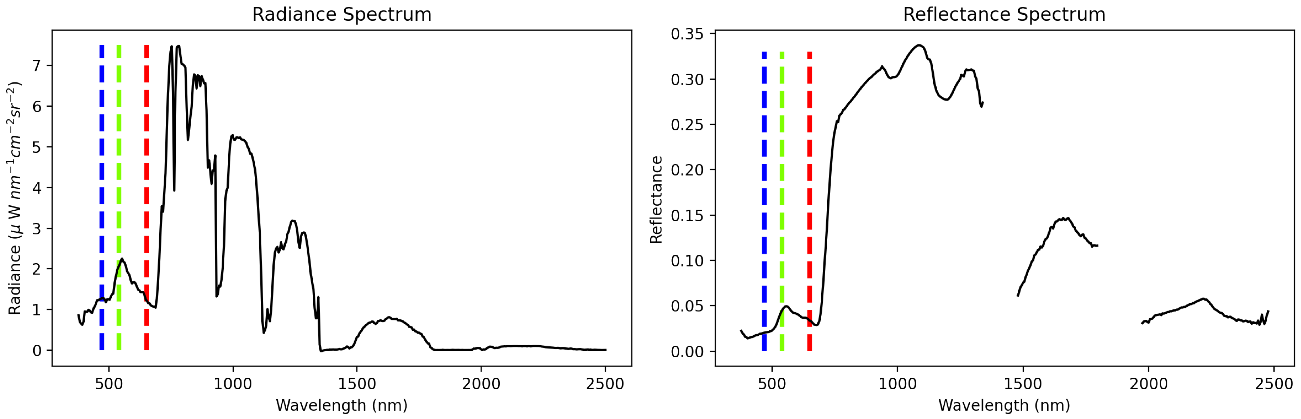
A representative radiance spectrum, and its associated reflectance, appear in Figure 1. The radiance spectrum represents energy incident at the detector per unit wavelength per solid angle per unit area, in units of W nm sr cm. Sharp dips at 940, 1140, 1380 and 1880 nm represent the influence of absorbing atmospheric gases HO, O, O, CO, and CH. The reflectance spectrum at right, showing the spectrum of a vegetated pixel, is comparatively smooth. Roughly speaking, it represents the ratio of light leaving the target over the light hitting the target, which is an intrinsic property of the surface. The deepest absorption features at 1380 and 1880 nm are not plotted; atmospheric gas absorption in these wavelengths is so strong that the atmosphere is opaque and it is not possible to estimate the surface reflectance. Mathematically, a single radiance observation y is a vector of intensity values corresponding to a set of wavelengths as measured by a remote sensor. The satellite radiance can be expressed as a function of the surface reflectance according to a forward model that takes into account atmospheric and physical effects, . We denote the joint surface and atmosphere state x, which combines the reflectance with additional components corresponding to atmospheric conditions . Optimal estimation [21] refers to the inversion of the forward model to compute the surface reflectance x given remotely sensed observations y and a prior assumption on x in a Bayesian context.
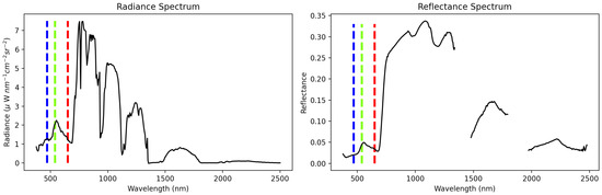
Figure 1.
Representative radiance and reflectance spectra. Red, green, and blue lines indicate visible color channels.
In this work, the additional components are aerosol optical depth (AOD) and column water vapor. The deterministic forward model is at the heart of the surface retrieval process and is briefly reviewed (Section 2.2) before describing the baseline retrievals (Section 2.3) and the details of the statistical model that will be relevant for our methodology (Section 2.4). This section is a summary of the statistical analysis described in Thompson et al. [23], which contains many additional details.
2.2. Forward Model and Uncertainty
The forward model is a nonlinear function describing the processes of absorption and scattering of light by atmospheric gases, particulates and clouds, and reflection by an underlying surface, and is referred to as the radiative transfer model (RTM). The true physical model is complicated, so many simplifying assumptions are used, such as treating surfaces as Lambertian (isotropic) rather than describing them using a bidirectional reflectance distribution function. Since there are many parameters to the RTM, optimization over all possible combinations is infeasible. Instead, a look-up table of optical coefficients is calculated in advance. This table, indexed by the atmospheric state, allows a fast calculation of the forward model in each channel [12]. Typical LUT values for our work follow a coarse grid of AOD values of [0.01, 0.1, 0.33, 0.66, 1.0] across H2O vapor levels of [1.0, 1.5, 2] g/cm, solved at each grid point via DISORT. Emulation is an emerging and promising alternative to a coarse LUT [29,30], but not taken advantage of in this work. Sensor elevations vary from 3000 to 6000 feet above ground, with ground elevation ranging from 8 to 1500 feet above sea level. The viewing zenith angle is set to 0 and the solar azimuth set to 180 degrees. Wavelengths range from 350 to 2520 nm with the REPTRAN fine band parameterization. Standardized “mid latitude” atmospheres for winter or summer are applied to all data and simulations. For a full description of the forward model assumptions, we refer the reader to previous work [31].
Uncertainties in the radiance prediction include instrument-related uncertainty such as measurement noise, as well as errors in atmospheric properties such as aerosol absorption or scattering. In the following experiments, we use the libRadtran radiative transfer library [11] with the ISOFIT inversion package [23]. This allows us to focus on the specific innovations of this paper, the prior specification and the optimization procedure.
2.3. Baseline Optimal Retrievals
As mentioned in the introduction, the baseline retrieval model assumes that any one observed radiance y with dimension 425 is a nonlinear function of a latent state x of dimension 427, independent of any nearby data: . The cardinality 425 represents the number of wavelengths that the AVIRIS-NG sensor can detect within the range of interest, while the latent state x includes the two atmospheric parameters. The forward model function described in the previous section is an approximation to the true physical system with higher-order complexities relegated to a Gaussian error term. The state x is given a Gaussian prior to provide a tractable posterior when combined with a linear approximation for the non-linear forward model:
The prior is discussed in the next section. The likelihood variance term for a single observation can be attributed to instrument noise and unobserved variables.
The optimal state vector is understood to be the retrieved vector that maximizes the posterior density , given prior assumptions and observations y. Negating, taking a logarithm, and dropping constants of the posterior yields a minimization problem with respect to a cost function :
The optimal estimate for the cost function Q can be found with the Newton-Raphson algorithm, which is an iterative method with update steps
However, the Hessian is expensive to compute. The linear approximation mentioned earlier is detailed in Appendix A.1 and results in a Gauss-Newton algorithm that yields an inexpensive update step of the form
In practice an additional diagonal term is added to the inverse term for better performance, so the Gauss-Newton algorithm becomes a Levenberg-Marquardt algorithm [32].
When the iterations converge to some state , the converged value represents the posterior mode, which can also be viewed as the mean of a Gaussian approximation to the posterior at the mode. The uncertainty is approximated with
The posterior is then approximated with the distribution , where the optimal estimate is with uncertainty .
2.4. Prior
In preparation for our spatial methodology, we detail the prior used for the baseline optimal estimation procedure. Recall that the prior state contains a surface state and an atmosphere state . The baseline method inverts each radiance measurement independently, and further assumes that the surface and atmosphere states are independent. This is represented with block diagonal covariances that make up a prior multivariate normal distribution:
The surface state components for a single radiance measurement can co-vary, as can the atmospheric state components; two prior states at different locations are however totally independent. Allowing different pixels to have co-varying atmospheric states will involve a cross-covariance function and is the focus starting with Section 2.5.
Natural and man-made materials have different reflectance profiles, so there are multiple prior means and variances , to take this into account. Note that there is a single global prior mean and variance for the atmospheric components. At the first iteration of the optimization routine, a heuristic algebraic inversion is used to estimate the reflectance, and then the closest prior is selected in an ad-hoc way using a Euclidean distance or Mahalonobis distance:
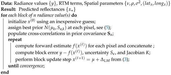
This prior is then fixed for subsequent iterations, and the optimization proceeds as outlined in Algorithm 1. For example, if the estimated reflectance at the first iteration is closest by distance to vegetation compared to concrete, water, or mud, a prior representing vegetation is used for computing the posterior until convergence. Although it is possible to update the prior with every iteration, this may prevent convergence. The parameters for the different priors are estimated with field observations made at Santa Barbara (UCSB) in California, USA and Hawaii, USA, see [23] for details. Ideally the prior could be computed with data from all over the world to account for the variety of vegetation and materials, which may lead to improved accuracy for both spatial and surface estimates. For the purpose of this work, the local data is adequate because our results are based on data collected in the same region.
| Algorithm 1: Simplified Optimal Spatial Inversion. |
 |
2.5. Naive Spatial Retrieval Structure
Extending the original model to a spatial model requires working with multiple observations at once. Following the notation earlier, let denote a single measurement and denote a collection of n concatenated measurements. Likewise for the state vector, let denote the set of state vectors to be retrieved with prior mean . In this notation, the spatial model takes the form
where , , all represent Kronecker product expansions of their non-spatial counterparts, and is an n-dimensional column vector of ones. Note that is applying the forward model to each corresponding state term. Each location may have a different prior for the surface component as described in Section 2.4, but for clarity we drop the k index from . As written, the model does not yet have spatial (cross-) correlations and is block diagonal. We introduce these correlations with off-diagonal elements, illustrated as follows for an example with :
We simplify the model by assuming the off diagonal blocks are all diagonal matrices, where denotes the covariance of the first atmospheric variable with itself at locations i and j. The off diagonal blocks could be full matrices, allowing for the different atmospheric parameters to influence each other. Estimating these cross-correlation parameters is feasible at a coarse scale with existing data sets [33], but is challenging and beyond the scope of this work.
To be precise, let denote the set of indices corresponding to the diagonal atmospheric components in the off-diagonal blocks of the prior cross covariance matrix, , so that in our case,
We can precisely specify the covariance matrix for a particular atmospheric variable. Denote the covariance for component k at locations as . Then the covariance matrix for the kth atmopsheric component across all locations, , is
In our situation, we only have two spatial atmospheric components, with and .
Concatenating the state and observed vectors and performing joint inference on the larger vector is a natural way to spatially extend a model, but may be inefficient for large samples, because we must invert the prior covariance as shown in (4). In the next section, we modify the specification to take advantage of the limited spatial structure.
2.6. Efficient Implementation
As described in Section 2.5, our spatial structure is restrictive in that each spatially correlated component only (spatially) interacts with itself and does not have cross-correlation with any other component. This independence can be exploited for scalability by writing the gradient descent step in terms of the non-spatial surface component for one pixel and the set of all atmospheric components. As before, let x denote the concatenated version of the latent state vector. For the update step shown in Equation (2) with representing the constant matrix that results from the Levenberg-Marquardt approximation in (A3), we have
with concatenated gradient term
where and are block diagonal. Hence, for pixel ,
where denotes the subvector of components corresponding to the th state vector. A key observation is that this subvector only depends on the th surface components , and atmospheric components and . In other words, retrieving the th state vector under spatial atmospheric effects does not cost much more than a non-spatial retrieval if the number of spatial components is small in comparison to the surface components. Furthermore, the block diagonal approach maintains some parallelizability of the original model. However, the block diagonal trick for efficiency does not carry over to estimating the posterior variance of the state vectors. This is because the block diagonal prior exploits the independence of the surface and atmospheric priors, while the forward model induces additional correlations in the posterior, see Equation (4).
2.7. Complexity
The computational complexity of our spatial procedure varies depending on the stage of the algorithm. Using the previous notation, the worst-case cost is due to the estimation of the posterior variance term shown in Equation (4). The problem is simple: although the matrices , K and can be written as block diagonal, the independent blocks of atmospheric and surface components in are correlated in , so we are forced to invert the entire matrix of dimension . In contrast, the worst case cost of the individual pixel inversions is , since we perform n inversions of a matrix.
However, if we are only interested in the posterior mean and approximate or precompute the Hessian term of Equation (6), the spatial model can have a cheaper update compared to the aggregate cost for the individual pixels. Letting s denote the number of spatial components, we have complexity per update step versus the for one update across independent pixels. Subtracting the two complexity terms, we see that when , or when the total number of pixels in the block is not too large, the spatial model has a lower cost since we have exploited the component-wise independence.
For example, in our simulation study we consider a nine pixel block inversions (n = 9) of roughly 400-dimensional prior states per pixel (p = 400), with two of the dimensions being atmospheric components (s = 2). Estimating the spatial posterior mean for a nine-pixel block then costs less than the individual means, given the term . To be clear, in this work we did not approximate the Hessian term in a way that reduces complexity.
Methods for significantly reducing the cubic complexity (from to nearly ) could be applied at multiple levels of the model and are explored in the Discussion as directions for future work.
2.8. Other Practical Considerations
Spatial models introduce additional parameters and effects that are not present for the original independent inversion procedure. For example, a common choice for the spatial correlation function and the one applied in this work is a Matérn covariance, which has a smoothness and range parameter. We provide one standard approach for estimating the Matérn parameters based on maximum likelihood in Appendix A.2, which we use in our application to real data. Some parameter choices lead to less stable computation than others; for example, using large range and smoothness parameters imply more strongly correlated components, which can lead to covariance matrices that are degenerate for the available machine precision. For our scenarios of interest, we have found that Matérn smoothness values near 1.5 and ranges between 500 and 1000 m are physically reasonable and numerically stable choices for the atmospheric components for the data collected by AVIRIS-NG. While using lower smoothness and range values are guaranteed to be stable, combinations of significantly higher values (such as smoothness of 3 and/or range of 5000 m) are expected to fail and are not recommended unless combined with other techniques that improve stability, such as a low rank approximation.
There are other, subtle effects that arise from the interplay between the data, the radiative transfer model (RTM), and the spatial correlation. Extreme values and sharp transitions in the atmosphere are smoothed by the spatial prior, and whether or not this smoothing is appropriate can depend on the source of the extreme values. For a point source of pollution (factory) or RTM convergence issues, the smoothing may increase error, while discrepancies from noise or smoke filled scenes may benefit from smoothing. A full accounting is beyond the scope of this work and we simply recommend the use of our model when it is safe to assume that the atmospheric components vary smoothly.
Post-hoc smoothing, or smoothing all of the atmospheric predictions after inversion as a post processing step, is a practically attractive smoothing approach that is decoupled from the radiative transfer model and hence fast and easy to implement. It inherits some of the issues of the spatial prior, in that parameters need to be estimated and smoothing may not always be appropriate, but fails to account for all of the correlations introduced by the RTM that are captured with a spatial prior. This results in lower predictive performance in a majority of cases and is illustrated in the next section.
3. Results
3.1. Simulation Study
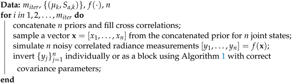
In this section, we present results of a simulation study, in which individual retrievals and their smoothed counterparts are compared to joint spatial retrievals. The simulation procedure consists of three high-level steps (Algorithm 2):
- Sample multiple surface reflectance states of vegetation, the most common of the priors described in Section 2.4. The atmospheric states are correlated according to their predetermined orientation following the technique outlined in Section 2.5.
- Simulate noisy AVIRIS-NG instrument radiance measurements corresponding to the sampled joint state using the built-in methods and configuration of the ISOFIT code [23]; the noise model is described in Section 2.2.
- Invert the simulated radiance measurements according to the implementation outlined in Section 2.6. Setting prior cross-pixel covariances to 0 results in individual retrievals as a special case.
For post-hoc smoothing, there is an additional post-processing step in which the independent estimates for the atmospheric components are treated as noisy samples from a latent smooth field; the noise is assumed to follow the posterior variance as computed by the individual inversions. This post-processed smooth field is estimated by kriging and uses the true data-generating covariance as a prior, which is the best-case scenario and better than could be expected in reality.
The input pixels are given evenly spaced locations with gaps fixed according to the number of pixels n for the 1D case. The 2D case uses a regular grid of pixels on the unit square. The spatial covariance function was taken to be Matérn with smoothness and range parameter values of for the 1D case and for the 2D case, to account for the greater distance between points. For context, the Matérn covariance generalizes more common choices like the exponential covariance (Matérn ) and squared exponential covariance (Matérn ); an intermediate value like is more realistic according to our analysis (see Appendix A.2). The variance parameters for the atmospheric components are 0.5 gcm for water vapor and 0.2 for AOD.
| Algorithm 2: Simulation Procedure: generate n pixels, compute correlated radiances, and invert. Repeat times. |
 |
While the sampled data were taken from a distribution with a realistic mean and covariance, it is important to note that there was no attempt to measure the realism of the samples themselves. Over a few hundred wavelengths, it is possible that many small variations accumulate to yield a simulated reflectance that is unlike any real surface. Furthermore, a realized latent atmospheric state could correspond to extreme conditions that require unique configuration. As a result, both inversion methods were prone to failing at individual points, adding noise to all of the simulated results. For example, out of five pixels, the second pixel may fail to converge; the resulting total error for the method across the five pixels would be larger, as the retrieved surface reflectance values may diverge for particular wavelengths and atmospheric components concentrate on boundary values. Under a spatial model, this error is then spread to the nearby points. To remedy the issue, we truncated the realizations to realistic values of g cm for vapor and for aerosol optical depth. These values are also similar to conditions under which real data is collected, so simulation results can better inform expectations with real data. Reducing the variance for the atmospheric components also helped avoid extreme realizations.
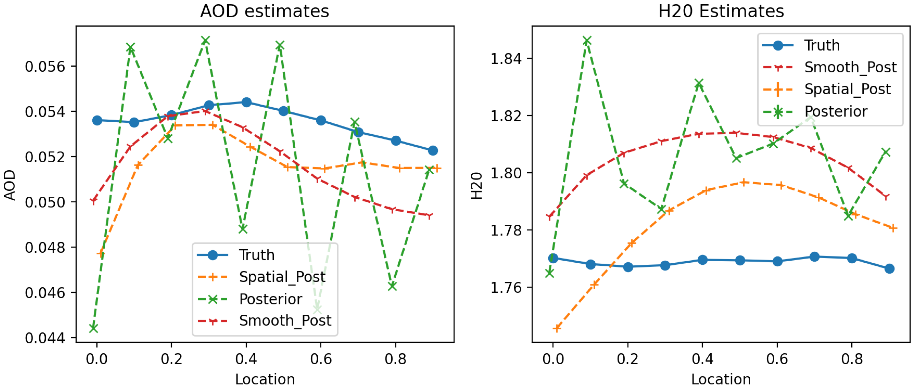
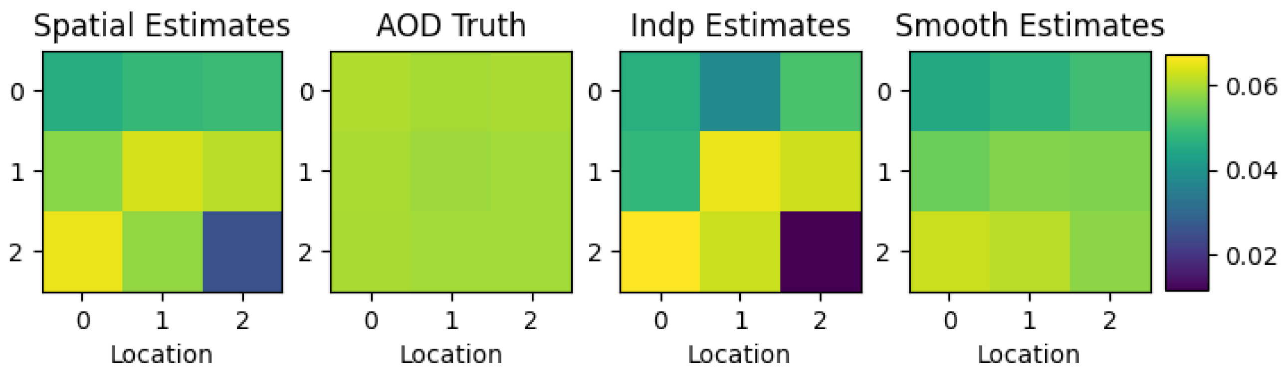
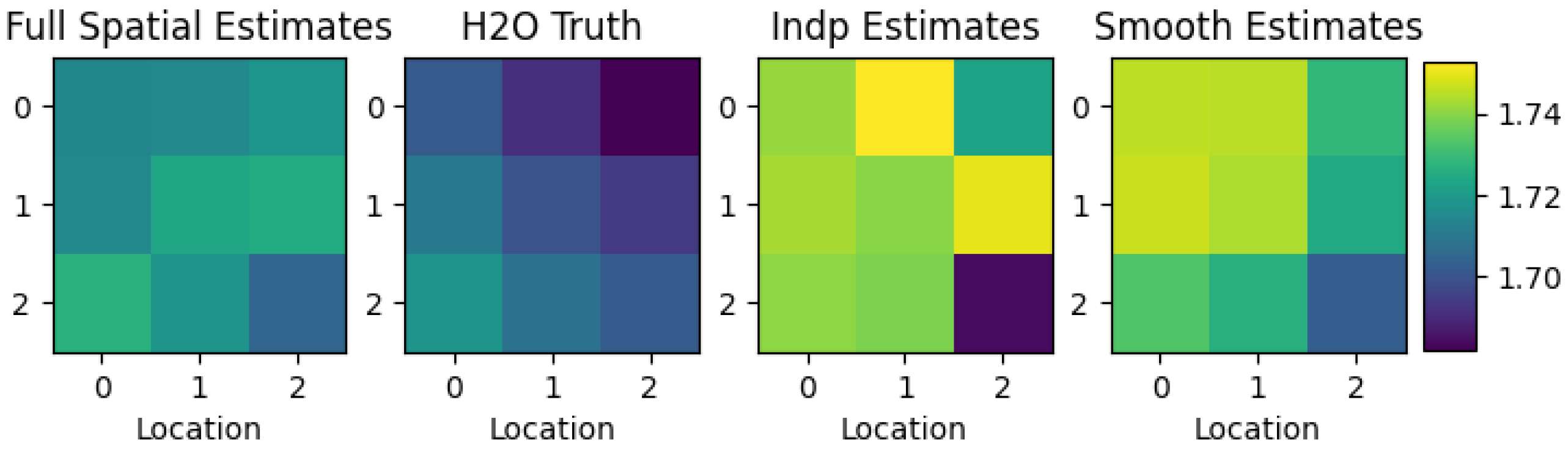
Figure 2, Figure 3 and Figure 4 illustrate the qualitative improvements that are possible with a spatial prior. While the independent inversions are at times closer to the truth, they may exhibit large oscillations that are avoided by the spatial retrievals due to the imposed correlation. In this way, the spatial inversions are more realistic. The post-hoc smoothing significantly improves upon the estimates of the independent inversions and yields results that are similar to the spatial prior in their realism. However, the smoothing cannot overcome large bias effects from the independent inversions.
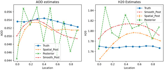
Figure 2.
Inversions of simulated data showing the water vapor (units of g/cm) and aerosol optical depth estimates across 10 pixels in 1D. The retrieved fields are more realistic for spatial (Spatial_Post) than for individual retrievals (Posterior). The post-hoc smoothing (Smooth_Post) can improve the individual retrievals but cannot overcome the bias.
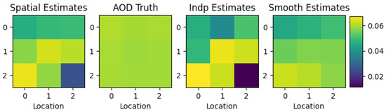
Figure 3.
Inversions of simulated data showing the aerosol optical depth estimates across 9 pixels on a grid. The spatial prior is more accurate than the independent inversions and comparable to post-hoc smoothing.

Figure 4.
Inversions of simulated data showing the water vapor estimates (units of g/cm) across 9 pixels on a grid. The spatial field better represents the truth; smoothing cannot overcome the bias in the independent estimates.
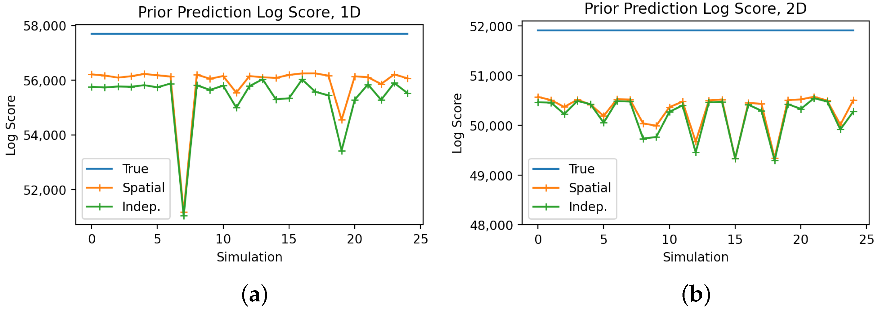
The mean square error is an unreliable indicator for inversion quality in the sense that highly variable components can inflate the MSE. Instead, we measure how closely the posterior mean reflects the true (prior) distribution with an ad-hoc “prior score”, and we quantify the predictive performance with the log score. The prior score simply estimates the log likelihood of the posterior mean given the prior, . Since the post-hoc smoothing does not change the prior, we do not compute the prior score for that case. The log score [34] is a proper score (e.g., [35]) that reflects how likely the simulated true data were under the estimated (Gaussian) predictive distribution, . It is important to note that the atmospheric components make up only two variables compared to the roughly 400 components of the reflectance per pixel inversion, so any improvements in log or prior scores are expected to be relatively small.
Figure 5a,b illustrate the prior score for the simulated realizations each of 1D and 2D pixel arrays. In most cases, the posterior is closer to the prior for the spatial case, resulting in a better prior score and implying that the spatial model better represents the data, as expected. For the 2D case, the difference is smaller, because of the greater inherent variability of a 2D field and the larger maximum distances between points.
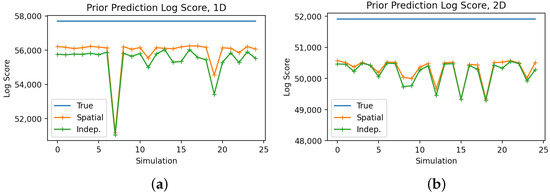
Figure 5.
Prior score plots for 25 simulated realizations. The posterior estimates for the spatial model are usually closer to their priors than the independent models. The effect is weaker for the 2D case, suggesting that the improvement tends to be most pronounced with highly correlated data. (a) Prior score results for a 1D array of 10 pixels. (b) Prior score results for a 2D grid of 9 pixels.
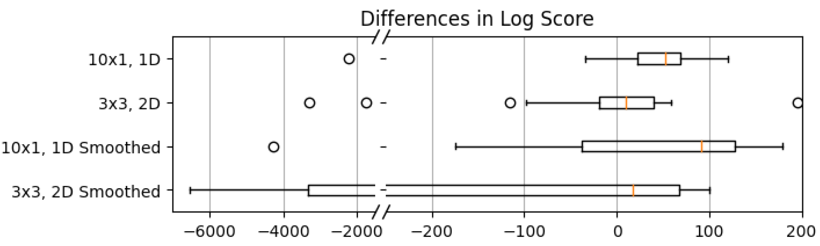
Figure 6 illustrates how the spatial inversion usually has better predictive performance compared to the individual inversions. The second set of boxes represent the difference between the spatial prior log scores and the post-hoc smoothing. Although the median is roughly unchanged, the other percentiles are inflated. The inflated lower percentile for the 2D log score difference suggests that when the individual estimates are not severely biased, the smoothing can drastically improve the predictive performance. However, when the individual estimates are biased, which is more often the case due to the positive median difference, the post-hoc smoothing cannot beat the smoothing induced with a spatial prior.
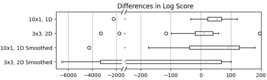
Figure 6.
The top box plots show the difference in log score between the spatial and independent models across 25 simulations. The quantile values are for the 1D case and for the 2D case. The two lower box plots show the difference in log score between the spatial and smoothed independent model. Quantiles are and for 1D and 2D respectively. Note the discontinuous x-axis.
3.2. Application to Real Data
We apply the spatial inversion to three sets of remotely sensed data from AVIRIS-NG. The current implementation of the inversion software, ISOFIT, produces pixelwise-independent estimates of surface reflectance and the two atmospheric components of water column vapor and aerosol optical thickness or depth (AOD), see Section 2.3. Measurements were taken by plane from 5 to 10 km altitude and were orthocorrected for plane movement.
Before applying the methodology to real data, we estimate the covariance parameters of the spatial model with a field of water vapor measurements estimated by the independent inversion procedure on an unrelated data set in India. Our chosen parameter values for both water vapor and aerosols were: a range m, smoothness , a nugget effect of 0.001 and variance . The procedure and justification for this choice are presented in Appendix A.2.
The first data set we consider is a validation measurement taken at Ivanpah Playa in California, USA on 28 March 2017 at about 5:30 p.m. Ideally the data set would consist of AVIRIS-NG observations along with multiple simultaneous measurements of in situ aerosols and water vapor over the region, which would allow for validation of the method as in [23]. Since a data set like this does not currently exist, the Ivanpah data set with just a single, area-wide measurement for the aerosols and vapor is the best available alternative. The weather conditions for the measurement are extremely uniform and clear, so we perform a spatial inversion to determine if the noise in the atmospheric components is smoothed.
The results of the validation show that the atmospheric components can have slightly less bias under the spatial model, but the effect is practically insignificant. The in situ measured aerosol optical thickness and water vapor are roughly 0.043 and 0.88, respectively. The estimates for aerosols shown in Figure 7 vary from 0.01 to 0.012, which underestimates the in-situ measurement of 0.043, but in practice the difference is negligible as AOD values up to 0.05 correspond to extremely clear skies. The water vapor measurements are nearly identical and uniformly valued at 0.67 for all methods, which also underestimates the in situ measurements of 0.88. Such differences of 0.2 g cm are not unrealistic, since the in situ measurement carries its own uncertainty and the optical absorption path of the two instruments is different. Together, this validation study confirms that a spatial model does no harm and can help lower the overall error of the aerosol estimates, but the spatial error for such homogeneous scenes is negligible.

Figure 7.
The aerosol optical depth prediction for validation data at Ivanpah. The predictions are effectively identical, but the spatial retrievals are closer to the in situ measurement of 0.043.
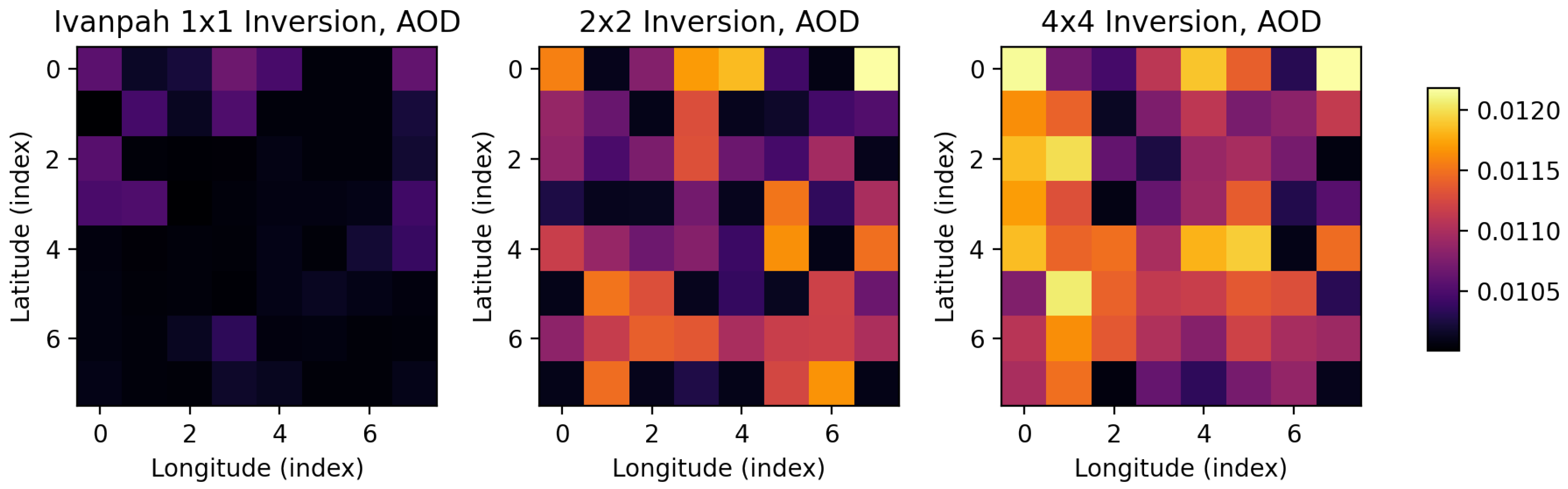
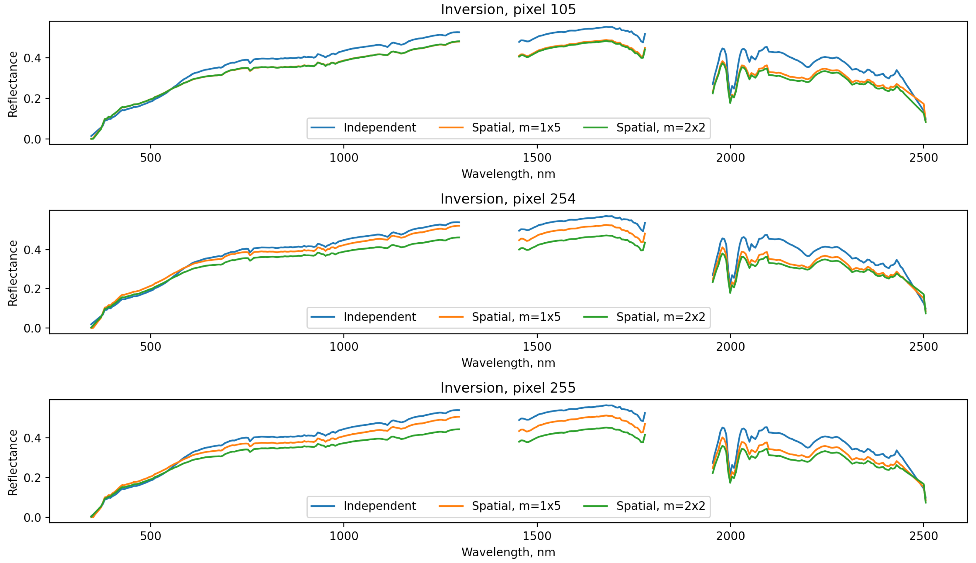
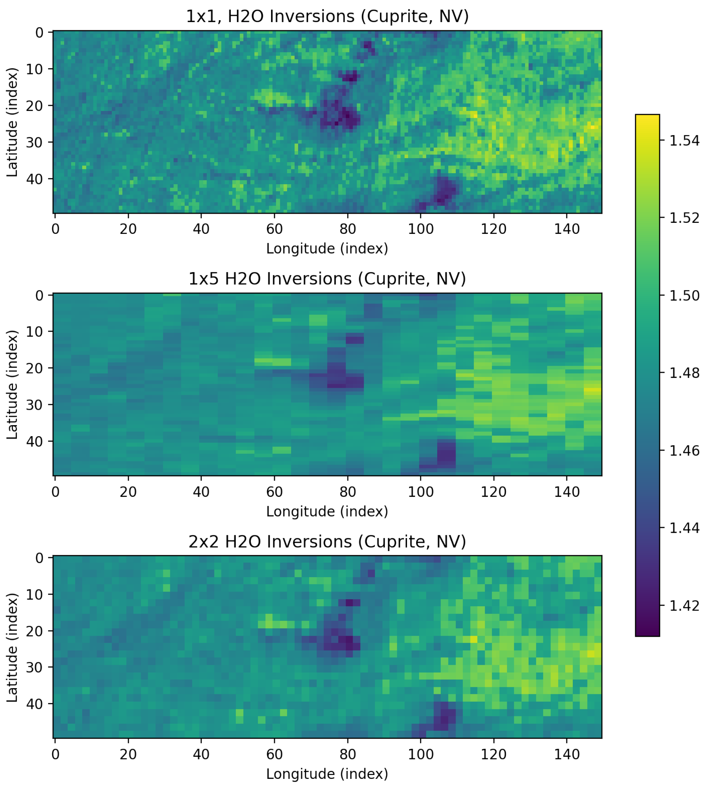
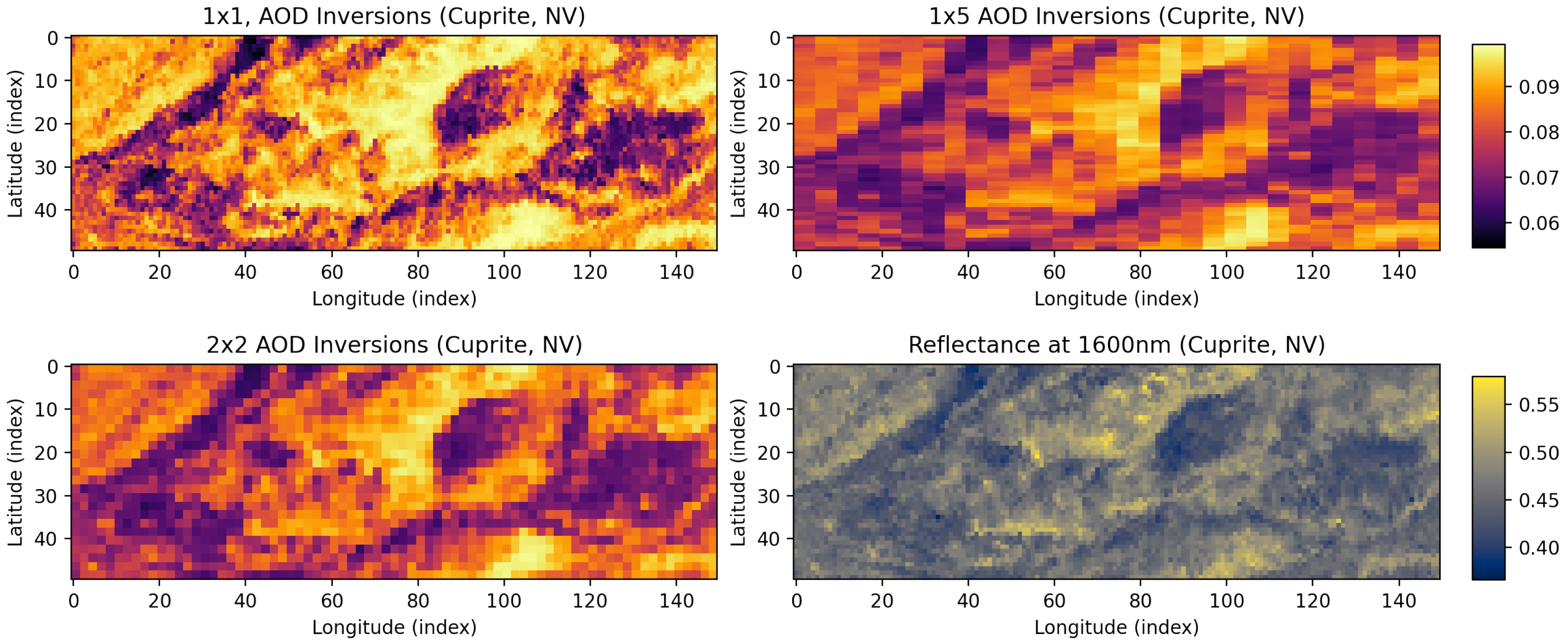
The next data set we explored was measured on 25 June 2014 at roughly 7:30 p.m. local time over Cuprite Hills in Nevada, USA. Here we have a swath of 50 × 150 pixels and perform individual, 1 × 5 pixel inversions, and 2 × 2 pixel inversions, with the spatial inversions using the same Matérn parameters (1.5, 0.75) as the previous data set. The choice of 1 × 5 and 2 × 2 pixels helps illustrate the difference between a 1-dimension, push-broom type of correlation versus a 2-dimensional correlation. We find very little difference in the surface reflectance across pixels shown in Figure 8. There is a mild scaling effect that occurs with the spatial versions, which we attribute to the different results for the atmospheric components, but the shape is consistently characteristic of soil with minerals. The results for atmospheric water vapor shown in Figure 9 show that the spatial models provide a smoothing effect that reduces the noisy estimates of the independent inversions. The aerosol optical thickness in Figure 10 has a similar story, where the spatial values tend to be lower and smoother than the independent inversion, which has stronger gradients between pixels. The fourth subfigure of Figure 10 shows reflectance for an arbitrary wavelength and suggests that the aerosols detected by all methods are influenced by the land reflectance, with the independent inversions more strongly influenced compared to the spatial methods.
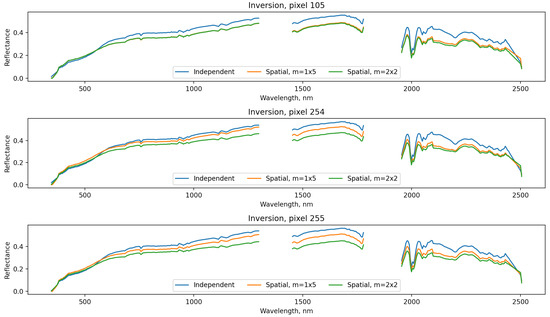
Figure 8.
The surface reflectance profiles are nearly identical for the Cuprite data, with scaling changes due to the estimation of atmospheric parameters. This suggests that independent inversions may be overestimating reflectance. Pixels 105, 254, and 255 are adjacent and the reflectance can be interpreted as a percent, so at a particular wavelength a reflectance of 0.4 means 40% of the incoming radiant energy is reflected.
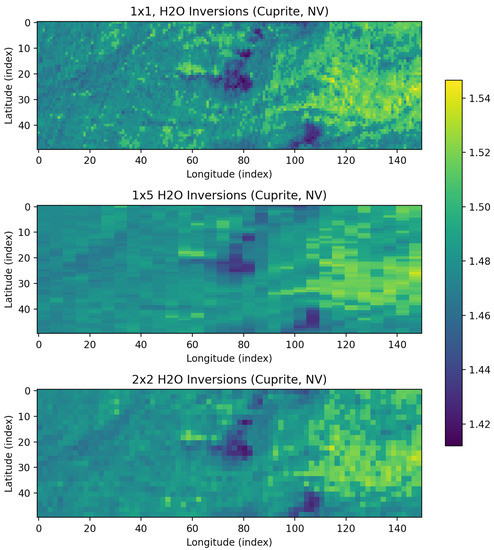
Figure 9.
The water vapor (units of g/cm) estimates are noticeably smoother under the spatial models. The predicted fields are qualitatively more realistic and are a principled alternative to post-hoc smoothing.
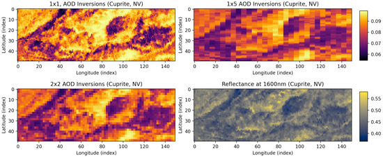
Figure 10.
For the Cuprite dataset, the aerosol optical depth prediction is susceptible to the surface state prediction (bottom right), but smoothing with a spatial prior decreases the noise. The top left figure shows inversions done 1 pixel at a time, compared to stripes of 1 × 5 pixels in the top right figure and squares of 2 × 2 pixels in the bottom left figure. The bottom right figure shows topography visible at a single wavelength, 1600 nm.
Our last data set was collected over Yolo in California, USA on the outskirts of Sacramento, California on 7 September 2020 at about 7 p.m. The conditions for this data set were smoky: wildfires had increased the amount of aerosols in the atmosphere and varying amounts of smoke are visible in the color images of the scene. We invert a coarse grid over the entire scene to see if the recovered aerosol states can capture the smoothly varying field suggested by the imagery. The full swath is about 2500 × 500 pixels, so we subsample every 25th pixel with a buffer from the edges to get 94 × 16 inversions.
Figure 11 shows a comparison of the independent and a 2 × 2 inversion. While the HO predictions were nearly identical, the aerosol field was significantly smoothed. There are a few areas in the spatial model that appear to be outliers but may be explained as the spatial model spreading the effect of large individual pixel values for the aerosols. It is expected that inverting a larger collection of pixels simultaneously (for example, 10 × 10) will result in the large values being spread out even more and higher overall estimates for the aerosol field. Combined with the results of the validation data at Ivanpah, the spatial model may counteract or provide lower bias for atmospheric components compared to independent inversions.
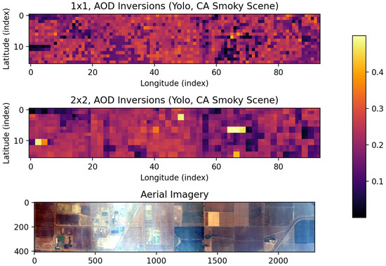
Figure 11.
A retrieved aerosol field under a spatial model is smoother than the independent retrievals and spreads out large estimates.
4. Discussion
We illustrated the mathematical details and addressed the basic computation challenges that arise when performing spatial retrievals with the introduction of cross-correlation with a Gaussian process prior. The block independent implementation we chose is both simple and allows for straightforward parallelization, but can exhibit a computational complexity that is cubic in cardinality of the block. Our simulations showed that a spatial radiative transfer model offers a better log score when compared to the non-spatial version. In particular, the log score plot reveals that most simulations benefit from a spatial approach, but in some cases the simple techniques perform very well. With real satellite data, we demonstrated how the spatial model can offer qualitatively improved retrievals with lower perceived error in the the atmospheric components. However, we note that the estimates of surface reflectance were not significantly affected.
Although we do not have spatially varying situ measurements to compute accuracy scores for real data, we showed that the spatial model does provide additional smoothing to the atmospheric components, resulting in more realistic predictions for the atmospheric state across space. We also noticed a consistent trend in which the spatial models show slightly less bias in the atmospheric components. This is particularly important when comparing to post smoothing methods, which can greatly improve individual atmospheric estimates but cannot overcome bias. Future work would benefit from a true verification data set, which could be used to generate more realistic simulated sets of surface pixels. The atmospheric component of the simulations could be made far more sophisticated by leveraging meteorological models.
While we recommend this methodology for cases where the atmosphere is not ideal, more simulation and data analysis would be needed to quantify the range of atmospheric conditions under which there is a significant advantage for our method. We showed how very clear atmospheric conditions such as those in the Ivanpah data set do not get any practical benefit. Data sets under very smoky or moist atmospheres show more potential, but at present they are less common and need to be collected under different combinations. This analysis should also elucidate what size and shape pixel block is best. For example, very large pixel blocks may induce too much smoothing when there are sharp changes in atmospheric conditions. Alternatively, choosing blocks that consist of a smaller number of spread out pixels could increase the chance of having contrasting surfaces that may better reveal the atmospheric state as oppose to a more uniform set of surfaces. These myriad tasks were beyond the scope of this work.
From a development point of view, a next step is to apply one of the many spatial approximations to allow for efficient, simultaneous inversion of larger data sets. Inducing sparsity in precision matrices (e.g., [36,37,38]) or low-rank approaches [39,40,41] stand out as the best options. The correlation structure could also be extended to include quantities such as elevation or terrain effects, rather than just latitude and longitude, to take into account possible discontinuities or interactions between topography and the atmosphere. From an application point of view, essentially any inversion that involves smoothly varying components can be extended with this methodology. One special case is exoplanet surface analysis, in which the exoplanet surface is expected to have some type of atmosphere and even a very simple atmospheric model may lead to improved retrievals. Alternately, a spatial model for the local atmosphere offers telluric corrections on upward-looking observation time series of exoplanet spectra from a ground-based spectrometer. The “surface” of interest may be a star, and the local atmosphere can be modeled as a 1-D Gaussian Markov system where belief propagation gives a tractable exact solution. Correlations over the temporal domain can be included as well if there are multiple reflectances measured over time.
In addition to using approximations for the spatial prior, further speed-ups might be obtained by GP emulation of the forward model after dimension reduction via active subspace on the latent state and functional PCA on the observations. The data model may be improved by considering the radiance measurement as a count, implying a Poisson or generalized linear model where the variance is equal to the mean, rather than a Gaussian model. An alternative is to assume a log Gaussian model for the observations, which would avoid some of the additional computational burden of a Poisson model.
Aside from improving the efficiency of the algorithm, the model itself could be modified to account for adjacency effects, which are assumed negligible in this work. Given a priori knowledge or an initial run to determine that surface states are of similar nature, the reflectance of those locations can be re-estimated with correlated surfaces. This correlation between surfaces could be combined with that atmospheric correlations to take into account all possible local correlations.
5. Conclusions
In this work we showed how to account for spatial correlations in retrievals of surface reflectance from imaging spectroscopic measurements. The standard methodology inverts a single radiance measurement to estimate surface reflectance and atmospheric states of aerosols and water vapor. By directly modeling the physical correlations of the atmospheric components, we can invert multiple measurements simultaneously and borrow strength from nearby locations to get more robust predictions of the non-spatial reflectances. In contrast, kriging or post-processing the fields to create smoothness does not take into account the dependencies between variables induced by the nonlinear model and would result in inaccurate fields.
Author Contributions
Conceptualization, J.H. and M.K.; methodology, D.R.T. and M.K.; software, D.R.T. and D.Z.; validation, D.R.T. and D.Z.; formal analysis, D.Z.; investigation, D.Z.; writing—original draft preparation, M.K., V.N., D.R.T. and J.H.; visualization, D.Z.; writing—review and editing, D.Z.; supervision, J.H., D.R.T. and M.K.; project administration, J.H. and A.B.; funding acquisition, J.H. and M.K. All authors have read and agreed to the published version of the manuscript.
Funding
This research was partially supported by the Research and Technology Development Fund of the Jet Propulsion Laboratory, California Institute of Technology. MK was also partially supported by National Science Foundation (NSF) Grants DMS–1521676, DMS–1654083, and DMS–1953005. Portions of this work were performed at the Jet Propulsion Laboratory, California Institute of Technology, under contract with NASA.
Data Availability Statement
Not applicable.
Conflicts of Interest
The authors declare no conflict of interest.
Abbreviations
The following abbreviations are used in this manuscript:
| VSWIR | Visible/Shortwave InfraRed |
| AVIRIS-NG | Airborne Visible-Infrared Imaging Spectrometer-Next Generation |
| ATREM | Atmosphere Removal |
| LUT | Look-up Table |
| UQ | Uncertainty Quantification |
| OE | Optimal Estimation |
| AOD | Aerosol Optical Depth |
| RTM | Radiative Transfer Model |
Appendix A. Appendix/Proofs
Appendix A.1. Iterative Optimization
The optimization algorithm iteratively solves for the value x that minimizes a cost, , by using the approximation , where we have denoted the Jacobian . Differentiating with respect to x and setting to 0 gives the Gauss-Newton update of . Substituting with , where is a positive diagonal matrix specified later, results in a Levenberg-Marquardt update.
In our context, the cost function is slightly more general:
Substituting the second order approximation where and noting the Jacobian now has two terms, we initially follow a Gauss-Newton algorithm as follows. Starting from a rearranged cost,
the Jacobian can be thought of as a coefficient vector J applied to a residual vector R:
The residual is represented by two different reference points: the expansion point and the prior mean . It is not obvious how to plug the Jacobian and residual terms into the Gauss-Newton update step, so we manually compute the gradient of the loss,
and set it to zero and collect terms to get the update step. We denote the Hessian as .
The iteration continues with as the next expansion point. For arbitrary iteration around , we recover the update step shown in Section 2.3
where . The likelihood that corresponds to the first order approximation is
Recalling that the prior is , it is simple to show that each step of the algorithm as shown in Equation (A3) is the posterior expectation:
where the posterior is . To improve performance, the diagonal term may be added to the Hessian, resulting in a Levenberg-Marquardt algorithm. This Hessian approximation is represented as in Equation (6).
Appendix A.2. Parameter Estimation
We estimated Matérn smoothness and range parameters for water vapor using measurements collected by AVIRIS-NG over Desalpar in India on 25 March 2018 at roughly 7 a.m. We used a cross-validation-type procedure in which we maximize the predictive likelihood (related to the log score) of a set of test points given a posterior computed from a set of training points. The data set was roughly 3000 by 500 pixels, so we used a training set lattice of 300 by 50 pixels (subsampling every tenth pixel) and a test set defined by offsetting the training set by five pixels. Given the cubic complexity when computing likelihoods for a Gaussian process, we utilize the GPVecchia package to perform efficient (linear in sample size, [38]) computation of the likelihood with a nearest-neighbor approximation.
The estimation of both range and smoothness parameters simultaneously was unstable, so we iteratively optimized the parameters one at a time until the change in each parameter value was less than a threshold, one percent in our case. Initializing the procedure with smoothness 1.5, range 5 (measured in pixels), with variance fixed to 1, and a nugget (representing noise) of 0.01, we converged to a range of 146.49 pixels and smoothness of 1.411. The pixel size for this data set is recorded as 5 m, hence the range can be interpreted as about 750 m. Since the Matérn covariance has a very efficient form for smoothness values of 1.5, we rounded to that value for all computations. For simplicity, we assumed the aerosol field to have the same spatial covariance parameters.
References
- Space Studies Board; National Academies of Sciences, Engineering, and Medicine. Thriving on Our Changing Planet: A Decadal Strategy for Earth Observation from Space; National Academies Press: Washington, DC, USA, 2019. [Google Scholar]
- Chapman, J.W.; Thompson, D.R.; Helmlinger, M.C.; Bue, B.D.; Green, R.O.; Eastwood, M.L.; Geier, S.; Olson-Duvall, W.; Lundeen, S.R. Spectral and radiometric calibration of the next generation airborne visible infrared spectrometer (AVIRIS-NG). Remote Sens. 2019, 11, 2129. [Google Scholar] [CrossRef] [Green Version]
- Cogliati, S.; Sarti, F.; Chiarantini, L.; Cosi, M.; Lorusso, R.; Lopinto, E.; Miglietta, F.; Genesio, L.; Guanter, L.; Damm, A.; et al. The PRISMA imaging spectroscopy mission: Overview and first performance analysis. Remote Sens. Environ. 2021, 262, 112499. [Google Scholar] [CrossRef]
- Guanter, L.; Kaufmann, H.; Segl, K.; Foerster, S.; Rogass, C.; Chabrillat, S.; Kuester, T.; Hollstein, A.; Rossner, G.; Chlebek, C.; et al. The EnMAP spaceborne imaging spectroscopy mission for earth observation. Remote Sens. 2015, 7, 8830–8857. [Google Scholar] [CrossRef] [Green Version]
- Connelly, D.S.; Thompson, D.R.; Mahowald, N.M.; Li, L.; Carmon, N.; Okin, G.S.; Green, R.O. The EMIT mission information yield for mineral dust radiative forcing. Remote Sens. Environ. 2021, 258, 112380. [Google Scholar] [CrossRef]
- Nieke, J.; Rast, M. Towards the copernicus hyperspectral imaging mission for the environment (CHIME). In Proceedings of the Igarss 2018–2018 IEEE International Geoscience and Remote Sensing Symposium, Valencia, Spain, 22–27 July 2018; IEEE: Piscataway, NJ, USA, 2018; pp. 157–159. [Google Scholar]
- Alonso, K.; Bachmann, M.; Burch, K.; Carmona, E.; Cerra, D.; De los Reyes, R.; Dietrich, D.; Heiden, U.; Hölderlin, A.; Ickes, J.; et al. Data products, quality and validation of the DLR earth sensing imaging spectrometer (DESIS). Sensors 2019, 19, 4471. [Google Scholar] [CrossRef] [PubMed] [Green Version]
- Yokoya, N.; Iwasaki, A. Hyperspectral and multispectral data fusion mission on hyperspectral imager suite (HISUI). In Proceedings of the 2013 IEEE International Geoscience and Remote Sensing Symposium-IGARSS, Melbourne, VIC, Australia, 21–26 July 2013; IEEE: Piscataway, NJ, USA, 2013; pp. 4086–4089. [Google Scholar]
- Schaepman-Strub, G.; Schaepman, M.E.; Painter, T.H.; Dangel, S.; Martonchik, J.V. Reflectance quantities in optical remote sensing—Definitions and case studies. Remote Sens. Environ. 2006, 103, 27–42. [Google Scholar] [CrossRef]
- Berk, A.; Conforti, P.; Kennett, R.; Perkins, T.; Hawes, F.; Van Den Bosch, J. MODTRAN® 6: A major upgrade of the MODTRAN® radiative transfer code. In Proceedings of the 2014 6th Workshop on Hyperspectral Image and Signal Processing: Evolution in Remote Sensing (WHISPERS), Lausanne, Switzerland, 24–27 June 2014; IEEE: Piscataway, NJ, USA, 2014; pp. 1–4. [Google Scholar]
- Emde, C.; Buras-Schnell, R.; Kylling, A.; Mayer, B.; Gasteiger, J.; Hamann, U.; Kylling, J.; Richter, B.; Pause, C.; Dowling, T.; et al. The libRadtran software package for radiative transfer calculations (version 2.0. 1). Geosci. Model Dev. 2016, 9, 1647–1672. [Google Scholar] [CrossRef] [Green Version]
- Thompson, D.R.; Guanter, L.; Berk, A.; Gao, B.C.; Richter, R.; Schläpfer, D.; Thome, K.J. Retrieval of atmospheric parameters and surface reflectance from visible and shortwave infrared imaging spectroscopy data. Surv. Geophys. 2019, 40, 333–360. [Google Scholar] [CrossRef] [Green Version]
- Gao, B.C.; Montes, M.J.; Li, R.R.; Dierssen, H.M.; Davis, C.O. An atmospheric correction algorithm for remote sensing of bright coastal waters using MODIS land and ocean channels in the solar spectral region. IEEE Trans. Geosci. Remote Sens. 2007, 45, 1835–1843. [Google Scholar] [CrossRef]
- Thompson, D.R.; Gao, B.C.; Green, R.O.; Roberts, D.A.; Dennison, P.E.; Lundeen, S.R. Atmospheric correction for global mapping spectroscopy: ATREM advances for the HyspIRI preparatory campaign. Remote Sens. Environ. 2015, 167, 64–77. [Google Scholar] [CrossRef]
- Healey, G.; Slater, D. Models and methods for automated material identification in hyperspectral imagery acquired under unknown illumination and atmospheric conditions. IEEE Trans. Geosci. Remote Sens. 1999, 37, 2706–2717. [Google Scholar] [CrossRef] [Green Version]
- Acito, N.; Diani, M.; Corsini, G. Coupled subspace-based atmospheric compensation of LWIR hyperspectral data. IEEE Trans. Geosci. Remote Sens. 2019, 57, 5224–5238. [Google Scholar] [CrossRef]
- Guanter, L.; Del Carmen González-Sanpedro, M.; Moreno, J. A method for the atmospheric correction of ENVISAT/MERIS data over land targets. Int. J. Remote Sens. 2007, 28, 709–728. [Google Scholar] [CrossRef]
- Cressie, N. Statistics for Spatial Data, Revised Edition; John Wiley & Sons: New York, NY, USA, 1993. [Google Scholar]
- Thompson, D.R.; Kahn, B.H.; Brodrick, P.G.; Lebsock, M.D.; Richardson, M.; Green, R.O. Spectroscopic Imaging of Sub-Kilometer Spatial Structure in Lower Tropospheric Water Vapor. Atmos. Meas. Tech. 2021, 14, 2827–2840. [Google Scholar] [CrossRef]
- Rodgers, C.D. Retrieval of atmospheric temperature and composition from remote measurements of thermal radiation. Rev. Geophys. 1976, 14, 609–624. [Google Scholar] [CrossRef]
- Rodgers, C.D. Inverse Methods for Atmospheric Sounding: Theory and Practice; World Scientific: Singapore, 2000; Volume 2. [Google Scholar]
- Mouroulis, P.Z. Spectral and spatial uniformity in pushbroom imaging spectrometers. In Proceedings of the Imaging Spectrometry V. International Society for Optics and Photonics, Denver, CO, USA, 18–23 July 1999; Volume 3753, pp. 133–141. [Google Scholar]
- Thompson, D.R.; Natraj, V.; Green, R.O.; Helmlinger, M.C.; Gao, B.C.; Eastwood, M.L. Optimal estimation for imaging spectrometer atmospheric correction. Remote Sens. Environ. 2018, 216, 355–373. [Google Scholar] [CrossRef]
- Dubovik, O.; Herman, M.; Holdak, A.; Lapyonok, T.; Tanré, D.; Deuzé, J.; Ducos, F.; Sinyuk, A.; Lopatin, A. Statistically optimized inversion algorithm for enhanced retrieval of aerosol properties from spectral multi-angle polarimetric satellite observations. Atmos. Meas. Tech. 2011, 4, 975–1018. [Google Scholar] [CrossRef] [Green Version]
- Xu, F.; Diner, D.J.; Dubovik, O.; Schechner, Y. A correlated multi-pixel inversion approach for aerosol remote sensing. Remote Sens. 2019, 11, 746. [Google Scholar] [CrossRef] [Green Version]
- Hobbs, J.; Katzfuss, M.; Zilber, D.; Brynjarsdóttir, J.; Mondal, A.; Berrocal, V. Spatial retrievals of atmospheric carbon dioxide from satellite observations. Remote Sens. 2021, 13, 571. [Google Scholar] [CrossRef]
- Diner, D.J.; Martonchik, J.V.; Kahn, R.A.; Pinty, B.; Gobron, N.; Nelson, D.L.; Holben, B.N. Using angular and spectral shape similarity constraints to improve MISR aerosol and surface retrievals over land. Remote Sens. Environ. 2005, 94, 155–171. [Google Scholar] [CrossRef]
- Lyapustin, A.; Wang, Y.; Laszlo, I.; Kahn, R.; Korkin, S.; Remer, L.; Levy, R.; Reid, J. Multiangle implementation of atmospheric correction (MAIAC): 2. Aerosol algorithm. J. Geophys. Res. Atmos. 2011, 116. [Google Scholar] [CrossRef]
- Servera, J.V.; Rivera-Caicedo, J.P.; Verrelst, J.; Muñoz-Marí, J.; Sabater, N.; Berthelot, B.; Camps-Valls, G.; Moreno, J. Systematic Assessment of MODTRAN Emulators for Atmospheric Correction. IEEE Trans. Geosci. Remote Sens. 2021, 60, 1–17. [Google Scholar] [CrossRef]
- Brodrick, P.G.; Thompson, D.R.; Fahlen, J.E.; Eastwood, M.L.; Sarture, C.M.; Lundeen, S.R.; Olson-Duvall, W.; Carmon, N.; Green, R.O. Generalized radiative transfer emulation for imaging spectroscopy reflectance retrievals. Remote Sens. Environ. 2021, 261, 112476. [Google Scholar] [CrossRef]
- Thompson, D.R.; Braverman, A.; Brodrick, P.G.; Candela, A.; Carmon, N.; Clark, R.N.; Connelly, D.; Green, R.O.; Kokaly, R.F.; Li, L.; et al. Quantifying uncertainty for remote spectroscopy of surface composition. Remote Sens. Environ. 2020, 247, 111898. [Google Scholar] [CrossRef]
- Ranganathan, A. The levenberg-marquardt algorithm. Tutoral LM Algorithm 2004, 11, 101–110. [Google Scholar]
- Kinne, S. The MACv2 aerosol climatology. Tellus B Chem. Phys. Meteorol. 2019, 71, 1–21. [Google Scholar] [CrossRef] [Green Version]
- Gneiting, T.; Raftery, A.E. Strictly proper scoring rules, prediction, and estimation. J. Am. Stat. Assoc. 2007, 102, 359–378. [Google Scholar] [CrossRef]
- Gneiting, T.; Katzfuss, M. Probabilistic forecasting. Annu. Rev. Stat. Appl. 2014, 1, 125–151. [Google Scholar] [CrossRef]
- Lindgren, F.; Rue, H.; Lindström, J. An explicit link between Gaussian fields and Gaussian Markov random fields: The stochastic partial differential equation approach. J. R. Stat. Soc. Ser. B 2011, 73, 423–498. [Google Scholar] [CrossRef] [Green Version]
- Nychka, D.W.; Bandyopadhyay, S.; Hammerling, D.; Lindgren, F.; Sain, S.R. A multi-resolution Gaussian process model for the analysis of large spatial data sets. J. Comput. Graph. Stat. 2015, 24, 579–599. [Google Scholar] [CrossRef] [Green Version]
- Katzfuss, M.; Guinness, J. A general framework for Vecchia approximations of Gaussian processes. Stat. Sci. 2021, 36, 124–141. [Google Scholar] [CrossRef]
- Quiñonero-Candela, J.; Rasmussen, C.E. A unifying view of sparse approximate Gaussian process regression. J. Mach. Learn. Res. 2005, 6, 1939–1959. [Google Scholar]
- Banerjee, S.; Gelfand, A.E.; Finley, A.O.; Sang, H. Gaussian predictive process models for large spatial data sets. J. R. Stat. Soc. Ser. B 2008, 70, 825–848. [Google Scholar] [CrossRef] [PubMed] [Green Version]
- Katzfuss, M.; Cressie, N. Spatio-temporal smoothing and EM estimation for massive remote-sensing data sets. J. Time Ser. Anal. 2011, 32, 430–446. [Google Scholar] [CrossRef]

Publisher’s Note: MDPI stays neutral with regard to jurisdictional claims in published maps and institutional affiliations. |
© 2022 by the authors. Licensee MDPI, Basel, Switzerland. This article is an open access article distributed under the terms and conditions of the Creative Commons Attribution (CC BY) license (https://creativecommons.org/licenses/by/4.0/).