Abstract
Kelp forests are commonly classified within remote sensing imagery by contrasting the high reflectance in the near-infrared spectral region of kelp canopy floating at the surface with the low reflectance in the same spectral region of water. However, kelp canopy is often submerged below the surface of the water, making it important to understand the effects of kelp submersion on the above-water reflectance of kelp, and the depth to which kelp can be detected, in order to reduce uncertainties around the kelp canopy area when mapping kelp. Here, we characterized changes to the above-water spectra of Nereocystis luetkeana (Bull kelp) as different canopy structures (bulb and blades) were submerged in water from the surface to 100 cm in 10 cm increments, while collecting above-water hyperspectral measurements with a spectroradiometer (325–1075 nm). The hyperspectral data were simulated into the multispectral bandwidths of the WorldView-3 satellite and the Micasense RedEdge-MX unoccupied aerial vehicle sensors and vegetation indices were calculated to compare detection limits of kelp with a focus on differences between red edge and near infrared indices. For kelp on the surface, near-infrared reflectance was higher than red-edge reflectance. Once submerged, the kelp spectra showed two narrow reflectance peaks in the red-edge and near-infrared wavelength ranges, and the red-edge peak was consistently higher than the near-infrared peak. As a result, kelp was detected deeper with vegetation indices calculated with a red-edge band versus those calculated with a near infrared band. Our results show that using red-edge bands increased detection of submerged kelp canopy, which may be beneficial for estimating kelp surface-canopy area and biomass.
1. Introduction
Kelp forests are highly productive three-dimensional coastal marine habitats [1,2] that provide a number of environmental services and contribute substantial economic value to coastal communities globally [3]. In the northeast Pacific, the two dominant surface-canopy forming kelp species, Nereocystis luetkeana and Macrocystis pyrifera [4], stabilize shorelines via wave dampening [5,6], support economically important fisheries [7,8], and are commercially harvested for various purposes [9,10]. However, both kelp species are subject to high spatial and temporal variability, correlated with biotic and abiotic drivers of change [11,12]. As such, resource managers are incentivized to monitor the status of these kelp forests, and the corollary effects of the ecosystem services they provide [10,12,13], a task that has been facilitated by remote sensing since the mid-20th century [12,14].
Generally, the remote sensing of surface-canopy forming kelp forests aims to detect the portion of the kelp that forms a canopy, floating at the water’s surface; using sensors aboard Earth Observation Satellites (EOS) [15,16], piloted aircraft [10,12], and Uncrewed Aerial Vehicles (UAVs) [17]. In order to use the data provided by remote sensing platforms effectively, it is crucial to understand factors that influence the spectral signature of kelp canopy in water [16]. Floating kelp canopy has high reflectance in the near-infrared wavelength range (NIR) (700–1000 nm), which contrasts with the high NIR absorption by the surrounding water, allowing for binary classification of floating kelp canopy and water within an image [14]. However, there are numerous considerations (e.g., sun glint, bathymetry, turbidity; see [13,16]) that can reduce the separability between the spectral values of kelp canopy and water. One crucial factor that can affect the ability to detect kelp canopy is the submersion of the canopy by tides and associated tidal currents, which can dampen the NIR reflectance of kelp and lead to potential errors when estimating kelp area or biomass [17,18].
In an attempt to minimize classification errors associated with kelp submergence, remote sensing imagery is often acquired at low tides during the peak growing season (mid-late summer) when the majority of the kelp canopy is floating at the water’s surface [10,18,19]. However, there are multiple reasons why a remote sensor may also want to detect the submerged portion of the kelp canopy. For example, the northeast Pacific coastline often experiences non-ideal weather conditions for remote sensing data acquisition, leading to imagery being opportunistically collected at higher than ideal tidal heights when more kelp canopy is more likely to be submerged compared to ideal low tide conditions [13,16]. Further, the fixed rate of EOS orbits may result in some regions only having imagery available during high tides even if acquisition conditions are otherwise ideal [13]. Even if remote sensing imagery is captured during ideal tide and weather conditions, portions of kelp canopy may also be continuously submerged depending on the species being targeted. Specifically, if a remote sensor is targeting detection of Nereocystis luetkeana (hereafter, Nereocystis) surface canopy, one has to consider the two distinct structures with varying buoyancy, the bulb and blades. The bulb is a roughly cylindrical gas-filled structure that floats on the surface of the water and is anchored to the sea floor by a stipe and holdfast [9]. The blades are long thin structures that trail from the end of the bulb, often with many individuals around four meters long per bulb [9]. The blades are not buoyant and are likely to remain submerged below the water’s surface regardless of tidal height [16,20]. In addition, floating portions of kelp canopy may be periodically submerged in areas with especially strong currents [20]. Therefore, it is important to understand how submersion of kelp canopy affects the reflectance in the NIR range, as well as whether certain spectral features may allow for higher detectability of kelp when collecting remote sensing imagery from different platforms.
In the past, the red-edge (RE) spectral region (670–750 nm), which includes a range of the shortest NIR wavelengths, has traditionally been used to determine health characteristics of terrestrial plants [21]. However, these wavelength ranges also penetrate deeper into the water column than longer NIR wavelength ranges [22], resulting in the potential for higher above water reflectance in the RE than the longer NIR for submerged vegetation [23,24,25,26]. Therefore, given the spectral similarities between kelps and other types of vegetation, it is reasonable to assume that the RE wavelength range may also be beneficial for detecting submerged kelp canopy. Hereafter, the term NIR will refer to only the longer wavelength range above 751 nm, to avoid confusion with the NIR wavelength range that overlaps the RE wavelength range.
To date, there have been no direct comparisons of the ability to detect submerged kelp when using RE or NIR wavelength ranges. Additionally, while the submersion kelp canopy due to tides and currents is well documented using various sensors with different spatial and spectral resolutions [11,17,18,19,20,27], there has been no characterization of the changes to the above water spectra of kelp as the canopy is submerged, nor any investigation of the band combinations used in vegetation indices in relationship to accurate detection of the submerged kelp canopy. With this is mind, our goal was to characterize changes to above-water reflectance of different Nereocystis canopy structures as they were submerged and to relate those changes to depth detection limits. To accomplish this goal, we performed (1) an experiment that documents the effects of kelp submersion on the above-water hyperspectral reflectance of both Nereocystis bulb and blade structures. We also compared (2) the detection limits of submerged kelp using RE and NIR vegetation indices, which were calculated from the simulated multispectral bands of high spatial-resolution air- and space-borne sensors.
2. Materials and Methods
2.1. Spectral Data Acquisition and Processing
The kelp submergence experiment took place on a marina dock in Victoria BC, on a sunny, cloudless day in September 2020. The Secchi depth during the time of the experiment was 7.5 m, showing relatively clear water, similar to general conditions for the coastal waters of the Salish Sea at the same time of year with low influence from riverine discharge, and low levels of total suspended-matter, chlorophyll-a, and colored dissolved organic matter present in the water column [28]. While the ranges of both Nereocystis and Macrocystis overlap on the British Columbia coast, only Nereocystis is found around the southern tip of Vancouver Island where this study occurred. The location and timing of the experiment allowed for the control of four criteria that we required: (1) controlled sea-state; with the dock acting as a shelter from any slight breezes, thereby minimizing variability in glint or light refraction due to ripples or waves on the water [29]; (2) platform stability, which minimized the potential errors during spectral acquisition due to the movement of both kelp and sensor that might occur in situ from a boat; (3) maintained environmental conditions expected in situ during peak biomass for local kelp, such as the inherent optical properties of water and optical constituents within the water column that would be difficult to reproduce in vitro; (4) a water depth (12 m) greater than the Secchi depth to minimize the influence of substrate reflectance on the above-water reflectance signal [30,31].
The experiment consisted of four separate trials. For each trial, a sample of Nereocystis was attached to a black frame made of high-density polyethylene (a plastic with low reflectance across the visual and near-infrared wavelength ranges), which was submerged from the surface to 100 cm in 10 cm increments on the sunlit side of the dock (Figure 1). Before each trial, radiance measurement of a Spectralon white-reference panel (Lspec(λ)) and an internal dark-current reading were taken to calculate reflectance (Table 1; Equation (1)) and reduce noise in the spectral data [32]. During each trial, ten individual above-water hyperspectral radiance measurements (LT(λ)) of kelp were collected at each incremental depth. Two of the four trials used the Nereocystis bulb, and two trials used the Nereocystis blades. Therefore, in total, 20 measurements of LT(λ) were collected for each kelp structure (bulb or blades) at each depth. After each trial, 10 radiance measurements were taken of the sky (Lsky(λ)) to be used in sky glint corrections [33]. Additionally, a total of 60 LT(λ) measurements were taken of water with no kelp within the field of view as a baseline for comparison with submerged kelp.
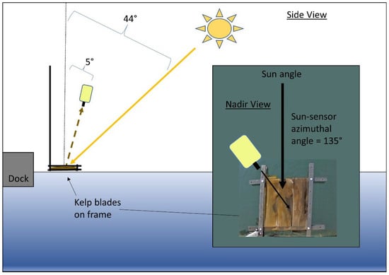
Figure 1.
Side view of submergence experiment showing the geometry of acquisition for spectroradiometer and angle of zenith for the sun. Inset shows nadir view of the experiment with the azimuthal angle between spectroradiometer and sun and kelp blades inside the black frame. Diagrams are not to scale.

Table 1.
Spectral parameters used to calculate above-water reflectance, as per Equation (1). All spectral measurements were collected using a calibrated ASD Fieldspec Handheld2 spectroradiometer with a one-degree fore optic (full viewing-angle), which detects a wavelength range from 325–1075 nm at 1 nm increments.
The solar elevation angle during the experiment was 46°, which ensured sun-glint did not contaminate the spectra based on our geometry of acquisition [33,34]. LT(λ) measurements were taken at 5° from a nadir viewing angle to avoid reflection of the white spectroradiometer in the field of view on the water surface, and a sensor-sun azimuthal angle of 135° was used to minimize specular reflection in the field of view (FOV) [33]. Lsky(λ) measurements were taken at 5° from zenith at the same azimuthal angle as LT(λ). The spectroradiometer was held one meter above water, giving a footprint ranging from about 1.6 cm at the surface to 3.8 cm when the target was 100 cm deep. This small footprint was meant to ensure that the LT(λ) measurements contained 100% kelp, avoiding mixed pixel considerations [35].
Here, was the proportionality factor of 0.0211, which relates the radiance measured directly from the sky to the estimated amount of sky radiance reflected off the sea surface based on wind, cloud cover, and geometry of acquisition [33]. (%) for kelp at the surface (0 cm) was not subjected to the sky glint correction. Hereafter, values for kelp on the surface, submerged kelp, and water with no kelp are referred to as R0+ for brevity.
The R0+ spectra were first smoothed using a mean filter with a window of 5 nm to reduce noise while maintaining spectral features, and all spectra were then manually inspected for quality control. All bulb spectra were highly consistent, however, some blade spectra showed deviations in both the blue-green and NIR regions; likely due to water movement between blades as kelp was submerged, causing opened gaps in the “canopy” of blades attached to the platform. These spectra likely did not contain 100% blades within the field of view and were therefore removed from further analysis (Table 2). Despite the removal of some blade spectra, the smallest sample size at any depth after quality control was at 90 cm with n = 10 spectral samples. Therefore, we do not expect that these removals biased the results of this study.
2.2. Simulation of Micasense and WorldView Band R0+ and Indices
After sky-glint correction, smoothing, and quality control of the spectra, R0+ measurements were simulated into bands of the WorldView-3 (R0+WV3) and the Micasense RedEdge-MX (R0+MSRE) sensors [36,37]. These sensors were chosen because both have a relatively high spatial resolution (WV3: 1.84 m; MSRE: ~1–10 cm), which is ideal for mapping kelp canopy in nearshore regions where it is likely to be submerged by tides and currents [16]. The R0+ at the bands of these sensors were simulated using Gaussian functions to estimate the sensor’s spectral response for each band, based on full-width half maximum values of each sensor’s band (Figure 2; Table 3). For a direct comparison, only the VNIR bands shared by both sensors were used for simulations.
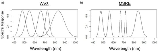
Figure 2.
Relative spectral responses at each band according to Gaussian functions were used to simulate the shared bands of (a) WorldView-3 (WV-3) earth observation satellite and (b) Micasense RedEdge-MX (MSRE) uncrewed aerial vehicle sensors—from left to right: blue, green, red, red-edge, and near-infrared band locations are shown.
2.3. Normalized Vegetation Indices
Once the hyperspectral data were simulated into the respective sensor bands, the R0+ at these bands were used to calculate normalized vegetation indices (VIn; Equation (2)), which are commonly used to enhance spectral features of interest and reduce sensitivity to environmental influences within remote sensing imagery [38,39]. We tested several band combinations for VIn as different band combinations may increase or decrease the separability between kelp and water in an image [40].
Because naming conventions for different VIn combinations are not ubiquitous across published literature, here, we referred to each VIn as the order in which bands appeared in the numerator of the VIn equation, separated by an underscore (Table 4).
One of the most commonly used VIn for kelp mapping is NIR_R, which was originally used to detect terrestrial vegetation because of the high NIR and low red signal [38], but has since been used for kelp canopy detection due to the similar spectral characteristics between kelp canopy and terrestrial vegetation [14]. More recently, NIR_R has been positively correlated with both the areal extent and biomass of kelp canopy [15,18,19]. However, various other combinations of visible and NIR bands have been used for kelp canopy detection with multispectral sensors. For instance, Schroeder et al. (2019b) used NIR_R and NIR_G for kelp detection with the WorldView-2 imagery. The NIR_G combination may be more accurate for detecting a wide range of chlorophyll levels [41] and has generally been found comparable with NIR_R in the detection of both floating and submerged vegetation [26]. Stekoll et al. (2006) found that NIR_B and NIR_G both provided higher kelp canopy and water separability in aerial imagery than NIR_R. Further, recent comparisons with multispectral UAV and satellite imagery have shown that RE indices can improve separability of Macrocystis canopy and water when compared with NIR based indices [17,42], although this improvement was not specifically attributed to improved detection of submerged portions of the kelp canopy in either study.
Here, we compared the statistical differences in NIR and RE-based VIn values. R0+MSRE and R0+WV3 bands were used to calculate NIR_B, NIR_G, NIR_R, and RE_B, RE_G, and RE_R for both bulb and blades separately, for each depth. The statistical analysis was comprised of (i) VIn values compared with one another at each depth from the surface to 100 cm, and (ii) VIn values for water (with no kelp) compared to one another. First, the dataset was tested for normality, and while quantile–quantile plots suggested reasonable normality of the data distributions, Levene’s test showed nearly all groupings for comparison displayed heterogeneity in variance. Therefore a non-parametric test was used in the analysis [43]. The Welch’s ANOVA test was used to determine whether significant differences between VIn existed at each depth, and the Games–Howell post hoc test was used to determine which indices were significantly different from one another [44,45]. As part of the analysis, we focused on the statistical results comparing the RE and NIR counterpart indices only (e.g., NIR_R & RE_R, or NIR_B & RE_B) at each depth.
2.4. Threshold Selection and Depth Limits for Kelp Detection
Once a VIn has been selected for classifying kelp in remote sensing imagery, a VIn value is then chosen as a threshold to classify the kelp and water within the imagery. For example, Cavanaugh et al. (2010) selected a threshold based on the 99.98th percentile highest NIR_R value from a histogram of known ‘deep water’ pixels, and Nijland et al. (2019) determined a NIR_R value of 0.05 to be a reasonable threshold by comparing pixel values of sparse kelp and open water. Since the R0+ values of water vary spatially and temporally according to optical constituents and inherent optical properties of water, as well as the characteristics of local substrate and bathymetry [28,46,47], these thresholds are often ‘dynamic’, and are therefore determined on an image-by-image basis. For satellite or airborne imagery covering a large regional scale, it may even be appropriate to select multiple thresholds across different regions within an image.
We determined a dynamic threshold for each VIn based on the maximum VIn value measured for water during the experiment following Cavanaugh et al. (2010). The depth where the mean VIn value of submerged kelp dropped below the dynamic threshold value was considered the depth where kelp was spectrally indistinguishable from water. Since our experiment was conducted under ideal conditions (flat calm water, full sun, etc.) the dynamic thresholds were all negative values and the maximum depth of detection using these thresholds likely overstate the potential depths for kelp detection in actual remote sensing imagery. Therefore, we also used a second VIn threshold of zero, based on the theoretical spectral properties of kelp within an individual pixel that contains 100% kelp. For example, within a pixel, if the R0+ value of band 2 (RE or NIR) equals the R0+ value as band 1 (the visible band), the numerator in the VIn equation (Equation (2)), and therefore the overall VIn value for that pixel, equals zero. This conservative threshold is closer to the values of 0.05 and 0.003 determined from remote sensing imagery by Nijland et al. (2019) and Mora-Soto et al. (2020), respectively.
Depth detection limits were reported to the nearest 10 cm depth on the shallow side of the threshold because the kelp was submerged in 10 cm intervals. To determine whether the detectable kelp (values above the threshold) and non-detectable kelp (values below the threshold) were statistically separable, the means for kelp measurements immediately above and below the threshold were compared for significant differences using Welch’s t-test [48].
3. Results
Here, we present the spectral characteristics of Nereocystis bulbs and blades as they are each submerged from the surface to 100 cm, as well as the changes seen in the hyperspectral data when they are simulated into multispectral sensor bandwidths. Next, we show VIn comparisons for kelp, focusing on comparing the RE and NIR counterpart indices (e.g., NIR_R & RE_R, or NIR_B & RE_B) at each depth, and finally, we present the depth detection limits for each VIn as determined by both dynamic and conservative thresholds.
3.1. Spectral Characteristics of Surface and Submerged Kelp
Overall, the R0+ of both Nereocystis bulbs and blades showed similar placement of spectral features, however, the magnitude of reflectance at these features was different (Figure 3a,b). For Nereocystis, spectral features in the visible wavelength ranges are largely due to absorption by a combination of chlorophyll-a, chlorophyll-c, and fucoxanthin pigments, which are characteristic pigments of bull kelp, as well as other kelp species [49,50]. Accordingly, here we saw a broad absorption feature in the 400–550 nm range and narrower absorption features around 633 and 675 nm for both bulbs and blades at the surface. These absorption features resulted in reflectance peaks at 575, 600, and 645 nm for both bulbs and blades (Figure 3a,b, insets). In the NIR region, broad reflectance peaks were detected from 690 nm (RE) to 900 nm (NIR) (Figure 3a,b, insets) and small, narrow peaks centered at 761 nm were observed (Figure 4a,b).
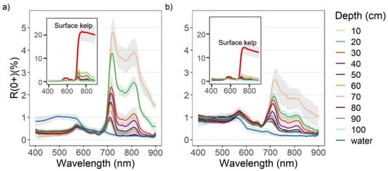
Figure 3.
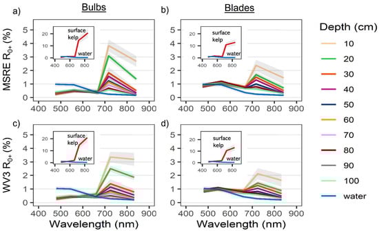
Reflectance values (R0+) between 400–900 nm (mean +/− sd) of water with (a) Nereocystis bulbs, and (b) Nereocystis blades, at incremental depths below water surface. The inset plots contain spectra of bulbs and blades on the surface compared to the same spectra of submerged bulb and blades as in the main plots, for the purpose of showing the difference in magnitude.
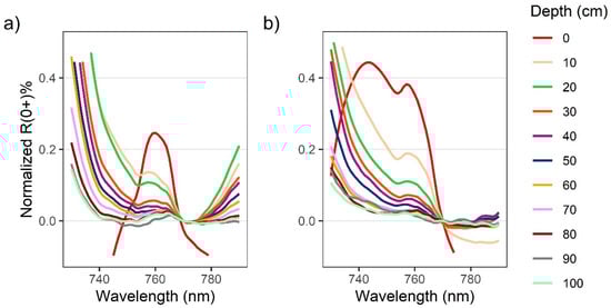
Figure 4.
Zoomed in plot showing solar-induced chlorophyll fluorescence (SICF) peaks centered at 761 nm for above-water R0+ for Nereocystis bulbs (a) and blades (b) at incremental depths below the water surface. Spectra are normalized at 770 nm to show relative changes to the shape of the SICF peak with submergence.
When kelp structures were submerged, the influence of the water and its constituents on the R0+ signal increased with submersion for both bulb and blades. The decreases in R0+ in the RE and NIR region were far greater than decreases in R0+ observed across the visible region of the spectra (Figure 3a,b, insets). With initial submersion below the water’s surface, the largest declines in the visible wavelength ranges were seen at 600 nm and 645 nm, although all peaks in the visible region continued to decrease with submersion (Figure 3a,b). While the R0+ at the absorption feature between 400–550 nm initially decreased with submersion, the reflectance then rose as the depth of submersion increased. In the NIR region of spectra for both structures, once kelp was submerged, the broad NIR peaks were replaced by two peaks centered around 715 nm and 815 nm (Figure 3a,b), hereafter referred to as the RE peak and the NIR peak, respectively. At each depth, the R0+ at the RE peak was higher than the NIR peak. As submergence increased, the position of the RE peak shifted toward lower wavelengths within the RE wavelength ranges while the position of the NIR peaks remained relatively stable. The small peaks at 761 nm remained stable, but decreased in magnitude with submersion, becoming difficult to visibly distinguish around 50 cm depth (Figure 4a,b).
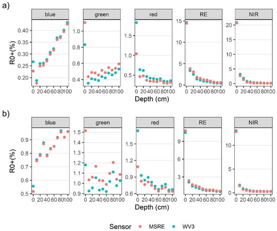
R0+WV and R0+MSRE showed the same general patterns as the hyperspectral data (Figure 5a–d). However, some spectral information was lost with the reduction of spectral resolution, such as the location and magnitude of different peaks. Overall, the differences in width and placement of bands resulted in only small differences in R0+WV3 and R0+MSRE band values (Figure A1a,b). For both bulbs and blades at the surface, differences in the visible wavelength ranges between R0+WV and R0+MSRE were less than 0.8% for the red, blue, and green bands, and these differences became even smaller as kelp was submerged. In the RE and NIR bands, differences between R0+WV and R0+MSRE were less than 0.3% on the surface. Once submerged to 10 cm, differences between R0+WV and R0+MSRE increased to 1.8% in the NIR bands and 0.5% in the RE bands, although similar to the visible bands, the differences between R0+WV and R0+MSRE also became smaller as the kelp was submerged deeper.
3.2. Vegetation Indices: Signal Strength and Depth-Detection Limits of Submerged Kelp
Generally, RE VIn values were higher than NIR VIn values at a given depth as kelp was submerged (Figure 6). For bulbs, RE VIn values decreased linearly from the surface to 100 cm, while NIR VIn showed a steeper linear decrease over the first 50 cm, followed by an inflection point and a lesser decline towards 100 cm. For blades, trendlines of both NIR and RE VIn resemble exponential functions, with the NIR VIn displaying a steeper decrease of values than the RE VIn.
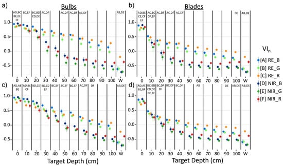
Figure 6.
Mean +/− sd of vegetation index (VIn) values for Nereocystis bulbs (a,c) and blades (b,d), submerged from the surface to 100 cm and water; derived from simulated Micasense RedEdge-MX (MSRE; a,b) and WorldView-3 (WV3; c,d) bandwidths. Paired letters above each column represent no significant differences (p ≥ 0.05) between mean index values at that depth.
Specifically, the Games–Howell post hoc tests showed that for kelp at the surface, RE VIn values were either smaller than or not significantly different from their counterpart NIR indices (Figure 6), depending on the visible band used. Once kelp was submerged, RE VIn values were significantly greater than their NIR counterparts at each depth with the MSRE sensor. However, with the WV3 sensor, RE VIn values were not significantly greater than their NIR counterparts until 10 cm and 20 cm depth for blades and bulbs, respectively. All VIn values for water were negative, meaning that the R0+ at the visible band used in the VIn was higher than the R0+ at the RE or NIR band used in the VIn, regardless of sensor simulation or index combination. RE_R consistently showed the highest values for water, followed by NIR_R, and there were no significant differences between RE_B and RE_G water values, nor for NIR_B and NIR_G water values. Here, we focused on the statistical results comparing the RE and NIR counterpart indices only (e.g., NIR_R & RE_R, or NIR_B & RE_B) at each depth, however, Figure 6 displays paired letters to indicate all pairs of VIn where no significant difference between VIn pairs was detected.
The depth detection limits varied based on sensor type, kelp structure, and thresholding method (Table 5; Figure 7). Overall, when using the conservative (more realistic) threshold of zero, RE VIn showed detection of kelp at least twice as deep as NIR VIn, and bulbs were detectable at greater depths than blades. Detection limits for the same VIn between sensors were generally within a range of 0–20 cm apart, although in a few cases (e.g., RE_R) these differences were larger. In addition, the choice of different visible bands for a VIn only resulted in detection limit differences up to 20 cm, with RE_R once again proving the exception. No RE indices crossed below the dynamic thresholds at 100 cm depth, meaning RE indices could detect kelp to at least 100 cm depth with these thresholds, while NIR indices could generally detect kelp to around 100 cm depth or less. In all cases, the RE indices at 100 cm depth were more separable from water than the NIR indices at the same depth. The use of different visible bands in the VIn combination generally resulted in detection limit differences of 0–30 cm for bulbs. For all measured depth detection limits, the index values measured at the increments 10 cm above and below the threshold remained divergent (p < 0.05), suggesting that all the measured results for conservative and dynamic thresholds are accurate to at least 10 cm increments.
Table 5.
Depth detection limits (cm) based on conservative threshold of 0.0 and the dynamic thresholds (maximum water value) for Nereocystis bulbs and blades, as simulated to Micasense RedEdge-MX (MSRE) and WorldView-3 (WV3) bandwidths.
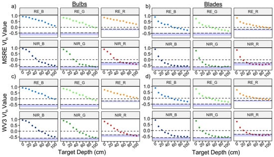
Figure 7.
Mean +/− sd of vegetation index (VIn) values for Nereocystis bulbs (a,c) and blades (b,d) submerged from the surface to 100 cm. derived from simulated Micasense RedEdge-MX (MSRE; a,b) and WorldView-3 (WV3; c,d) bandwidths. The black dashed lines at 0 represent the more conservative and realistic threshold, and the blue bars represent the full range of water values for each respective index, with the adjacent dashed lines representing the dynamic threshold.
4. Discussion
Overall, we found that submersion of kelp in water changes the shape and magnitude of R0+ in the RE and NIR region of kelp spectra (Figure 3), and Nereocystis bulbs had a higher magnitude R0+ in the RE and NIR region than blades (Figure 3). We also observed that RE VIn values for submerged kelp had higher separability from water than their NIR counterparts (Figure 6), meaning that kelp can be positively classified at deeper depths when using an RE VIn (Table 3; Figure 7). Our results also showed that VIn that used a visible band with high R0+ (e.g., green or blue) had worse detectability for submerged kelp than a VIn that used a visible band with low R0+ (e.g., red). Together, these findings have important implications for the application of kelp remote sensing to the applied monitoring of kelp forests.
4.1. Spectral Characteristics of Kelp as It Is Submerged
A broad R0+ peak across the NIR region was observed for surface measurements of Nereocystis as a result of the interaction of light with the cellular structure of the kelp [51]. Once submerged, our experiment showed two key changes in the NIR region of the kelp spectra (Figure 3), both due to characteristic absorption features of water: (1) the splitting of the single broad NIR peak into two narrower RE and NIR peaks due to prominent water absorption feature at 760 nm [52] and (2) higher R0+ at the RE peak versus the NIR peak, resulting from the continually increasing absorption of light by water above 600 nm [22]. Since Macrocystis and Nereocystis are spectrally similar to one another in the NIR region [15,18,27,50], and the changes seen in the spectra of submerged kelp are due to properties of water absorption, we expect that the spectral results of this experiment are generally applicable to both Macrocystis and Nereocystis canopies, making these findings relevant for surface-canopy forming kelp species globally.
The results of these experiments were generally in line with our expectations according to similar studies of submerged aquatic vegetation [24,25], although there were some interesting phenomena seen in the spectra that are worth noting. In the visible region of the spectra, R0+ in the red wavelength range decreased with depth, as expected. However, the R0+ at the absorption feature between 400 and 550 nm increased slightly with submersion. We hypothesize that this increase in R0+ is due to the scattering of light by the conditions of the water optical constituents, thus increasing the R0+ with depth. As such, we suspect that this increase in R0+ may be specific to the water conditions during the experiment and may not have occurred if the water had contained more optical constituents that absorb blue light, such as colored dissolved organic matter. Another interesting phenomenon noted in the floating kelp spectra was what appeared to be a sunlight-induced chlorophyll fluorescence (SICF) peak at 761 nm (Figure 4). Within the NIR region, photosynthetic organisms generally have a broad SICF peak centered at 740 nm [53]. However, due to the high magnitude of the NIR reflectance, the SICF is usually only visible as a small, narrow peak centered at 761 nm. Typically, the R0+ within the NIR wavelength range overwhelms the signal from SICF, however, atmospheric gasses highly absorb incoming irradiance at 761 nm, which can create a fill-in effect by the SICF in this region [53]. While this phenomenon has been correlated with photosynthetic output and general health of terrestrial vegetation and phytoplankton [53,54], we are not aware of any publications that report an SICF peak in kelp spectra, and this may present an opportunity for future hyperspectral research. Once kelp was submerged the SICF feature was dampened, and therefore future research should take note of the amount of kelp at the surface if attempting to derive information from an SICF peak.
4.2. NIR Differences between Nereocystis Bulbs and Blades
The magnitude of reflectance across the NIR region in vegetation is generally due to the cellular structure of the respective tissues [55]. Both Nereocystis bulb and blade tissues are composed of the same three cellular layers: the meristoderm, the medulla, and the cortex. The meristoderm is a thin chloroplast-packed epidermal layer that surrounds the entire individual [56], and the medulla is a complex web of filaments that acts as a transportation system within the kelp, composing the innermost layer of kelp tissue [57,58]. Between these two layers is the cortex, which connects the meristoderm to the medulla, and generally provides structural support for the kelp [56,59]. Given this structural arrangement, we speculate that the NIR signal from bulbs is consistently higher compared to the blades’ signal because (1) the bulb cortex is many times thicker than the blade cortex [57,59]; and (2) the gas cavity of the bulb is lined by the medulla [57], creating a high surface area with many large refractive differences—similar to the mesophyll layer of a terrestrial leaf [55,60]. In comparison, the blade medulla is housed in a gelatinous extracellular matrix between cells [57], and with no gas cavities, the refractive differences are much smaller, allowing for increased transmittance of NIR light through the blades [55]. For our experiment, spectral measurements for blades were taken using a single blade wrapped around the polyethylene frame with only slight overlap between the edges of the blade. However, Nereocystis individuals may have between 30–60 blades each. Overall, a thicker mass of blade tissues due to high overlap may result in higher R0+ in the RE and NIR wavelength ranges than seen in this experiment.
4.3. The Implications of VIn Saturation for Detection of Floating and Submerged Kelp
When the density or biomass of the vegetation increases within a pixel of remote sensing imagery, the VIn for that pixel will asymptotically approach a saturation (i.e., a high VIn value) [39,61]. This happens because when vegetation is dense, the R0+ at band 2 (NIR or RE) is large relative to the R0+ at band 1 (the visible band). Our spectral measurements contained 100% kelp within the field of view, and accordingly, the VIn values calculated from the multispectral simulations were saturated when kelp was at the surface. Therefore, it is critical to understand how saturation affected the VIn values of floating kelp, as well as when kelp was submerged. For example, our WV3 simulations for bulbs at the surface showed that the R0+ at NIR and RE bands were large compared to the red band (21%, 14%, and 1%, respectively). As such, both NIR_R and RE_R indices for bulbs at the surface were approaching saturation (0.83 and 0.77 respectively) and either index would perform relatively well for detecting floating kelp if a VIn of zero was used as a threshold to classify kelp and water. When the bulb was submerged, the R0+ in the NIR and RE bands decreased rapidly by 10 cm depth (3.2 and 3.4% respectively) but were still relatively high compared to the red band, which had also decreased (0.6%), and therefore the NIR_R and RE_R values (0.66 and 0.68 respectively) were still relatively saturated, despite the large decreases in R0+ at the RE and NIR bands (Figure 5). As the kelp continued to be submerged, the R0+ at the NIR, RE, and red bands all continued to decrease, however, the R0+ at the NIR band decreased at a faster rate and therefore the NIR_R value dropped below the threshold of zero by 50 cm while the RE_R value was still above the threshold by 100 cm. Ultimately, this example shows that due to VIn saturation, the choice of RE or NIR will make little to no difference in classification of kelp at or near the surface. However, once submerged, the use of an RE VIn will still detect kelp deeper than an NIR VIn.
4.4. Depth Detection Limits and Separability between Kelp and Water
While it is important to understand how VIn values change as kelp is submerged, ultimately the accuracy of submerged kelp classification depends on the spectral separability between the submerged kelp and water. Here, we defined the depth at which kelp and water were no longer separable as the depth at where VIn values for submerged kelp decreased below the threshold value. RE VIn values for kelp and water had higher separability at deeper depths than their NIR counterparts (Figure 6), meaning that deeper kelp can be accurately classified when using an RE VIn. Higher separability between kelp and water classes when using RE VIn has been documented using both high spatial-resolution multispectral UAV imagery [13] and with moderate spatial-resolution multispectral satellite imagery of Macrocystis [42], indicating that slight submergence of kelp surface-canopy may play a larger role in detection than previously thought.
While the choice between RE and NIR VIn was an important factor in submerged kelp detection, the choice of the visible band can also shift the detection limits of submerged kelp. Our results show that both the water and submerged kelp spectra had higher R0+ in the green and blue wavelength ranges than in the red, and as such, submerged kelp became undetectable at shallower depths when using NIR_R compared to NIR_G or NIR_B. In the visible wavelength ranges, red is absorbed fastest by the water column, and in our experiment, the NIR signal is generally absorbed by around 50 cm depth, making it reasonable for this pairing to consistently have the shallowest detection limits for submerged kelp. At depths where the RE or NIR signal of kelp can no longer be detected, Figure 7 shows that subtle differences between kelp and water in the blue and green bands can still result in the kelp signal remaining above the dynamic threshold. However, these differences are small, and because conditions during the experiment were controlled, the added spectral noise from in situ environmental factors would likely complicate the detection of both surface and submerged kelp in more realistic situations. For example, the blue wavelength ranges can be highly compromised in remote sensing imagery [29,46], with local variation in atmospheric composition reducing the certainty of accuracy for blue band values. Additionally, the optical constituents of coastal water can be highly spatiotemporally variable—affecting all regions of the spectra [28,46]. At high concentrations phytoplankton in the water column may result in changes to reflectance in the visible wavelength ranges as well as high RE or NIR reflectance [62], while changes to optical constituents such as sediment or CDOM may also impede the detection of submerged kelp [47,63].
In this experiment, the optical water conditions (Secchi = 7.5) were typical of the coastal waters of British Columbia [18,28,64]. Considering the Secchi measurement, the local depth (12 m), and the R0+ from water with no kelp (Figure 3), the bottom substrate signal was not part of the measured R0+ in our experiment. Yet kelp on the coast of British Columbia is often found as fringing canopies near the shoreline [18], which can result in a strong contribution of benthic substrate to the R0+ measured by space and air-borne platforms. Reflectance from shallow benthic features can result in highly variable R0+ in both the visible and near-infrared wavelength ranges, resulting in misclassification of submerged vegetation as canopy kelp [47,64]. Therefore, it is important to understand site characteristics (e.g., bathymetry and water turbidity) to define better the use of NIR or RE for kelp classification. For instance, if enough understanding of the local conditions at the time of imagery acquisition is not available, it may be more appropriate to use NIR_R to reduce the addition of signal of the bottom substrate. Alternately, if imagery or associated ground truth data have a high enough spatial resolution (e.g., from UAV or other aerial platforms), visual interpretation of surface-canopy morphology from expert knowledge may be adequate for manual classification or ground truthing when using an RE VIn.
4.5. Implications for Mixed Pixels
During the experiment, spectral data were collected using a small footprint to reduce uncertainties associated with having the reflectance signal of multiple targets within the field of view (i.e., mixed pixels). However, remote sensing imagery often contains mixed pixels [16,35]. This becomes especially problematic when sensors have a lower spatial resolution, where erroneous classification of a pixel as kelp may result in the overestimation of total kelp canopy. Multiple end-member spectral mixture analysis (MESMA) is an approach that has been applied to satellite imagery for both Macrocystis [11,35] and Nereocystis canopy [19,65] to determine what proportion of the pixel is kelp, and what proportion is water. When MESMA is applied to remote sensing imagery for kelp detection, it is assumed that all VIn or band values within a pixel are a linear combination of kelp and water end-members [35]. However, if the kelp fraction within a pixel is low enough, the spectral contribution from water may overwhelm the kelp signal, lowering the overall pixel value and allowing the pixel to be erroneously classified as water [19,27]. Our results suggest that if submerged kelp is present when MESMA is performed, which is most often the case, the reduced signal from the submerged kelp within the pixel may lead to an underestimation of the kelp fraction within the pixel. Using an RE VIn when performing MESMA may allow the user to detect more submerged kelp, thus contributing to a higher overall pixel value and increasing the accuracy of the classification. This may be especially relevant if attempting to determine relationships between remote sensing imagery and biomass, since Nereocystis blades show a higher correlation to the mass of the individual than any other metric tested [10]. Further, Nereocystis canopy generally has less dense biomass at the surface than Macrocystis [65,66], and, therefore, is more likely to be misclassified in moderate or low spatial resolution imagery.
5. Conclusions
Our experiment contributes new, detailed information on the effects of kelp submersion on the above water reflectance, as well as a comparison of the depth detection limits of kelp when using red-edge and near-infrared indices. We determined that the near-infrared region of kelp spectra is strongly absorbed upon submersion, however, there is a narrow spectral peak in the red-edge region that can be used to enhance the remote sensor’s ability to detect submerged kelp due to lower water absorption. Detection limits varied based on kelp tissue, the thresholding method, and the visible band used in the vegetation index calculation, but overall, red-edge vegetation indices detected deeper than their counterpart NIR indices, which may allow the remote sensor to improve accuracy when mapping sparse and partially submerged kelp canopy or attempting to derive biomass from canopy reflectance values. Kelp forests may be mapped using remote sensing for various reasons, ranging from estimation of biomass for kelp harvesting to multi-year temporal analyses to assess the impacts of environmental drivers on kelp ecosystems. Yet kelp systems can be highly variable in abundance between years, and our study shows that the spectral variables used to detect kelp canopy in remote sensing imagery play an important role in the amount of submerged kelp canopy detected. Therefore, it is critical for a remote sensing user to understand how the physical interaction between light and water may affect the depth at which kelp can be detected. For example, RE VIn might be especially useful if resource managers are attempting to set quotas for harvestable biomass of Nereocystis and wish to detect as much blade biomass as possible for specific beds. However, if one wishes to reduce detection of subsurface kelp canopy or other shallow benthic vegetation, we recommend the use of the NIR_R (NDVI), which consistently had the shallowest detection limits of the indices tested.
Author Contributions
B.T., M.C. and L.Y.R. designed the study. B.T. and L.Y.R. carried out the experiment. B.T. conducted the analysis and wrote the manuscript with input and guidance from M.C., L.Y.R., F.J. and M.H.-L. All authors have read and agreed to the published version of the manuscript.
Funding
During this research BT was supported through a MITACS Accelerate internship with the Hakai Institute, as well as an NSERC CGS-M award and Costa’s NSERC-DG.
Institutional Review Board Statement
Not applicable.
Informed Consent Statement
Not applicable.
Data Availability Statement
Data are available for research purposes upon request to the authors’ institutions.
Acknowledgments
We thank the Hakai Institute and the Canada NSERC-DG for providing funding for this research as well as Robert Atwood for letting us use his slip at the Oak Bay marina to test this experiment. Also, thank you to Lianna Gendall for helping with the kelp in the graphical abstract.
Conflicts of Interest
The authors declare no conflict of interest.
References
- Druehl, L.D.; Wheeler, W.N. Population Biology of Macrocystis Integrifolia from British Columbia, Canada. Mar. Biol. 1986, 90, 173–179. [Google Scholar] [CrossRef]
- Kain, J.M. Patterns of Relative Growth in Nereocystis Luetkeana (Phaeophyta). J. Phycol. 1987, 23, 181–187. [Google Scholar] [CrossRef]
- Krumhansl, K.A.; Okamoto, D.K.; Rassweiler, A.; Novak, M.; Bolton, J.J.; Cavanaugh, K.C.; Connell, S.D.; Johnson, C.R.; Konar, B.; Ling, S.D.; et al. Global Patterns of Kelp Forest Change over the Past Half-Century. Proc. Natl. Acad. Sci. USA 2016, 113, 13785–13790. [Google Scholar] [CrossRef] [PubMed] [Green Version]
- Druehl, L.D. The Pattern of Laminariales Distribution in the Northeast Pacific. Phycologia 1970, 9, 237–247. [Google Scholar] [CrossRef]
- Jackson, G.A. Internal Wave Attenuation by Coastal Kelp Stands. J. Phys. Oceanogr. 1984, 14, 1300–1306. [Google Scholar] [CrossRef] [Green Version]
- Mork, M. The Effect of Kelp in Wave Damping. Sarsia 1996, 80, 323–327. [Google Scholar] [CrossRef]
- Krumhansl, K.A.; Scheibling, R. Production and Fate of Kelp Detritus. Mar. Ecol. Prog. Ser. 2012, 467, 281–302. [Google Scholar] [CrossRef] [Green Version]
- Olson, A.M.; Hessing-Lewis, M.; Haggarty, D.; Juanes, F. Nearshore Seascape Connectivity Enhances Seagrass Meadow Nursery Function. Ecol. Appl. 2019, 29, e01897. [Google Scholar] [CrossRef]
- Springer, Y.; Hays, C.; Carr, M.H.; Mackey, M. Ecology and Management of the Bull Kelp, Nereocystis Luetkeana: A Synthesis with Recommendations for Future Research; Lenfest Ocean Program: Washington, DC, USA, 2007; pp. 1–53. [Google Scholar]
- Stekoll, M.S.; Deysher, L.E.; Hess, M. A Remote Sensing Approach to Estimating Harvestable Kelp Biomass. J. Appl. Phycol. 2006, 18, 323–334. [Google Scholar] [CrossRef]
- Bell, T.W.; Allen, J.G.; Cavanaugh, K.C.; Siegel, D.A. Three Decades of Variability in California’s Giant Kelp Forests from the Landsat Satellites. Remote Sens. Environ. 2020, 238, 110811. [Google Scholar] [CrossRef]
- Pfister, C.A.; Berry, H.D.; Mumford, T. The Dynamics of Kelp Forests in the Northeast Pacific Ocean and the Relationship with Environmental Drivers. J. Ecol. 2017, 106, 1520–1533. [Google Scholar] [CrossRef]
- Cavanaugh, K.C.; Bell, T.; Costa, M.; Eddy, N.E.; Gendall, L.; Gleason, M.G.; Hessing-Lewis, M.; Martone, R.; McPherson, M.; Pontier, O.; et al. A Review of the Opportunities and Challenges for Using Remote Sensing for Management of Surface-Canopy Forming Kelps. Front. Mar. Sci. 2021, 8, 1536. [Google Scholar] [CrossRef]
- Jensen, J.R. Remote Sensing Techniques for Kelp Surveys. Photogramm. Eng. Remote Sens. 1980, 46, 743–755. [Google Scholar]
- Cavanaugh, K.; Siegel, D.; Kinlan, B.; Reed, D. Scaling Giant Kelp Field Measurements to Regional Scales Using Satellite Observations. Mar. Ecol. Prog. Ser. 2010, 403, 13–27. [Google Scholar] [CrossRef] [Green Version]
- Schroeder, S.B.; Dupont, C.; Boyer, L.; Juanes, F.; Costa, M. Passive Remote Sensing Technology for Mapping Bull Kelp (Nereocystis Luetkeana): A Review of Techniques and Regional Case Study. Glob. Ecol. Conserv. 2019, 19, e00683. [Google Scholar] [CrossRef]
- Cavanaugh, K.C.; Cavanaugh, K.C.; Bell, T.W.; Hockridge, E.G. An Automated Method for Mapping Giant Kelp Canopy Dynamics from UAV. Front. Environ. Sci. 2021, 8, 587354. [Google Scholar] [CrossRef]
- Schroeder, S.B.; Boyer, L.; Juanes, F.; Costa, M. Spatial and Temporal Persistence of Nearshore Kelp Beds on the West Coast of British Columbia, Canada Using Satellite Remote Sensing. Remote Sens. Ecol. Conserv. 2019, 6, 327–343. [Google Scholar] [CrossRef] [Green Version]
- Hamilton, S.L.; Bell, T.W.; Watson, J.R.; Grorud-Colvert, K.A.; Menge, B.A. Remote Sensing: Generation of Long-Term Kelp Bed Data Sets for Evaluation of Impacts of Climatic Variation. Ecology 2020, 101, e03031. [Google Scholar] [CrossRef]
- Britton-Simmons, K.; Eckman, J.E.; Duggins, D.O. Effect of Tidal Currents and Tidal Stage on Estimates of Bed Size in the Kelp Nereocystis Luetkeana. Mar. Ecol. Prog. Ser. 2008, 355, 95–105. [Google Scholar] [CrossRef] [Green Version]
- Filella, I.; Penuelas, J. The Red Edge Position and Shape as Indicators of Plant Chlorophyll Content, Biomass and Hydric Status. Int. J. Remote Sens. 1994, 15, 1459–1470. [Google Scholar] [CrossRef]
- Pegau, W.S.; Gray, D.; Zaneveld, J.R.V. Absorption and Attenuation of Visible and Near-Infrared Light in Water: Dependence on Temperature and Salinity. Appl. Opt. 1997, 36, 6035–6046. [Google Scholar] [CrossRef] [PubMed] [Green Version]
- Han, L.; Rundquist, D.C. The Spectral Responses of Ceratophyllum Demersum at Varying Depths in an Experimental Tank. Int. J. Remote Sens. 2003, 24, 859–864. [Google Scholar] [CrossRef]
- Kearney, M.S.; Stutzer, D.; Turpie, K.; Stevenson, J.C. The Effects of Tidal Inundation on the Reflectance Characteristics of Coastal Marsh Vegetation. J. Coast. Res. 2009, 256, 1177–1186. [Google Scholar] [CrossRef]
- Turpie, K.R. Explaining the Spectral Red-Edge Features of Inundated Marsh Vegetation. J. Coast. Res. 2013, 290, 1111–1117. [Google Scholar] [CrossRef]
- Song, B.; Park, K. Detection of Aquatic Plants Using Multispectral UAV Imagery and Vegetation Index. Remote Sens. 2020, 12, 387. [Google Scholar] [CrossRef] [Green Version]
- Nijland, W.; Reshitnyk, L.; Rubidge, E. Satellite Remote Sensing of Canopy-Forming Kelp on a Complex Coastline: A Novel Procedure Using the Landsat Image Archive. Remote Sens. Environ. 2019, 220, 41–50. [Google Scholar] [CrossRef]
- Phillips, S.R.; Costa, M. Spatial-Temporal Bio-Optical Classification of Dynamic Semi-Estuarine Waters in Western North America. Estuar. Coast. Shelf Sci. 2017, 199, 35–48. [Google Scholar] [CrossRef]
- Mobley, C.D. Light and Water: Radiative Transfer in Natural Waters; Academic Press: San Diego, CA, USA, 1994; ISBN 978-0-12-502750-2. [Google Scholar]
- Dierssen, H.M.; Chlus, A.; Russell, B. Hyperspectral Discrimination of Floating Mats of Seagrass Wrack and the Macroalgae Sargassum in Coastal Waters of Greater Florida Bay Using Airborne Remote Sensing. Remote Sens. Environ. 2015, 167, 247–258. [Google Scholar] [CrossRef]
- Hu, L.; Hu, C.; Ming-Xia, H. Remote Estimation of Biomass of Ulva Prolifera Macroalgae in the Yellow Sea. Remote Sens. Environ. 2017, 192, 217–227. [Google Scholar] [CrossRef]
- ASD Inc. ASD Light Theory and Measurement Using the FieldSpec HandHeld 2 Portable Spectroradiometer; ASD Inc.: Longmont, CO, USA, 2017. [Google Scholar]
- Mobley, C.D. Estimation of the Remote-Sensing Reflectance from above-Surface Measurements. Appl. Opt. 1999, 38, 7442–7455. [Google Scholar] [CrossRef]
- Mount, R. Acquisition of Through-Water Aerial Survey Images. Available online: https://www.ingentaconnect.com/content/asprs/pers/2005/00000071/00000012/art00005 (accessed on 8 April 2020).
- Cavanaugh, K.; Siegel, D.; Reed, D.; Dennison, P. Environmental Controls of Giant-Kelp Biomass in the Santa Barbara Channel, California. Mar. Ecol. Prog. Ser. 2011, 429, 1–17. [Google Scholar] [CrossRef] [Green Version]
- Micasense RedEdge-MX—MicaSense. Available online: https://micasense.com/rededge-mx/ (accessed on 17 January 2022).
- Maxar WorldView-3. Available online: https://resources.maxar.com/data-sheets/worldview-3 (accessed on 17 January 2022).
- Rouse, W.; Haas, R.H.; Deering, W. Monitoring the Vernal Advancement and Retrogradation (Green Wave Effect) of Natural Vegetation; Goddard Space Flight Center: Greenbelt, MD, USA, 1974; p. 87.
- Tucker, C.J. Red and Photographic Infrared Linear Combinations for Monitoring Vegetation. Remote Sens. Environ. 1979, 8, 127–150. [Google Scholar] [CrossRef] [Green Version]
- Augenstein, E.W.; Stow, D.; Hope, A. Evaluation of SPOT HRV-XS Data for Kelp Resource Inventories. Photogramm. Eng. Remote Sens. 1991, 57, 501–509. [Google Scholar]
- Gitelson, A.A.; Kaufman, Y.J.; Merzlyak, M.N. Use of a Green Channel in Remote Sensing of Global Vegetation from EOS-MODIS. Remote Sens. Environ. 1996, 58, 289–298. [Google Scholar] [CrossRef]
- Mora-Soto, A.; Palacios, M.; Macaya, E.C.; Gómez, I.; Huovinen, P.; Pérez-Matus, A.; Young, M.; Golding, N.; Toro, M.; Yaqub, M.; et al. A High-Resolution Global Map of Giant Kelp (Macrocystis Pyrifera) Forests and Intertidal Green Algae (Ulvophyceae) with Sentinel-2 Imagery. Remote Sens. 2020, 12, 694. [Google Scholar] [CrossRef] [Green Version]
- Schultz, B.B. Levene’s Test for Relative Variation. Syst. Biol. 1985, 34, 449–456. [Google Scholar] [CrossRef]
- Algina, J.; Oshima, T.C.; Lin, W.-Y. Type I Error Rates for Welch’s Test and James’s Second-Order Test Under Nonnormality and Inequality of Variance When There Are Two Groups. J. Educ. Stat. 1994, 19, 275–291. [Google Scholar] [CrossRef] [Green Version]
- Shingala, M.C.; Rajyaguru, D.A. Comparison of Post Hoc Tests for Unequal Variance. Int. J. New Technol. Sci. Eng. 2015, 2, 12. [Google Scholar]
- Morel, A.; Prieur, L. Analysis of Variations in Ocean Color. Limnol. Oceanogr. 1977, 22, 709–722. [Google Scholar] [CrossRef]
- Vahtmäe, E.; Paavel, B.; Kutser, T. How Much Benthic Information Can Be Retrieved with Hyperspectral Sensor from the Optically Complex Coastal Waters? J. Appl. Remote Sens. 2020, 14, 016504. [Google Scholar] [CrossRef]
- Welch, B.L. The Generalization of ‘Student’s’ Problem When Several Different Population Variances Are Involved. Biometrika 1947, 34, 28–35. [Google Scholar] [CrossRef]
- Wheeler, W.N.; Smith, R.G.; Srivastava, L.M. Seasonal Photosynthetic Performance of Nereocystis Luetkeana. Can. J. Bot. 1984, 62, 664–670. [Google Scholar] [CrossRef]
- Olmedo-Masat, O.M.; Raffo, M.P.; Rodríguez-Pérez, D.; Arijón, M.; Sánchez-Carnero, N. How Far Can We Classify Macroalgae Remotely? An Example Using a New Spectral Library of Species from the South West Atlantic (Argentine Patagonia). Remote Sens. 2020, 12, 3870. [Google Scholar] [CrossRef]
- Liew, O.W.; Chong, P.C.J.; Li, B.; Asundi, A.K. Signature Optical Cues: Emerging Technologies for Monitoring Plant Health. Sensors 2008, 8, 3205–3239. [Google Scholar] [CrossRef] [PubMed] [Green Version]
- Ruru, D.; Yingqing, H.; Yan, Q.; Qidong, C.; Lei, C. Measuring Pure Water Absorption Coefficient in the Near-Infrared. J. Remote Sens. 2012, 16, 192–206. [Google Scholar]
- Meroni, M.; Rossini, M.; Guanter, L.; Alonso, L.; Rascher, U.; Colombo, R.; Moreno, J. Remote Sensing of Solar-Induced Chlorophyll Fluorescence: Review of Methods and Applications. Remote Sens. Environ. 2009, 113, 2037–2051. [Google Scholar] [CrossRef]
- Lu, Y.; Li, L.; Hu, C.; Li, L.; Zhang, M.; Sun, S.; Lv, C. Sunlight Induced Chlorophyll Fluorescence in the Near-Infrared Spectral Region in Natural Waters: Interpretation of the Narrow Reflectance Peak around 761 Nm. J. Geophys. Res. Ocean. 2016, 121, 5017–5029. [Google Scholar] [CrossRef] [Green Version]
- Knipling, E.B. Physical and Physiological Basis for the Reflectance of Visible and Near-Infrared Radiation from Vegetation. Remote Sens. Environ. 1970, 1, 155–159. [Google Scholar] [CrossRef]
- Nicholson, N.L. Field Studies on the Giant Kelp. Nereocystis. J. Phycol. 1970, 6, 177–182. [Google Scholar] [CrossRef]
- Nicholson, N.L. Anatomy of the Medulla of Nereocystis. Bot. Mar. 1976, 19, 23–31. [Google Scholar] [CrossRef]
- Schmitz, K.; Srivastava, L.M. The Fine Structure of Sieve Elements of Nereocystis Lütkeana. Am. J. Bot. 1976, 63, 679–693. [Google Scholar] [CrossRef]
- Nicholson, N.L.; Briggs, W.R. Translocation of Photosynthate in the Brown Alga Nereocystis. Am. J. Bot. 1972, 59, 97–106. [Google Scholar] [CrossRef]
- Slaton, M.R.; Hunt, E.R.; Smith, W.K. Estimating Near-Infrared Leaf Reflectance from Leaf Structural Characteristics. Am. J. Bot. 2001, 88, 278–284. [Google Scholar] [CrossRef] [PubMed]
- Mutanga, O.; Skidmore, A.K. Hyperspectral Band Depth Analysis for a Better Estimation of Grass Biomass (Cenchrus Ciliaris) Measured under Controlled Laboratory Conditions. Int. J. Appl. Earth Obs. Geoinf. 2004, 5, 87–96. [Google Scholar] [CrossRef]
- Gower, J.F.R.; Doerffer, R.; Borstad, G.A. Interpretation of the 685nm Peak in Water-Leaving Radiance Spectra in Terms of Fluorescence, Absorption and Scattering, and Its Observation by MERIS. Int. J. Remote Sens. 1999, 20, 1771–1786. [Google Scholar] [CrossRef]
- O’Neill, J.D.; Costa, M.; Sharma, T. Remote Sensing of Shallow Coastal Benthic Substrates: In Situ Spectra and Mapping of Eelgrass (Zostera Marina) in the Gulf Islands National Park Reserve of Canada. Remote Sens. 2011, 3, 975–1005. [Google Scholar] [CrossRef] [Green Version]
- O’Neill, J.D.; Costa, M. Mapping Eelgrass (Zostera Marina) in the Gulf Islands National Park Reserve of Canada Using High Spatial Resolution Satellite and Airborne Imagery. Remote Sens. Environ. 2013, 133, 152–167. [Google Scholar] [CrossRef]
- Finger, D.J.I.; McPherson, M.L.; Houskeeper, H.F.; Kudela, R.M. Mapping Bull Kelp Canopy in Northern California Using Landsat to Enable Long-Term Monitoring. Remote Sens. Environ. 2021, 254, 112243. [Google Scholar] [CrossRef]
- Sutherland, I.R. Kelp Inventory, 1989 The Vancouver Island and Malcolm Island Shores of Queen Charlotte Strait Including a Summary of Historical Inventory Information for the Area; Kelp Inventory; Ministry of Environment: Vancouver, BC, Canada, 1990; p. 46.
Publisher’s Note: MDPI stays neutral with regard to jurisdictional claims in published maps and institutional affiliations. |
© 2022 by the authors. Licensee MDPI, Basel, Switzerland. This article is an open access article distributed under the terms and conditions of the Creative Commons Attribution (CC BY) license (https://creativecommons.org/licenses/by/4.0/).