Abstract
Airborne laser scanning (ALS) is increasingly used for detailed vegetation structure mapping; however, there are many local-scale applications where it is economically ineffective or unfeasible from the temporal perspective. Unmanned aerial vehicles (UAVs) or airborne imagery (AImg) appear to be promising alternatives, but only a few studies have examined this assumption outside economically exploited areas (forests, orchards, etc.). The main aim of this study was to compare the usability of normalized digital surface models (nDSMs) photogrammetrically derived from UAV-borne and airborne imagery to those derived from low- (1–2 pts/m2) and high-density (ca. 20 pts/m2) ALS-scanning for the precise local-scale modelling of woody vegetation structures (the number and height of trees/shrubs) across six dynamically changing shrubland sites. The success of the detection of woody plant tops was initially almost 100% for UAV-based models; however, deeper analysis revealed that this was due to the fact that omission and commission errors were approximately equal and the real accuracy was approx. 70% for UAV-based models compared to 95.8% for the high-density ALS model. The percentage mean absolute errors (%MAE) of shrub/tree heights derived from UAV data ranged between 12.2 and 23.7%, and AImg height accuracy was relatively lower (%MAE: 21.4–47.4). Combining UAV-borne or AImg-based digital surface models (DSM) with ALS-based digital terrain models (DTMs) significantly improved the nDSM height accuracy (%MAE: 9.4–13.5 and 12.2–25.0, respectively) but failed to significantly improve the detection of the number of individual shrubs/trees. The height accuracy and detection success using low- or high-density ALS did not differ. Therefore, we conclude that UAV-borne imagery has the potential to replace custom ALS in specific local-scale applications, especially at dynamically changing sites where repeated ALS is costly, and the combination of such data with (albeit outdated and sparse) ALS-based digital terrain models can further improve the success of the use of such data.
1. Introduction
Accurate information about woody vegetation structure characteristics (height, crown diameter, number of individuals, species, biomass estimation, landscape patterns, etc.) is very important for tasks associated with nature conservation and management [1] and is beneficial for other analyses of applied ecology for evaluating biodiversity, e.g., [2,3,4], forest species composition [5], carbon storage dynamics [6], pest outbreaks [7], forest microclimates [8], canopy gap patterns [9], and biomass volumes [10]. While describing forest structures is more or less standardized, it remains difficult in specific shrubland ecosystems with dynamically changing sparse woody vegetation, the high nature conservation value (i.e., high diversity of habitats and, in effect, high biodiversity) of which is associated with frequent landscape disturbances caused by the presence of military activities [11] or fires [12], among others. Such disturbances usually have positive effects on biodiversity [13,14] and cause changes in vegetation composition (especially lower trees and shrubs). The monitoring of such changes with field surveys is time-consuming and difficult; hence, a time-effective solution for the mapping of such areas at reasonable costs is needed for not only ecological studies but also forestry and nature conservation management purposes.
Field surveys of the woody plant structure characteristics are usually time-consuming, especially in highly heterogeneous “close-to-nature” environments. Remote sensing (RS) methods using airborne laser scanning (ALS; also known as airborne light detection and ranging/lidar) are, thanks to their proven advantages, becoming popular and beneficial in detailed mapping of natural environments including shrubland sites with sparse woody vegetation [15]. Therefore, ALS can nowadays be considered to represent an appropriate data source for describing woody vegetation structures in detail [16]. However, there are many local-scale applications where ALS is ineffective from the economical or temporal perspectives (the custom airborne laser scanning of small areas would be costly and associated with long wait times for the availability of ALS providers). For such applications, unmanned aerial vehicle (UAV) or airborne imagery (AImg) processed through image-matching techniques (such as structure from motion) seem to be promising alternatives that may be beneficial for the detailed mapping of vegetation at local scales [17]; there are, however, still not enough studies proving this in specific environments. Comprehensive reviews of both ALS and image-based techniques have been presented, e.g., by White et al. [18] and Puliti et al. [19].
A vegetation structure consists of horizontal and vertical components. The horizontal component describes the landscape structure, while the vertical component represents the configuration of aboveground vegetation [20]. The calculation of woody vegetation structure characteristics (especially those describing vertical structure) typically requires a normalized digital surface model (nDSM; in areas without man-made structures, this is identical to the canopy height model, CHM) [21]. An nDSM/CHM is usually created via the subtraction of a digital terrain model (DTM) from a digital surface model (DSM) and is most commonly represented in the raster data format [22], although some novel approaches can be used to derive the information on vegetation structures directly from a point cloud [23]. However, whichever of these approaches is used, ground filtering is a crucial step of point cloud processing, and optimal ground filtering typically requires experienced staff [24]. This operation is much easier when using laser scanning techniques because these provide a relatively higher amount of ground points than photogrammetric techniques. This is caused by the fact that the latter predominantly capture the upper canopy, as the photographic imagery cannot penetrate the uppermost surface in the way a laser beam can [25,26]. This is especially true in large forest stands or shrublands with dense shrubs situated in locations with a high vertical terrain heterogeneity. The difficulties in filtering UAV-borne point clouds were described in more detail by Klápště et al. [27].
As vegetation cover changes dynamically in some sites while the terrain typically remains relatively stable in most environments, combining UAV-borne DSMs (that can be repeatedly obtained with a relatively high frequency due to lower costs) with ALS-based digital terrain models (where available) might be advantageous for monitoring the changes in vegetation cover, mainly for economic reasons. Luckily, the availability of national ALS datasets is increasing, and despite the fact that they may suffer from lower spatial resolution associated with a coarse point cloud density, such data could be a suitable source of DTMs (e.g., in the Czech Republic, a 2 m spatial resolution DTM is available [28,29]). In many countries, there is also a regular data collection period of airborne imagery at the national level (e.g., in the Czech Republic each place is surveyed once every two years), which makes this data source potentially interesting for vegetation pattern mapping.
Once an nDSM is produced, there are many different approaches and algorithms for the calculation of both horizontal and vertical components and the description of woody vegetation structures [23]. The determination of the number of trees/shrubs (most commonly based on local maxima filtering) is a typical nDSM-based horizontal vegetation structure descriptor [30,31]. On the other hand, tree/canopy height is a typical vertical structure [32]. There are also methods for extracting 3D vegetation structures from point clouds [33] and extracting individual trees using geomorphons [34]. To the best of our knowledge, the approach presented in this study, i.e., combining photogrammetrically-derived point clouds from both airborne and UAV-borne imagery with data from outdated nationwide ALS-based DTMs for the detection of individual shrubs and trees in shrubland with sparse woody vegetation (represented by a military training area), has not been used before. Well-arranged reviews of UAV applications focusing on vegetated areas have been presented, e.g., by Salamí et al. [35] and Torresan et al. [36]. The current research trends predominantly focus on the applicability of UAV imagery in man-managed, economically exploited areas (forests, orchards, etc.). However, techniques proven suitable for the analysis of vegetation structures in a heterogeneous, dynamically changing environment could be valuable in the study of more diverse (and thus ecologically valuable) environments, such as steppes, spoil heaps, and swamps.
The presented research aimed to (1) compare the height differences of woody plant tops detected using UAV-borne and airborne image-matching techniques and ALS; (2) assess the numbers of detected trees and shrubs based on local maxima filtering; and (3) evaluate the complementarity of DTMs created from a sparse national ALS dataset and DSMs based on UAV-borne or airborne imagery. The main research questions were: (i) Is it possible to replace ALS with UAV-borne or airborne imagery in specific local-scale applications requiring detailed information about woody vegetation structures with sufficient accuracy? (ii) Can the combination of UAV-derived canopy data and sparse ALS-derived terrain data improve the accuracy of shrub/tree identification and height measurement?
2. Materials and Methods
2.1. Study Sites
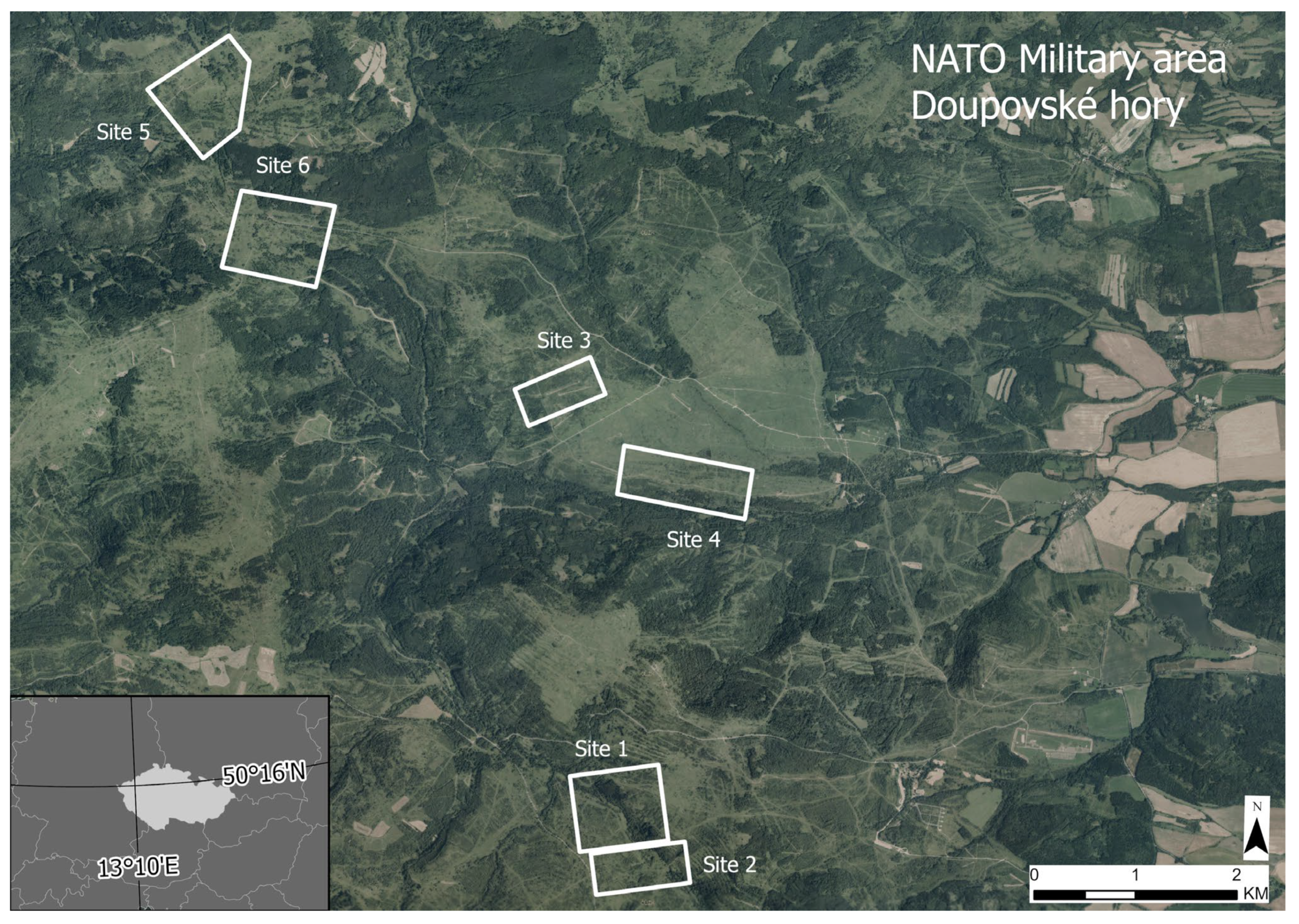
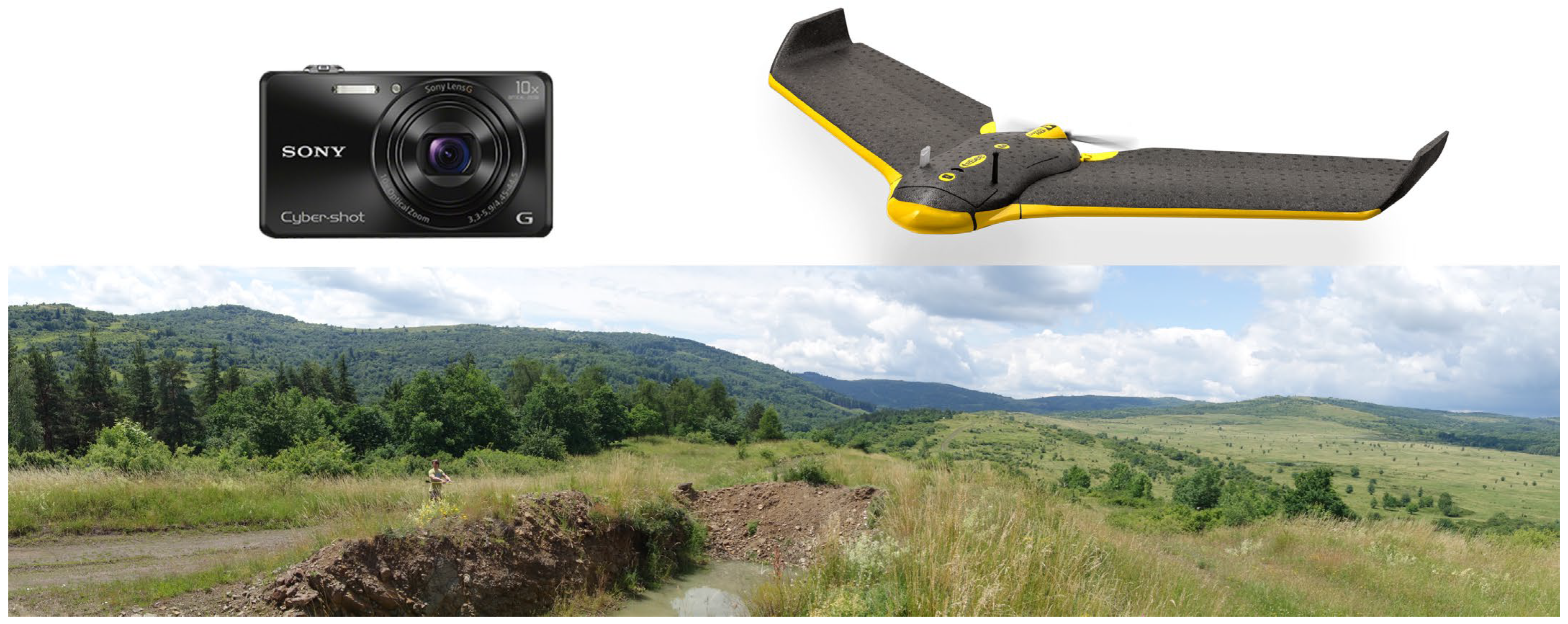
The study area, a NATO military training site, is situated in the western part of the Czech Republic (West Bohemia) in Doupovske hory; see Figure 1. The area is a landscape mosaic consisting of forests with casual forestry management (pine, larch, spruce, beech, oak, and ash) and large no-forest areas mainly covered by herbaceous vegetation and shrubs (hawthorn, alder, briar, blackthorn, and willow) that are mainly affected by military activities (Figure 2). The elevation of the predominantly hilly relief ranges between 364 and 933 m above mean sea level. The study area (approx. 630 km2) represents a nature-close area and is protected as an important Natura 2000 bird site. Six study sites with different environmental conditions, mainly situated in the shrubland with woody vegetation, were selected for this study (see Table 1).

Figure 1.
Study site overview.

Figure 2.
A broader view of the study area (bottom); the senseFly eBee equipped with a consumer-grade DSC-WX220 digital compact camera (top).

Table 1.
Detailed selected environmental parameters of individual study sites situated in the Doupovske hory military training area (derived from custom-ordered high density ALS data).
2.2. ALS, UAV, and Airborne Imagery Data Acquisition
The high-density (HD) airborne laser scanning (ALS) mission data were acquired on 10th September 2016 using an ALS70 scanner (Leica Geosystems, Aalen, Germany) mounted on an aircraft Cessna 402 (Cessna, Wichita, USA). The sensor wavelength was 1064 nm, and the scan field of view was 40°. The imagery was acquired from the altitude of 576–1141 m above ground with 70% side overlap. The acquired ALS point cloud covered an area of approximately 216 km2 and contained almost 486 million points, with a mean density of 20.61 pts/m2 (last return density of 15.54 pts/m2). Simultaneously with ALS data, RGB airborne imagery (AImg) with a 0.94 m pixel size was also acquired using Leica RCD30 medium format camera.
A low-density (LD) ALS dataset was acquired from the Czech Office for Surveying, Mapping, and Cadastre (ČÚZK). This dataset covers the whole territory of the Czech Republic; it was created during a nationwide campaign between 2009 and 2013 using an ALS mapping system called LiteMapper 6800 (IGI mbH, Kreuztal, Germany) with an RIEGL LMS-Q680 (RIEGL Laser Measurement Systems GmbH, Hoorn, Austria) scanner carried by an L-410 FG aircraft at an altitude of 1200–1400 m above ground. The study site was sensed in March 2011. Since 2016, the whole dataset has been available at a 2 m resolution raster (digital terrain and surface models separately). Only a DTM dataset called DMR 5G (Digital Terrain Model of the Czech Republic, 5th Generation) was used in this study.
UAV imagery was acquired on 27 June 2016 by a fixed-wing eBee Classic (senseFly, Cheseaux-sur-Lausanne, Switzerland) unmanned aerial vehicle (UAV) with a maximum take-off weight of approximately 0.8 kg and a wingspan of 0.96 m. The UAV was equipped with a consumer-grade DSC-WX220 digital compact camera (Sony, Tokyo, Japan), as detailed by Komárek et al. [37]. Flight lines were planned with the senseFly eMotion 2 ground station software (senseFly, Cheseaux-sur-Lausanne, Switzerland) with 70% side and 80% front overlaps. The average flight altitude was 120 m above ground level, and almost 1700 images were acquired during six flights at six different study locations (one flight per study location). Input datasets are summarized in Table 2.

Table 2.
Detailed characteristics of the four types of remote sensing-based input data used in the study.
The registration and georeferencing methodological framework for all input datasets was primarily based on ground control points (GCPs). Point clouds derived from airborne laser scanning (both HD and LD) were registered and georeferenced by data providers. In the case of the HD dataset, the declared mean horizontal error was lower than 0.15 m and the vertical error was lower than 0.11 m. Regarding the LD dataset, The mean horizontal error was 0.15 m and the vertical error was 0.18 m on bare ground and 0.3 m under vegetation.
2.3. Processing of Input Remote Sensing Data
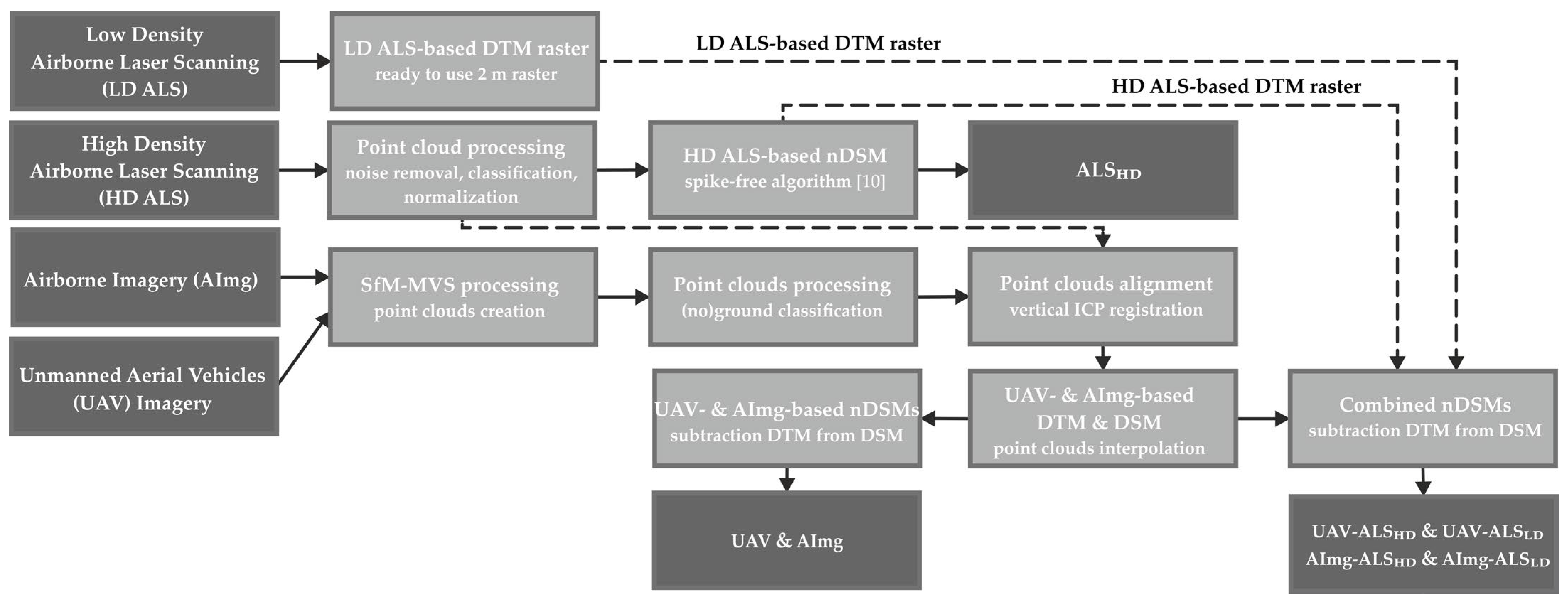
The methodological framework of input data processing was identical for all study sites. The LAStools software (rapidlasso GmbH, Gilching, Germany) was used for processing data acquired by HD ALS. The processing consisted of noise removal, point cloud classification (ground vs. woody vegetation), normalization, and raster interpolation using a specialized spike-free algorithm [21]. The spatial resolution of the nDSM was set to 0.25 m. The UAV-borne and airborne images were processed with the SfM-MVS methods utilizing five ground control points per site in Agisoft Metashape, version 1.7.3 (Agisoft LLC, Saint Petersburg, Russia). The GCPs were measured in the Czech national S-JTSK/Krovak East North (EPSG: 5514) and Baltic Sea vertical datum (EPSG: 5705) coordinate systems; no additional co-registration was needed. The mean horizontal error was lower than 0.20 m, and the vertical error was lower than 0.11 m.
2.4. Normalized Digital Surface Model (NDSM) Calculation
A normalized digital surface model represents the height of objects above the bare terrain. In the study sites, this mainly consisted of woody vegetation (trees, shrubs, etc.) and steppes with tall grass, with occasional military training area equipment. The identification of ground (DTM) and non-ground points (DSM) constituted a critical part of creating the nDSM. In the case of ALS, the DTM, DSM, and nDSM were directly created in the previous processing step in the LAStools software. For both UAV-borne and airborne imagery, Agisoft Metashape was used for the point cloud classification and for DTM, DSM, and orthomosaic interpolation (with spatial resolutions of 0.15 m for UAV and 0.94 m for AImg). No DSM was created from the LD ALS dataset because this dataset was 5 years older than the remaining datasets, which would have biased the results.
Finally, nDSMs were created by subtracting DTMs from DSMs in the ArcGIS software, version 10.7.1 (ESRI, Redlands, CA, USA). In addition to models created solely from UAV and airborne imagery, nDSMs combining their DSM with LD and HD ALS DTM were also created. In total, seven different nDSMs were used for further analysis. Detailed descriptions of the compared nDSMs are listed in Table 3. All outputs were computed in the Czech national S-JTSK/Krovak East North (EPSG: 5514) and Baltic Sea vertical datum (EPSG: 5705) coordinate systems.

Table 3.
Brief descriptions of seven calculated nDSMs and their remote sensing data inputs. Presented nDSMs were created based on the subtraction of the respective DTMs from DSMs.
2.5. Woody Plant Structure Analysis
The seven nDSMs (Table 3) were subsequently subjected to the automatic detection of woody plant tops using the individual tree detection (ITD) approach with local maxima filtering [38,39,40]. Based on the study location, 0–3 filtering steps with a kernel of 3 × 3 pixels and a local maxima searching window with a circular radius of 1.0, 1.5, or 2.0 m was applied [1]. In addition, the woody vegetation height was calculated (directly extracted from nDSMs) for each detected woody plant top in nDSMs. Both analyses were automated and performed using custom Python scripts in the ArcGIS software.
2.6. Statistical Analysis
The accuracy of nDSMs was assessed by comparing the number of detected woody plants (individual trees and shrubs) and their heights (m) with the reference. The study sites were overlaid with a 100 × 100 grid; subsequently, five squares within each area were randomly selected, and the reference number of individual trees/shrubs in each one was manually determined by the visual interpretation of the UAV-borne orthomosaics.
One hundred tree tops higher than 1 m (lower height was considered to be a possible noise), which were automatically detected in each model, were randomly selected at each study site. Using the mean absolute error (MAE) and percentage mean absolute error (%MAE) statistics, the heights of this woody vegetation were compared with a reference dataset created from proprietary ALSHD data owned by our university (high-density ALS datasets are generally considered to be the most accurate datasets for the determination of tree heights, e.g., Ganz et al. [16]). Both woody plant structure analyses were performed at two levels: (a) trees/shrubs and (b) trees (height over 5 m) vs. shrubs (below 5 m; this cut-off was established to match the criteria used in the CORINE Land Cover database). All statistical analyses were executed by custom scripts written in the R environment, version 3.5.1 (R Core Team, Vienna, Austria). The study workflow is schematically described in Figure 3.
Figure 3.
Description of the study workflow and the preparation of individual nDSMs.
3. Results
3.1. The Number of Detected Woody Plant Individuals
The comparison of the total numbers of automatically detected shrubs/trees to the manually determined reference (Table 4, upper row for each site) indicated that the total numbers of woody vegetation derived from models based on UAV imagery yielded better results than those based on airborne imagery. The models based on airborne imagery were less successful in detection (49.2%) than those based on UAV datasets (99.7%). However, combining AImg-based DSMs models with ALS-based DTMs led to a significant increase in detection success (AImg-ALSLD: 73.0%; AImg-ALSHD: 73.3%); for UAV-derived models, the detection remained close to 100% (UAV-ALSHD: 103.4%; UAV-ALSLD: 102.9%). The results also showed that the use of DTMs based on high- or low-density ALS for DSM height normalization did not lead to major differences in the success of tree detection.

Table 4.
The apparent success rate (%) of the automatic detection of the trees/shrubs over 1 m in height (upper rows) and the rate (%) of correctly automatically identified trees/shrubs (bottom rows) for individual sites and nDSMs.
At first sight, the results for many of the models utilizing photogrammetrically-derived methods shown in the Table 4 appeared to be very promising. However, a deeper analysis revealed that being satisfied with such seemingly high values could be premature, as the success rates close to 100% actually resulted from a combination of omission and commission errors of similar magnitudes. When looking only at the trees/shrubs that were located in the same positions by manual and automatic detection, the success rates dropped significantly (Table 4, the bottom row for each site). The actual numbers of woody plant tops correctly detected by the automated algorithm indicated that none of the tested nDSMs achieved an accuracy comparable with the ALSHD model (95.1%). The detection accuracies of all models for woody vegetation (i.e., trees and shrubs) slightly differed across study locations. The model based on UAV imagery yielded a better total detection accuracy (68.7%) than that based on the AImg nDSM (40.1%). When considering these adjusted success rates, we can see that the combinations of both DSMs with ALS DTMs yielded only negligible improvements for both the UAV and AImg models.
We can see that AImg-based models suffered from notable omission errors while in UAV-based models, commission and omission errors were of the approximately same magnitude (which led to the apparent high success rates; see Appendix A, Table A1 for a detailed breakdown of accuracy and errors in the detection of the numbers of treetops for individual sites).
3.2. Woody Vegetation Height Detection
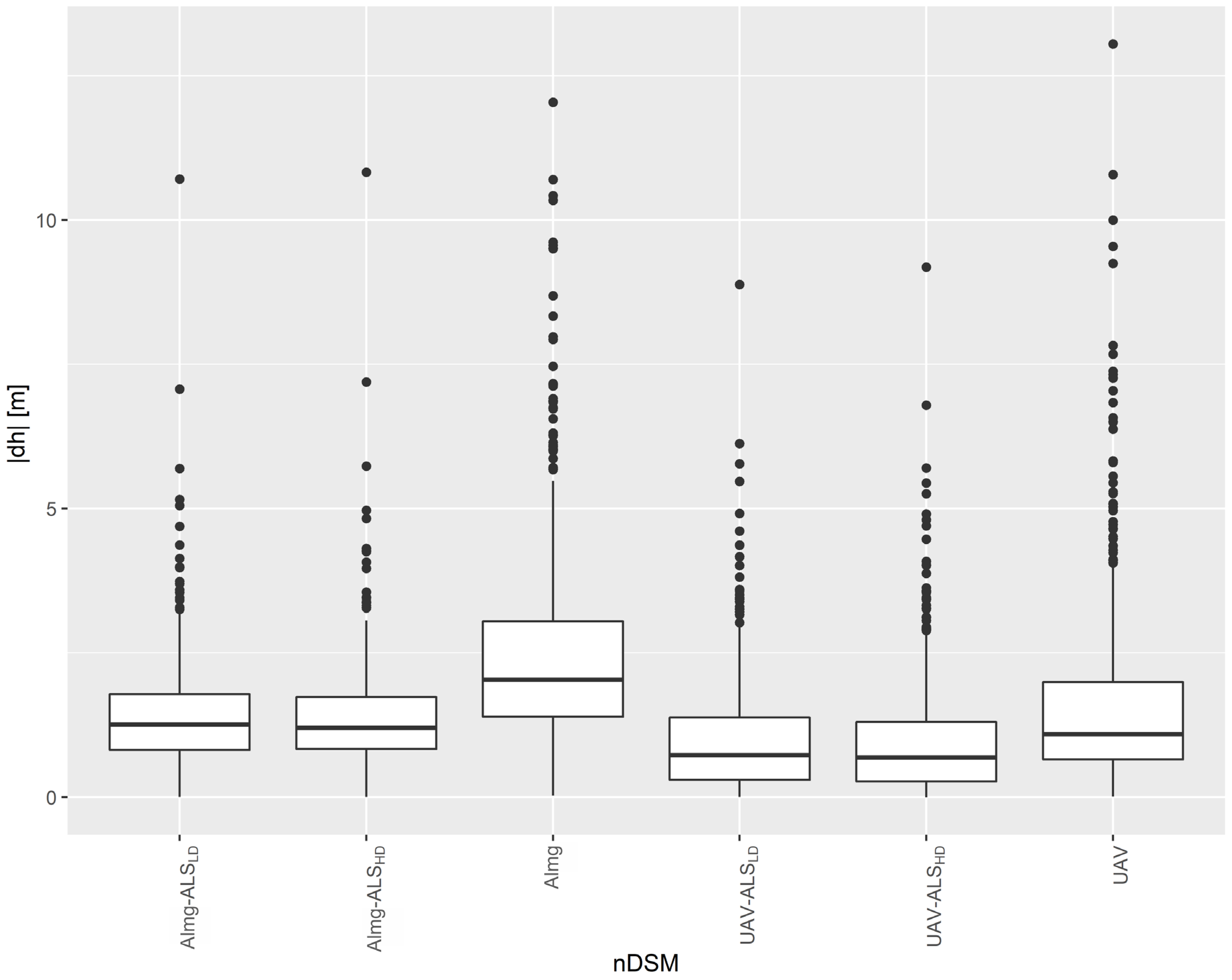
The results of woody vegetation height detection are presented in Table 5. The mean absolute errors (MAEs) of the UAV (MAE 1.6 m) and AImg (MAE 2.5 m) show the magnitude of the model’s difference from the ALSHD reference. However, combining these datasets with terrain data derived from ALS datasets led to an improvement of height accuracy. In this case, the most accurate UAV-based model (UAV-ALSHD) yielded an MAE of 1.0 m and the most accurate AImg-based model (AImg-ALSHD) yielded an MAE of 1.4 m. The differences between the use of ALSHD and ALSLD were minimal, which means that even outdated coarse ALS-based digital terrain models can be combined with UAV and AImg data to improve the quality of resulting nDSMs, even in study sites as heterogeneous as military training areas. Figure A3 (Appendix C) summarizes the basic descriptive statistics in height differences for individual models across all study sites (i.e., each box plot contains 600 randomly selected woody tops).

Table 5.
The height accuracy (mean absolute error—MAE, in meters; percentage mean absolute error—%MAE, in percentages) of woody plant tree tops detected from six nDSMs based on UAV and airborne imagery and their combinations with HD and LD ALS DTMs compared to the reference based on the HD ALS dataset.
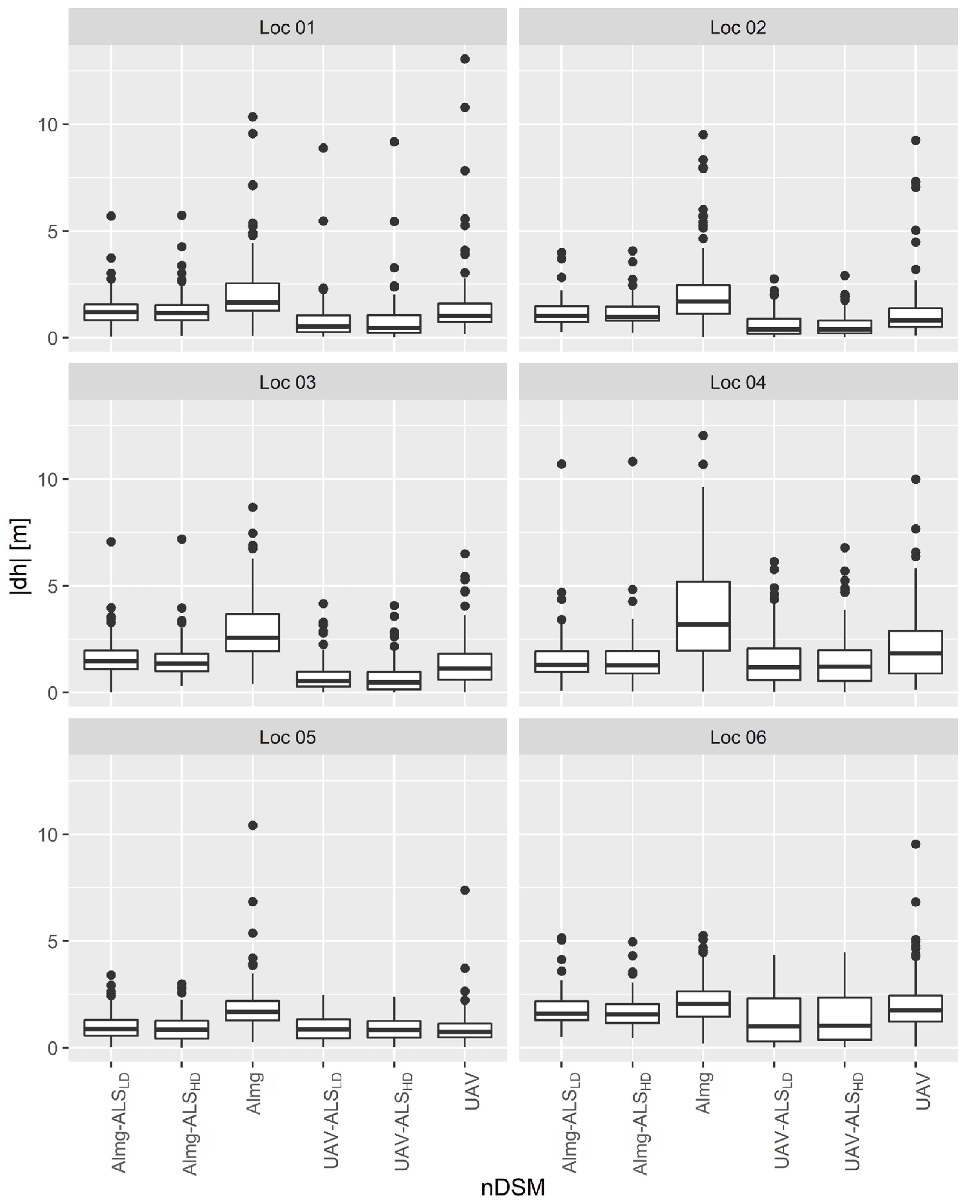
However, major differences in MAE between study sites were detected (Table 5). For UAV-based models, a significant dependence (R2 = 0.98) between the MAE and the mean height of woody vegetation on the particular sites (see Table 1) was detected. In other words, the %MAE remained more or less constant, contrary to AImg-based models (R2 = 0.23). Summaries of the descriptive statistics of both the absolute heights of woody vegetation and the differences from the reference dataset for individual sites and nDSMs are shown in Figure A1 and Figure A2. The results of the analyses of height accuracy and detection success according to the woody plant categories (tree/shrub) are shown in Table 6 and commented on in the Section 4.

Table 6.
The number of detected trees and shrubs (percentage of automatically correctly detected) and the height accuracy (percentage mean absolute error—%MAE) of trees, shrubs, and their combinations. Detected woody plants of 1–5 m were considered shrubs; those above 5 m were considered trees.
4. Discussion
4.1. The Number of Detected Woody Plant Individuals
At first sight, the overall detection accuracies appeared to be very good. However, our study demonstrates that reporting only those results would be problematic and that it is necessary to perform a deeper analysis when evaluating the true agreement between detection and reality (Table 4 and especially Table A1). After a closer look, the drop in accuracies of the UAV-based detection of individual trees/shrubs (apart from ALSHD) to 64.8–81.1 may appear to be unsatisfactory. On the other hand, it is necessary to point out that most studies on the automatic detection of shrubs/trees utilizing UAV/AImg (see below) have investigated the usability of such data and methods in economically exploited areas (forests, orchards, etc.)—not in highly heterogeneous, ecologically valuable, nature-close environments similar to the military area evaluated in this study, where it was even difficult to distinguish individual woody vegetation by visual interpretation. Figure 4 shows a graphic example of the detection success for individual models at Site 5. Other studies utilizing UAV-based nDSMs have also reported variances in observed successes. Mohan et al. [41] detected individual trees with an accuracy of 80% using UAV-borne data combined with variable filtering and the moving window technique. A similar accuracy was reported by Liu et al. [42], who achieved an 85% success in the detection of trees in urban areas using ALS data. In contrast, Surový et al. [32] reported 43–80% success rates and Nevalainen et al. [43] reported 40–95% success rates depending on the characteristics of the study sites (in particular, on the plant species constituting the vegetation cover).
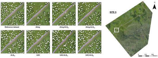
Figure 4.
Examples of the individual woody plant detections for seven created nDSMs and the reference orthomosaic created by visual interpretation (top left corner) on the sample of Site 5. White dots represent individual detected shrubs and trees. White frame represents a subset of the study Site 5.
Table A1 describes detailed values of ITD accuracies. Besides the overall accuracy, the numbers of omitted and committed shrub- and tree-tops are also important. The omission of ITD is also associated with the height accuracy. As the height of low woody vegetation (mainly shrubs) is very similar to that of noise generated during nDSM calculations (subtraction of DTM from DSM), they are often incorrectly eliminated during ITD processing. The number of omitted tops decreases with the improving height accuracy of nDSMs; however, the improving accuracy also results in an increased number of commissions (mainly in shrubland with sparse woody vegetation). The detection success probably depends on both the input data and the chosen algorithm. In this study, we aimed to evaluate the possibilities offered by various RS input data. For this reason, we did not attempt to search for the best possible ITD algorithm but rather used the most widely used one with a fixed local maxima search window. Therefore, there are ways that could likely lead to ITD result improvements through (a) the use of adaptive local maxima search window or (b) the involvement of spectral information.
4.2. Woody Vegetation Height Detection
The height differences between the UAV-borne/airborne data and the ALSHD reference dataset represented by the MAE were small enough to be of value for practical applications related to the woody vegetation structures, in particular when ALS data are used for terrain characterization (Table 5 and Figure A2 in the Appendix B). The overall absolute MAEs of 1.0 m were the same for both most accurate nDSMs, which is very promising and comparable with the accuracy of in situ field measurements; for example, [16] reported an RMSE of 1.0 m when using a Vertex clinometer. Their study, however, focused on typical European forests, not on woody vegetation as heterogeneous as in our study area. In their study, an RMSE of 1.1 m (mean error: −1.0 m) was reported for a UAV-based nDSM and an RMSE of 2.9 m (mean error: −2.7) was reported for an AImg-based model. The total height MAEs for the UAV-based nDSM and the AImg model in our study were 1.6 and 2.5 m, respectively.
Our research yielded satisfactory results, which are similar to those of other studies focusing on the validation of the height accuracy of UAV-based nDSMs against field measurements. For example, Tuominen et al. [44] reported a tree stand height %RMSE of approx. 10%, which differed among tree species. On the other hand, Puliti et al. [45] achieved a %RMSE of approx. 13.3%; the RMSE difference was around 1.4 m. Wallace et al. [46] measured the tree height with an RMSE of 1.30 m for SfM input data in a eucalypt forest in Tasmania. Panagiotidis et al. [1] reported MAEs of 2.62 and 2.88 m (RMSEs of 3.00 and 3.08 m; %RMSEs of 11.42 and 12.62%) in the forests of the Czech Republic. Zarco-Tejada et al. [47] reported an RMSE of 0.35 m (%RMSE: 11.50%) and Díaz-Varela et al. [48] reported RMSEs ranging from 0.20 to 0.45 m (%RMSE: 6.55–19.24%) in (mainly) olive orchards in Spain. Surový et al. [32] reported RMSEs of 0.6–1.1 m in Portuguese plantations with cork oak, holm oak, and umbrella pine.
Unlike the work of Surový et al. [32], the MAEs in our study were higher at certain sites (in particular, Sites 4 and 6) while the %MAE remained more or less unchanged. In other words, although the relative accuracy remained the same across sites, the absolute differences increased with tree/shrub height. It should be also noted that the variability in the height of woody plant tops in Sites 4 and 6 was generally higher than in the remaining sites (see Figure A1 in the Appendix B). This was not observed in the case of airborne imagery. We assume that this was due to the coarser spatial resolution of airborne imagery compared to that of UAVs (0.94 vs. 0.15 m, respectively). A coarser resolution can often completely fail to identify shrubby vegetation due to its low height and relatively small diameter or, if recognized, may not support the precise identification of the tree/shrub top and calculate a mean height of the area instead.
4.3. Tree vs. Shrub Height Accuracy and Detection Success
A comparison of the detection success between trees (height over 5 m) and shrubs (below 5 m) is an interesting and unique analysis that had not been performed previously. When considering the accuracies of trees and shrubs separately, we could see that throughout the models, the relative accuracy was better for trees than for shrubs (Table 6). The relatively poorer detection of shrubs in the purely UAV- or AV-based models was likely caused by the fact that it is highly difficult to distinguish a low shrub from the surrounding terrain/herbaceous vegetation in such a model; additionally, the canopy in shrub thickets tends to smoothen out minor terrain undulations, which made the individual shrub tops more distinct after the correction for the ALS-based DTM. The tree height was detected with better relative accuracy than shrub height in all cases (%MAE). Still, none of the methods of individual tree detection yielded accuracies similar to ALSHD. For this reason, we propose that for such heterogeneous, nature-close areas with dense tree stands and thickets, it might be more reasonable to detect the total woody plant area rather than the number of shrub/tree individuals.
4.4. UAV-Based DSM and ALS-Based DTM Fusion
Combining UAV-borne or airborne DSMs with ALS-based DTM represents a successful solution for the problems of heterogeneous environments such as our study area. The fact that there were no major differences between the use of the terrain model derived from the expensive custom-ordered “high density” ALS (ALSHD) and of the DTM derived from the nationwide freely available low-density ALS (ALSLD) is an important result of our study; even more important is that the point cloud densities (20.61 vs. 2.00 pts/m2) and acquisition dates (2016 vs. 2011) were different, with the ALSLD being more outdated. In our study, ALSLD was sensed in the leaf-off period (March), which is typical of nationwide ALS campaigns predominantly aimed at obtaining topographic information, while ALSHD was acquired in the vegetation period (September), which was necessary for the acquisition of suitable data for accurate vegetation models. In any case, our results indicated that even in sites as heterogeneous as our study area with frequent disturbances, digital surface models built from up-to-date UAV/airborne data can be successfully combined with older ALS-based DTMs, even those with low density. The time of data acquisition is also important for accurate DSM construction [49], with the vegetation period preferred for this purpose. Therefore, the imagery was sensed in June (UAV) and September (ALSHD and AImg, respectively).
4.5. Landscape/Vegetation Patterns Classification
Standard approaches for the classification of landscape patterns (in terms of vegetation) use both spectral and vertical RS-based information. The most common landscape pattern analyses typically use image interpretation/classification or field measurement methods [20]. Bakx et al. [23] predominantly focused on the use of ALS for deriving the characteristics of vegetation structures. ALS-based vegetation properties thus demonstrably represent information beneficial for analyses of landscape patterns; however, based on our results, we can propose that UAV-based characteristics of woody vegetation structures could be a valuable addition for such analyses. The promising accuracy of calculated UAV-based woody plant structure properties (see Table 6), particularly in combination with (even outdated and low-resolution) ALS data, is indicative of their possible benefit for further landscape spatial pattern analyses.
For illustration and a brief evaluation of the possible benefit of the combination of UAV imagery and freely available nationwide ALS data, we calculated the percentage of the woody plant area, which constitutes a common characteristic of vegetation structures. From the results presented in Table 7, it is evident that the values of both parameters were close enough to values obtained from a model solely derived from expensive high-density ALS data.

Table 7.
The application of UAV-ALSLD nDSM for the estimation of vegetation structure characteristics compared to ALSHD as reference. The area of woody vegetation represents a percentage of vegetation cover (trees and shrubs). Woody plants of 1–5 m were classified as shrubs, and those above 5 m were classified as trees. Vegetation property calculations are presented in Table 5 and Table 6.
5. Conclusions
Our study was aimed to evaluate the potential of UAV- and AImg-based nDSMs for the estimation of tree/shrub heights and the detection of individual woody vegetation. We confirmed the usability of UAV-borne and airborne imagery outside economically exploited areas (forests, orchards, etc.). Our results prove that UAV-borne imagery can provide valuable vegetation structure data for analyses of local, dynamically changing, highly heterogeneous, nature-close environments; thus, it can offer an alternative to expensive high-tech solutions such as ALS on a suitable spatial scale. In addition, we combined DSMs based on UAV-borne and airborne imagery with ALS-based DTMs. Their fusion significantly increased the accuracy of (especially) woody plant height estimation (trees and shrubs). It is also possible that the use of spectral information from UAVs could further improve the success of woody plant detection, which is a potentially promising direction for further research. The results also confirmed that even coarse and outdated ALS datasets (ALSLD in the study) can be a valuable source of DTMs for UAV- or AImg-based nDSMs, capable of improving height data detection to a degree comparable with laborious manual measurement. Additionally, up-to-date UAV- and AImg-based DSMs can be also beneficial for updating outdated ALS-based DSMs.
Author Contributions
All authors contributed in a substantial way to the manuscript. T.K. and J.K. conceived, designed, and performed the experiment and wrote significant parts of the manuscript. T.K. was responsible for project leadership and management. J.K. and P.K. contributed to the acquisition of UAV imagery. P.K. and J.K. processed all input remote sensing data. J.M. performed the formal analysis and statistical evaluation. T.K. and J.K. were responsible for project funding. All authors have read and agreed to the published version of the manuscript.
Funding
This research was supported by the Technology Agency of the Czech Republic under the grant Nos. CK02000203, TJ02000283, SS02030018, and TP01010050.
Data Availability Statement
The data that support the findings of this study are openly available in the “figshare” repository at doi.org10.6084/m9.figshare.16559109 (accessed on 12 March 2022).
Acknowledgments
We would like to thank Ondřej Lagner and Jiří Prošek for help with UAV imagery acquisition, Michal Fogl for help with ALS data processing, and Petra Šímová for her help with ALS data procurement and valuable comments. Many thanks also to Jarek Janošek for helpful comments. The research was supported by the Action CA17134 SENSECO (Optical synergies for spatiotemporal sensing of scalable ecophysiological traits) funded by COST (European Cooperation in Science and Technology, www.cost.eu, accessed on 12 March 2022).
Conflicts of Interest
The authors declare no conflict of interest.
Appendix A

Table A1.
Summary of individual tree detection (ITD) results of woody vegetation in six study locations.
Table A1.
Summary of individual tree detection (ITD) results of woody vegetation in six study locations.
| ALSHD | AImg | AImg-ALSLD | AImg-ALSHD | UAV | UAV-ALSLD | UAV-ALSHD | ||
|---|---|---|---|---|---|---|---|---|
| Site 01 | Detected | 1183 | 596 | 799 | 802 | 1164 | 1018 | 1138 |
| Reference | 1214 | 1214 | 1214 | 1214 | 1214 | 1214 | 1214 | |
| True | 1128 | 499 | 612 | 610 | 840 | 790 | 833 | |
| Omission | 86 | 715 | 602 | 604 | 374 | 424 | 381 | |
| Commission | 55 | 97 | 187 | 192 | 324 | 228 | 305 | |
| Accuracy (%) | 92.9 | 41.1 | 50.4 | 50.3 | 69.2 | 65.1 | 68.6 | |
| Site 02 | Detected | 976 | 508 | 653 | 636 | 815 | 849 | 828 |
| Reference | 946 | 946 | 946 | 946 | 946 | 946 | 946 | |
| True | 898 | 444 | 468 | 447 | 617 | 656 | 661 | |
| Omission | 48 | 502 | 478 | 499 | 329 | 290 | 285 | |
| Commission | 78 | 64 | 185 | 189 | 198 | 193 | 167 | |
| Accuracy (%) | 94.9 | 46.9 | 49.5 | 47.2 | 65.2 | 69.3 | 69.9 | |
| Site 03 | Detected | 1256 | 369 | 949 | 886 | 1096 | 1001 | 1224 |
| Reference | 1215 | 1215 | 1215 | 1215 | 1215 | 1215 | 1215 | |
| True | 1200 | 301 | 653 | 628 | 787 | 780 | 914 | |
| Omission | 15 | 914 | 562 | 587 | 428 | 435 | 301 | |
| Commission | 56 | 68 | 296 | 258 | 309 | 221 | 310 | |
| Accuracy (%) | 98.8 | 24.8 | 53.7 | 51.7 | 64.8 | 64.2 | 75.2 | |
| Site 04 | Detected | 1016 | 603 | 799 | 851 | 1133 | 1582 | 1304 |
| Reference | 1023 | 1023 | 1023 | 1023 | 1023 | 1023 | 1023 | |
| True | 972 | 430 | 551 | 552 | 688 | 705 | 669 | |
| Omission | 51 | 593 | 472 | 471 | 335 | 318 | 354 | |
| Commission | 44 | 173 | 248 | 299 | 445 | 877 | 635 | |
| Accuracy (%) | 95.0 | 42.0 | 53.9 | 54.0 | 67.3 | 68.9 | 65.4 | |
| Site 05 | Detected | 842 | 464 | 775 | 633 | 975 | 851 | 791 |
| Reference | 825 | 825 | 825 | 825 | 825 | 825 | 825 | |
| True | 794 | 370 | 472 | 460 | 669 | 636 | 629 | |
| Omission | 31 | 455 | 353 | 365 | 156 | 189 | 196 | |
| Commission | 48 | 94 | 303 | 173 | 306 | 215 | 162 | |
| Accuracy (%) | 96.2 | 44.8 | 57.2 | 55.76 | 81.1 | 77.1 | 76.2 | |
| Site 06 | Detected | 853 | 436 | 442 | 631 | 852 | 959 | 943 |
| Reference | 831 | 831 | 831 | 831 | 831 | 831 | 831 | |
| True | 767 | 383 | 368 | 415 | 555 | 588 | 584 | |
| Omission | 64 | 448 | 463 | 416 | 276 | 243 | 247 | |
| Commission | 86 | 53 | 74 | 216 | 297 | 371 | 359 | |
| Accuracy (%) | 92.3 | 46.1 | 44.2 | 49.9 | 66.8 | 70.8 | 70.3 | |
| Overall | Detected | 6126 | 2976 | 4237 | 4439 | 6035 | 6260 | 6228 |
| Reference | 6054 | 6054 | 6054 | 6054 | 6054 | 6054 | 6054 | |
| True | 5759 | 2427 | 3124 | 3112 | 4156 | 4155 | 4209 | |
| Omission | 295 | 3627 | 2988 | 2942 | 1898 | 1899 | 1764 | |
| Commission | 367 | 549 | 1171 | 1327 | 1879 | 2105 | 1938 | |
| Accuracy (%) | 95.1 | 40.1 | 51.6 | 51.4 | 68.7 | 68.6 | 70.9 |
Appendix B
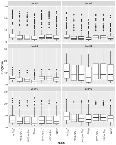
Figure A1.
Box-plots displaying quartile characteristics (median, Q25, and Q75) of the absolute nDSM heights for each study location. For each location, 100 randomly selected woody plant tops were used. Black dots represent outliers.
Figure A1.
Box-plots displaying quartile characteristics (median, Q25, and Q75) of the absolute nDSM heights for each study location. For each location, 100 randomly selected woody plant tops were used. Black dots represent outliers.
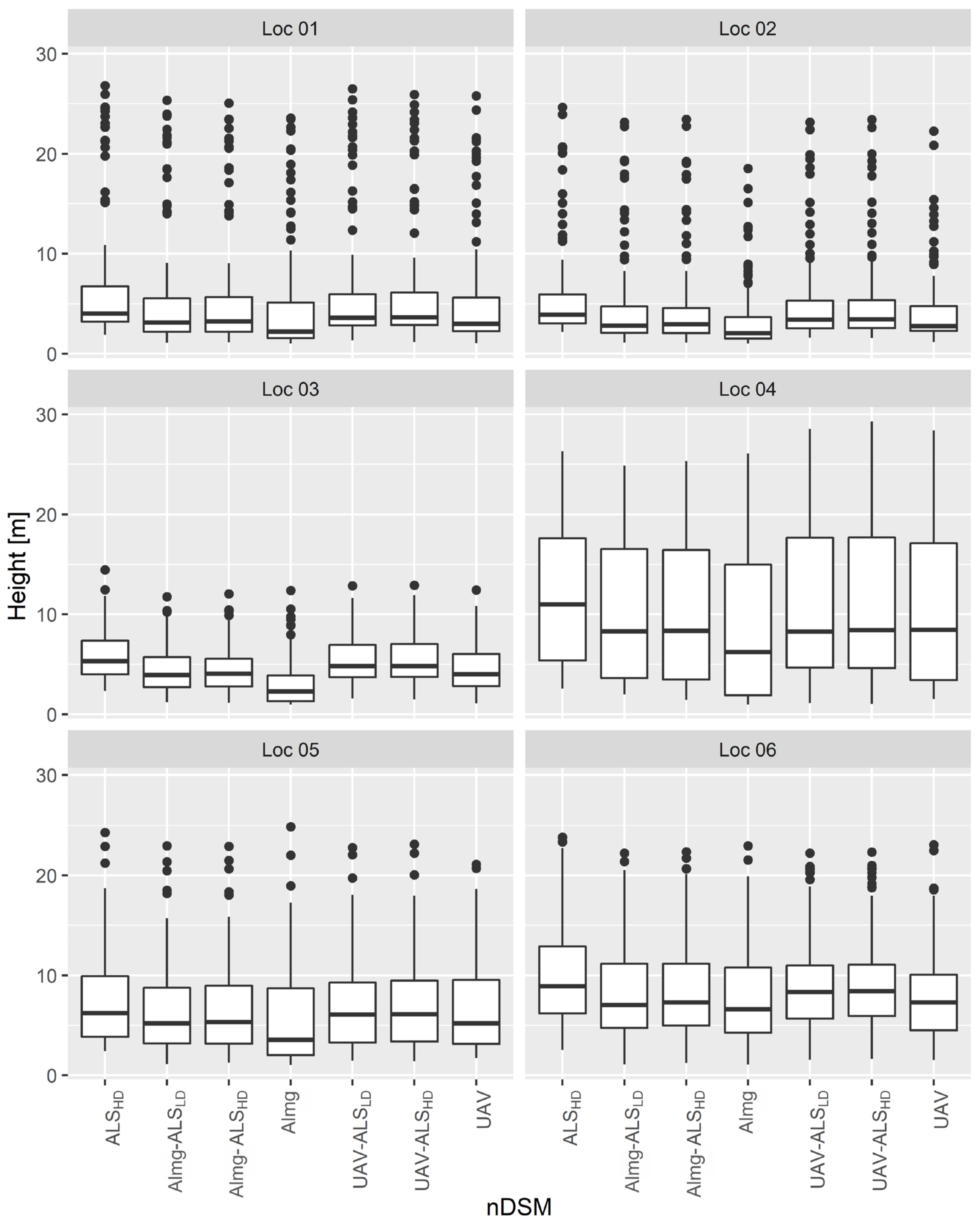
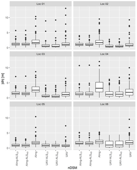
Figure A2.
Box-plots displaying quartile characteristics (median, Q25, and Q75) of nDSM height differences for individual study locations. For each location, 100 randomly selected woody plant tops were used. Black dots represent outliers.
Figure A2.
Box-plots displaying quartile characteristics (median, Q25, and Q75) of nDSM height differences for individual study locations. For each location, 100 randomly selected woody plant tops were used. Black dots represent outliers.
Appendix C
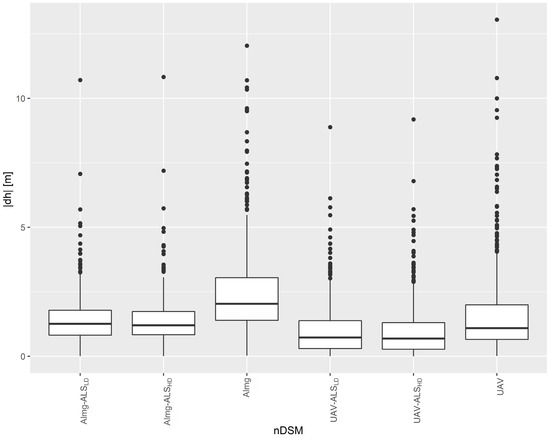
Figure A3.
Box-plots of summary quartile characteristics (median, Q25, and Q75) of nDSM height differences from ALSHD reference for all study locations. For every nDSM, 600 randomly selected woody plant tops were used. Black dots represent outliers.
Figure A3.
Box-plots of summary quartile characteristics (median, Q25, and Q75) of nDSM height differences from ALSHD reference for all study locations. For every nDSM, 600 randomly selected woody plant tops were used. Black dots represent outliers.
References
- Panagiotidis, D.; Abdollahnejad, A.; Surový, P.; Chiteculo, V. Determining Tree Height and Crown Diameter from High-Resolution UAV Imagery. Int. J. Remote Sens. 2017, 38, 2392–2410. [Google Scholar] [CrossRef]
- Lelli, C.; Bruun, H.H.; Chiarucci, A.; Donati, D.; Frascaroli, F.; Fritz, Ö.; Goldberg, I.; Nascimbene, J.; Tøttrup, A.P.; Rahbek, C.; et al. Biodiversity Response to Forest Structure and Management: Comparing Species Richness, Conservation Relevant Species and Functional Diversity as Metrics in Forest Conservation. For. Ecol. Manag. 2019, 432, 707–717. [Google Scholar] [CrossRef]
- Bohn, F.J.; Huth, A. The Importance of Forest Structure to Biodiversity-Productivity Relationships. R. Soc. Open Sci. 2017, 4, 160521. [Google Scholar] [CrossRef] [PubMed] [Green Version]
- Matsumoto, H.; Ohtani, M.; Washitani, I. Tree Crown Size Estimated Using Image Processing: A Biodiversity Index for Sloping Subtropical Broad-Leaved Forests. Trop. Conserv. Sci. 2017, 10, 1940082917721787. [Google Scholar] [CrossRef] [Green Version]
- Scherrer, D.; Massy, S.; Meier, S.; Vittoz, P.; Guisan, A. Assessing and Predicting Shifts in Mountain Forest Composition across 25 Years of Climate Change. Divers. Distrib. 2017, 23, 517–528. [Google Scholar] [CrossRef] [Green Version]
- Fujimoto, A.; Haga, C.; Matsui, T.; Machimura, T.; Hayashi, K.; Sugita, S.; Takagi, H. An End to End Process Development for UAV-SfM Based Forest Monitoring: Individual Tree Detection, Species Classification and Carbon Dynamics Simulation. Forests 2019, 10, 680. [Google Scholar] [CrossRef] [Green Version]
- Klouček, T.; Komárek, J.; Surový, P.; Hrach, K.; Janata, P.; Vašíček, B. The Use of UAV Mounted Sensors for Precise Detection of Bark Beetle Infestation. Remote Sens. 2019, 11, 1561. [Google Scholar] [CrossRef] [Green Version]
- Kašpar, V.; Hederová, L.; Macek, M.; Müllerová, J.; Prošek, J.; Surový, P.; Wild, J.; Kopecký, M. Temperature Buffering in Temperate Forests: Comparing Microclimate Models Based on Ground Measurements with Active and Passive Remote Sensing. Remote Sens. Environ. 2021, 263, 112522. [Google Scholar] [CrossRef]
- Getzin, S.; Nuske, R.S.; Wiegand, K. Using Unmanned Aerial Vehicles (UAV) to Quantify Spatial Gap Patterns in Forests. Remote Sens. 2014, 6, 6988–7004. [Google Scholar] [CrossRef] [Green Version]
- Lin, J.; Wang, M.; Ma, M.; Lin, Y. Aboveground Tree Biomass Estimation of Sparse Subalpine Coniferous Forest with UAV Oblique Photography. Remote Sens. 2018, 10, 1849. [Google Scholar] [CrossRef] [Green Version]
- Reif, J.; Marhoul, P.; Čížek, O.; Konvička, M. Abandoned Military Training Sites Are an Overlooked Refuge for At-Risk Open Habitat Bird Species. Biodivers. Conserv. 2011, 20, 3645–3662. [Google Scholar] [CrossRef]
- Carvajal-Ramírez, F.; da Silva, J.R.M.; Agüera-Vega, F.; Martínez-Carricondo, P.; Serrano, J.; Moral, F.J. Evaluation of Fire Severity Indices Based on Pre- and Post-Fire Multispectral Imagery Sensed from UAV. Remote Sens. 2019, 11, 993. [Google Scholar] [CrossRef] [Green Version]
- Bušek, O.; Reif, J. The Potential of Military Training Areas for Bird Conservation in a Central European Landscape. Acta Oecologica 2017, 84, 34–40. [Google Scholar] [CrossRef]
- Svenningsen, S.R.; Levin, G.; Perner, M.L. Military Land Use and the Impact on Landscape: A Study of Land Use History on Danish Defence Sites. Land Use Policy 2019, 84, 114–126. [Google Scholar] [CrossRef]
- Hamraz, H.; Contreras, M.A.; Zhang, J. Vertical Stratification of Forest Canopy for Segmentation of Understory Trees within Small-Footprint Airborne LiDAR Point Clouds. ISPRS J. Photogramm. Remote Sens. 2017, 130, 385–392. [Google Scholar] [CrossRef] [Green Version]
- Ganz, S.; Käber, Y.; Adler, P. Measuring Tree Height with Remote Sensing-a Comparison of Photogrammetric and LiDAR Data with Different Field Measurements. Forests 2019, 10, 694. [Google Scholar] [CrossRef] [Green Version]
- Komárek, J. The Perspective of Unmanned Aerial Systems in Forest Management: Do We Really Need Such Details? Appl. Veg. Sci. 2020, 23, 718–721. [Google Scholar] [CrossRef]
- White, J.C.; Wulder, M.A.; Vastaranta, M.; Coops, N.C.; Pitt, D.; Woods, M. The Utility of Image-Based Point Clouds for Forest Inventory: A Comparison with Airborne Laser Scanning. Forests 2013, 4, 518–536. [Google Scholar] [CrossRef] [Green Version]
- Puliti, S.; Dash, J.P.; Watt, M.S.; Breidenbach, J.; Pearse, G.D. A Comparison of UAV Laser Scanning, Photogrammetry and Airborne Laser Scanning for Precision Inventory of Small-Forest Properties. Forestry 2020, 93, 150–162. [Google Scholar] [CrossRef]
- Bergen, K.M.; Goetz, S.J.; Dubayah, R.O.; Henebry, G.M.; Hunsaker, C.T.; Imhoff, M.L.; Nelson, R.F.; Parker, G.G.; Radeloff, V.C. Remote Sensing of Vegetation 3-D Structure for Biodiversity and Habitat: Review and Implications for Lidar and Radar Spaceborne Missions. J. Geophys. Res. Biogeosci. 2009, 114, G00E06. [Google Scholar] [CrossRef] [Green Version]
- Khosravipour, A.; Skidmore, A.K.; Isenburg, M. Generating Spike-Free Digital Surface Models Using LiDAR Raw Point Clouds: A New Approach for Forestry Applications. Int. J. Appl. Earth Obs. Geoinf. 2016, 52, 104–114. [Google Scholar] [CrossRef]
- Khosravipour, A.; Skidmore, A.K.; Isenburg, M.; Wang, T.; Hussin, Y.A. Generating Pit-Free Canopy Height Models from Airborne Lidar. Photogramm. Eng. Remote Sens. 2014, 80, 863–872. [Google Scholar] [CrossRef]
- Bakx, T.R.M.; Koma, Z.; Seijmonsbergen, A.C.; Kissling, W.D. Use and Categorization of Light Detection and Ranging Vegetation Metrics in Avian Diversity and Species Distribution Research. Divers. Distrib. 2019, 25, 1045–1059. [Google Scholar] [CrossRef] [Green Version]
- Moudrý, V.; Klápště, P.; Fogl, M.; Gdulová, K.; Barták, V.; Urban, R. Assessment of LiDAR Ground Filtering Algorithms for Determining Ground Surface of Non-Natural Terrain Overgrown with Forest and Steppe Vegetation. Measurement 2020, 150, 107047. [Google Scholar] [CrossRef]
- Salach, A.; Bakula, K.; Pilarska, M.; Ostrowski, W.; Górski, K.; Kurczynski, Z. Accuracy Assessment of Point Clouds from LidaR and Dense Image Matching Acquired Using the UAV Platform for DTM Creation. ISPRS Int. J. Geo-Inf. 2018, 7, 342. [Google Scholar] [CrossRef] [Green Version]
- Wallace, L.; Bellman, C.; Hally, B.; Hernandez, J.; Jones, S.; Hillman, S. Assessing the Ability of Image Based Point Clouds Captured from a UAV to Measure the Terrain in the Presence of Canopy Cover. Forests 2019, 10, 284. [Google Scholar] [CrossRef] [Green Version]
- Klápště, P.; Fogl, M.; Barták, V.; Gdulová, K.; Urban, R.; Moudrý, V. Sensitivity Analysis of Parameters and Contrasting Performance of Ground Filtering Algorithms with UAV Photogrammetry-Based and LiDAR Point Clouds. Int. J. Digit. Earth 2020, 13, 1672–1694. [Google Scholar] [CrossRef]
- Klouček, T.; Lagner, O.; Šímová, P. How Does Data Accuracy Influence the Reliability of Digital Viewshed Models? A Case Study with Wind Turbines. Appl. Geogr. 2015, 64, 46–54. [Google Scholar] [CrossRef]
- Lagner, O.; Klouček, T.; Šímová, P. Impact of Input Data (in) Accuracy on Overestimation of Visible Area in Digital Viewshed Models. PeerJ 2018, 6, e4835. [Google Scholar] [CrossRef]
- Ke, Y.; Quackenbush, L.J. A Review of Methods for Automatic Individual Tree-Crown Detection and Delineation from Passive Remote Sensing. Int. J. Remote Sens. 2011, 32, 4725–4747. [Google Scholar] [CrossRef]
- Vauhkonen, J.; Ene, L.; Gupta, S.; Heinzel, J.; Holmgren, J.; Pitkänen, J.; Solberg, S.; Wang, Y.; Weinacker, H.; Hauglin, K.M.; et al. Comparative Testing of Single-Tree Detection Algorithms under Different Types of Forest. Forestry 2012, 85, 27–40. [Google Scholar] [CrossRef] [Green Version]
- Surový, P.; Almeida Ribeiro, N.; Panagiotidis, D. Estimation of Positions and Heights from UAV-Sensed Imagery in Tree Plantations in Agrosilvopastoral Systems. Int. J. Remote Sens. 2018, 39, 4786–4800. [Google Scholar] [CrossRef]
- Kuželka, K.; Slavík, M.; Surový, P. Very High Density Point Clouds from UAV Laser Scanning for Automatic Tree Stem Detection and Direct Diameter Measurement. Remote Sens. 2020, 12, 1236. [Google Scholar] [CrossRef] [Green Version]
- Antonello, A.; Franceschi, S.; Floreancig, V.; Comiti, F.; Tonon, G. Application of a Pattern Recognition Algorithm for Single Tree Detection from LiDAR Data. Int. Arch. Photogramm. Remote Sens. Spat. Inf. Sci. 2017, 42, 27–33. [Google Scholar] [CrossRef] [Green Version]
- Salamí, E.; Barrado, C.; Pastor, E. UAV Flight Experiments Applied to the Remote Sensing of Vegetated Areas. Remote Sens. 2014, 6, 11051–11081. [Google Scholar] [CrossRef] [Green Version]
- Torresan, C.; Berton, A.; Carotenuto, F.; Di Gennaro, S.F.; Gioli, B.; Matese, A.; Miglietta, F.; Vagnoli, C.; Zaldei, A.; Wallace, L. Forestry Applications of UAVs in Europe: A Review. Int. J. Remote Sens. 2017, 38, 2427–2447. [Google Scholar] [CrossRef]
- Komárek, J.; Klouček, T.; Prošek, J. The Potential of Unmanned Aerial Systems: A Tool towards Precision Classification of Hard-to-Distinguish Vegetation Types? Int. J. Appl. Earth Obs. Geoinf. 2018, 71, 9–19. [Google Scholar] [CrossRef]
- Chen, Q.; Baldocchi, D.; Gong, P.; Kelly, M. Isolating Individual Trees in a Savanna Woodland Using Small Footprint LIDAR Data Isolating Individual Trees in a Savanna Woodland Using Small Footprint Lidar Data. Photogramm. Eng. Remote Sens. 2006, 72, 923–932. [Google Scholar] [CrossRef] [Green Version]
- Koch, B.; Heyder, U.; Weinacker, H. Detection of Individual Tree Crowns in Airborne Lidar Data. Photogramm. Eng. Remote Sens. 2006, 72, 357–363. [Google Scholar] [CrossRef] [Green Version]
- Popescu, S.C.; Wynne, R.H.; Nelson, R.F. Estimating Plot-Level Tree Heights with Lidar: Local Filtering with a Canopy-Height Based Variable Window Size. Comput. Electron. Agric. 2002, 37, 71–95. [Google Scholar] [CrossRef]
- Mohan, M.; Silva, C.A.; Klauberg, C.; Jat, P.; Catts, G.; Cardil, A.; Hudak, A.T.; Dia, M. Individual Tree Detection from Unmanned Aerial Vehicle (UAV) Derived Canopy Height Model in an Open Canopy Mixed Conifer Forest. Forests 2017, 8, 340. [Google Scholar] [CrossRef] [Green Version]
- Liu, J.; Shen, J.; Zhao, R.; Xu, S. Extraction of Individual Tree Crowns from Airborne LiDAR Data in Human Settlements. Math. Comput. Model. 2013, 58, 524–535. [Google Scholar] [CrossRef]
- Nevalainen, O.; Honkavaara, E.; Tuominen, S.; Viljanen, N.; Hakala, T.; Yu, X.; Hyyppä, J.; Saari, H.; Pölönen, I.; Imai, N.N.; et al. Individual Tree Detection and Classification with UAV-Based Photogrammetric Point Clouds and Hyperspectral Imaging. Remote Sens. 2017, 9, 185. [Google Scholar] [CrossRef] [Green Version]
- Tuominen, S.; Balazs, A.; Honkavaara, E.; Pölönen, I.; Saari, H.; Hakala, T.; Viljanen, N. Hyperspectral UAV-Imagery and Photogrammetric Canopy Height Model in Estimating Forest Stand Variables. Silva Fenn. 2017, 51, 7721. [Google Scholar] [CrossRef] [Green Version]
- Puliti, S.; Ørka, H.O.; Gobakken, T.; Næsset, E. Inventory of Small Forest Areas Using an Unmanned Aerial System. Remote Sens. 2015, 7, 9632–9654. [Google Scholar] [CrossRef] [Green Version]
- Wallace, L.; Lucieer, A.; Malenovsky, Z.; Turner, D.; Vopenka, P. Assessment of Forest Structure Using Two UAV Techniques: A Comparison of Airborne Laser Scanning and Structure from Motion (SfM) Point Clouds. Forests 2016, 7, 62. [Google Scholar] [CrossRef] [Green Version]
- Zarco-Tejada, P.J.; Diaz-Varela, R.; Angileri, V.; Loudjani, P. Tree Height Quantification Using Very High Resolution Imagery Acquired from an Unmanned Aerial Vehicle (UAV) and Automatic 3D Photo-Reconstruction Methods. Eur. J. Agron. 2014, 55, 89–99. [Google Scholar] [CrossRef]
- Díaz-Varela, R.A.; de la Rosa, R.; León, L.; Zarco-Tejada, P.J. High-Resolution Airborne UAV Imagery to Assess Olive Tree Crown Parameters Using 3D Photo Reconstruction: Application in Breeding Trials. Remote Sens. 2015, 7, 4213–4232. [Google Scholar] [CrossRef] [Green Version]
- Müllerová, J.; Brůna, J.; Bartaloš, T.; Dvořák, P.; Vítková, M.; Pyšek, P. Timing Is Important: Unmanned Aircraft vs. Satellite Imagery in Plant Invasion Monitoring. Front. Plant Sci. 2017, 8, 887. [Google Scholar] [CrossRef] [Green Version]
Publisher’s Note: MDPI stays neutral with regard to jurisdictional claims in published maps and institutional affiliations. |
© 2022 by the authors. Licensee MDPI, Basel, Switzerland. This article is an open access article distributed under the terms and conditions of the Creative Commons Attribution (CC BY) license (https://creativecommons.org/licenses/by/4.0/).

