
Array Configuration Design for Mirrored Aperture Synthesis Radiometers Based on Dual-Polarization Measurements

 , , ,
, , ,
Abstract
1. Introduction
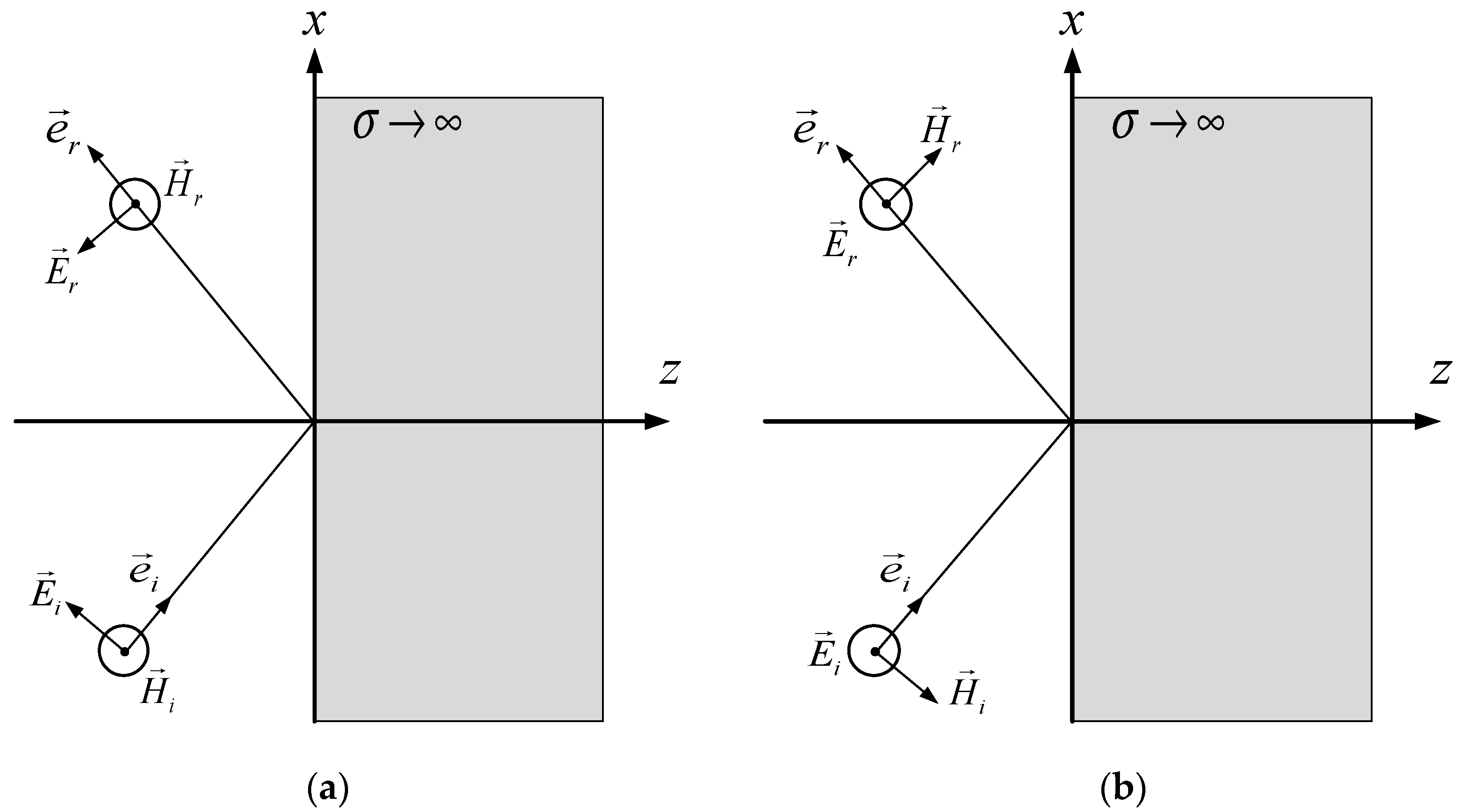
2. Polarization of Electromagnetic Wave
3. Array Optimization for 1-D MAS
4. Array Optimization for 2-D MAS
- (1)
- The coordinates of each antenna along two dimensions are even multiples of 0.5.
- (2)
- The coordinates of each antenna along two dimensions are odd multiples of 0.5.
- (3)
- The coordinate of each antenna along one dimension is an even multiple of 0.5, and along the other dimension is an odd multiple of 0.5.
- 1
- The first case
- 2
- The second case
- 3
- The third case
5. Conclusions
Author Contributions
Funding
Conflicts of Interest
References
- Ulaby, F.; Long, D.G. Microwave Radar and Radiometric Remote Sensing; University of Michigan Press: Ann Arbor, MI, USA, 2014. [Google Scholar]
- Li, Y.; Liu, H.; Zhang, A. End-to-End Simulation of WCOM IMI Sea Surface Salinity Retrieval. Remote Sens. 2019, 11, 217. [Google Scholar] [CrossRef]
- Kilic, L.; Prigent, C.; Aires, F.; Heygster, G.; Pellet, V.; Jimenez, C. Ice Concentration Retrieval from the Analysis of Microwaves: A New Methodology Designed for the Copernicus Imaging Microwave Radiometer. Remote Sens. 2020, 12, 1060. [Google Scholar] [CrossRef]
- Kerr, Y.H.; Waldteufel, P.; Wigneron, J.P.; Martinuzzi, J.A.M.J.; Font, J.; Berger, M. Soil moisture retrieval from space: The Soil Moisture and Ocean Salinity (SMOS) mission. IEEE Trans. Geosci. Remote Sens. 2001, 39, 1729–1735. [Google Scholar] [CrossRef]
- Piepmeier, J.R.; Focardi, P.; Horgan, K.A.; Knuble, J.; Ehsan, N.; Lucey, J. SMAP L-band microwave radiometer: Instrument design and first year on orbit. IEEE Trans. Geosci. Remote Sens. 2017, 55, 1954–1966. [Google Scholar] [CrossRef] [PubMed]
- Tanner, A.B.; Wilson, W.J.; Lambrigsten, B.H.; Dinardo, S.J.S.; Brown, T.; Kangaslahti, P.P.; Gaier, T.C.; Ruf, C.S.; Gross, S.M.; Lim, B.H.; et al. Initial results of the geostationary synthetic thinned array radiometer (GeoSTAR) demonstrator instrument. IEEE Trans. Geosci. Remote Sens. 2007, 45, 1947–1957. [Google Scholar] [CrossRef]
- Ruf, C.S.; Swift, C.T.; Tanner, A.B.; Le Vine, D.M. Interferometric synthetic aperture radiometry for the remote sensing of the Earth. IEEE Trans. Geosci. Remote Sens. 1988, 26, 597–611. [Google Scholar] [CrossRef]
- Xiao, C.; Wang, X.; Dou, H.; Li, H.; Lv, R.; Wu, Y.; Song, G.; Wang, W.; Zhai, R. Non-Uniform Synthetic Aperture Radiometer Image Reconstruction Based on Deep Convolutional Neural Network. Remote Sens. 2022, 14, 2359. [Google Scholar] [CrossRef]
- Chen, L.; Li, Q.; Yi, G.; Zhu, Y. One-dimensional mirrored interferometric aperture synthesis: Performances, simulation, and experiments. IEEE Trans. Geosci. Remote Sens. 2013, 51, 2960–2968. [Google Scholar] [CrossRef]
- Xiao, C.; Li, Q.; Lei, Z.; Zhao, G.; Chen, Z.; Huang, Y. Image Reconstruction with Deep CNN for Mirrored Aperture Synthesis. IEEE Trans. Geosci. Remote Sens. 2022, 60, 5303411. [Google Scholar] [CrossRef]
- Lei, Z.; Dou, H.; Li, Q.; Li, H.; Chen, L.; Chen, K.; Gui, L.; Zhao, G.; Chen, Z.; Xiao, C.; et al. 2-D Mirrored Aperture Synthesis with Four Tilted Planar Reflectors. IEEE Trans. Geosci. Remote Sens. 2022, 60, 2004213. [Google Scholar] [CrossRef]
- Dou, H.; Gui, L.; Li, Q.; Chen, L.; Bi, X.; Wu, Y.; Lei, Z.; Li, Y.; Chen, K.; Lang, L.; et al. Initial results of microwave radiometric imaging with mirrored aperture synthesis. IEEE Trans. Geosci. Remote Sens. 2019, 57, 8105–8117. [Google Scholar] [CrossRef]
- Dong, J.; Li, Q.; Jin, R.; Zhu, Y.; Huang, Q.; Gui, L. A Method for Seeking Low-Redundancy Large Linear Arrays for Aperture Synthesis Microwave Radiometers. IEEE Trans. Antennas Propagat. 2010, 58, 1913–1921. [Google Scholar] [CrossRef]
- Dong, J.; Li, Q.; Shi, R.; Gui, L.; Guo, W. The Placement of Antenna Elements in Aperture Synthesis Microwave Radiometers for Optimum Radiometric Sensitivity. IEEE Trans. Antennas Propagat. 2011, 59, 4103–4114. [Google Scholar] [CrossRef]
- Camps, A.; Cardama, A.; Infantes, D. Synthesis of large low-redundancy linear arrays. IEEE Trans. Antennas Propagat. 2001, 49, 1881–1883. [Google Scholar] [CrossRef]
- Ruf, C.S. Numerical annealing of low-redundancy linear arrays. IEEE Trans. Antennas Propagat. 1993, 41, 85–90. [Google Scholar] [CrossRef]
- Chen, L.; Rao, Z.; Wang, Y.; Zhou, H. The Maximum Rank of the Transfer Matrix in 1-D Mirrored Interferometric Aperture Synthesis. IEEE Geosci. Remote Sens. Lett. 2017, 14, 1580–1583. [Google Scholar] [CrossRef]
- Dou, H.; Chen, K.; Li, Q.; Jin, R.; Wu, Y.; Lei, Z. Analysis and Correction of the Rank-Deficient Error for 2-D Mirrored Aperture Synthesis. IEEE Trans. Geosci. Remote Sens. 2021, 59, 2222–2230. [Google Scholar] [CrossRef]
- Yi, G.; Hu, F.; Jin, R.; Li, D.; Yang, H.; Dong, J. Array configuration design of 1-D mirrored interferometric aperture synthesis. IEEE Geosci. Remote Sens. Lett. 2012, 9, 1021–1025. [Google Scholar] [CrossRef]
- Dou, H.; Chen, K.; Li, Q.; Wu, Y.; Lei, Z. Maximum-Rank Arrays for Two-Dimensional Mirrored Aperture Synthesis. IEEE Geosci. Remote Sens. Lett. 2021, 18, 499–503. [Google Scholar] [CrossRef]
- Lei, Z.; Chen, L.; Li, Q.; Dou, H.; Chen, K. Rank-Full Arrays for 2-D Mirrored Aperture Synthesis. IEEE Geosci. Remote Sens. Lett. 2022, 19, 5003305. [Google Scholar]


| N | The Coordinates of the Antennas |
|---|---|
| 5 | 1.5 4.5 6.5 7.5 8.5 |
| 6 | 2 6 9 10 11 12 |
| 7 | 2 6 10 13 14 15 16 |
| 8 | 2.5 7.5 12.5 16.5 17.5 18.5 19.5 20.5 |
| 9 | 2.5 7.5 12.5 17.5 21.5 22.5 23.5 24.5 25.5 |
| 10 | 3 9 15 21 26 27 28 29 30 31 |
| 11 | 3.5 10.5 17.5 24.5 27.5 31.5 32.5 33.5 35.5 36.5 37.5 |
| 12 | 3.5 10.5 17.5 24.5 31.5 37.5 38.5 39.5 40.5 41.5 42.5 43.5 |
| 13 | 3.5 10.5 17.5 23.5 30.5 37.5 43.5 44.5 45.5 46.5 47.5 48.5 49.5 |
| 14 | 3.5, 10.5, 17.5, 24.5, 31.5, 38.5, 44.5, 50.5, 51.5, 52.5, 53.5, 54.5, 55.5, 56.5 |
| N | MRA | DPA | ||
|---|---|---|---|---|
| Maximum Baseline | Rank | Maximum Baseline | Rank | |
| 5 | 11 | 9 | 16 | 16 |
| 6 | 17 | 15 | 23 | 23 |
| 7 | 22 | 21 | 31 | 31 |
| 8 | 29 | 27 | 40 | 40 |
| 9 | 37 | 35 | 50 | 50 |
| 10 | 46 | 45 | 61 | 61 |
| 11 | 57 | 55 | 74 | 74 |
| 12 | 64 | 63 | 86 | 86 |
| 13 | 72 | 71 | 98 | 98 |
| 14 | 80 | 79 | 112 | 112 |
| The size of the array | 3 × 3 | 3 × 4 | 3 × 5 | 3 × 6 |
| The rank of P | 40 | 55 | 69 | 83 |
| The size of the array | 4 × 3 | 4 × 4 | 4 × 5 | 4 × 6 |
| The rank of P | 55 | 73 | 91 | 109 |
| The size of the array | 5 × 3 | 5 × 4 | 5 × 5 | 5 × 6 |
| The rank of P | 69 | 91 | 113 | 135 |
| The size of the array | 6 × 3 | 6 × 4 | 6 × 5 | 6 × 6 |
| The rank of P | 83 | 109 | 135 | 161 |
| The size of the array | 2.5 × 2.5 | 2.5 × 3.5 | 2.5 × 4.5 | 2.5 × 5.5 |
| The rank of P | 30 | 42 | 54 | 66 |
| The size of the array | 3.5 × 2.5 | 3.5 × 3.5 | 3.5 × 4.5 | 3.5 × 5.5 |
| The rank of P | 42 | 58 | 74 | 90 |
| The size of the array | 4.5 × 2.5 | 4.5 × 3.5 | 4.5 × 4.5 | 4.5 × 5.5 |
| The rank of P | 54 | 74 | 94 | 114 |
| The size of the array | 5.5 × 2.5 | 5.5 × 3.5 | 5.5 × 4.5 | 5.5 × 5.5 |
| The rank of P | 66 | 90 | 114 | 138 |
| The size of the array | 2.5 × 3 | 2.5 × 4 | 2.5 × 5 | 2.5 × 6 |
| The rank of P | 35 | 48 | 60 | 72 |
| The size of the array | 3.5 × 3 | 3.5 × 4 | 3.5 × 5 | 3.5 × 6 |
| The rank of P | 49 | 66 | 82 | 98 |
| The size of the array | 4.5 × 3 | 4.5 × 4 | 4.5 × 5 | 4.5 × 6 |
| The rank of P | 63 | 84 | 104 | 124 |
| The size of the array | 5.5 × 3 | 5.5×4 | 5.5 × 5 | 5.5 × 6 |
| The rank of P | 77 | 102 | 126 | 150 |
| The Shape of the Array | N | RMSE (K) | The Size of P | The Rank of P |
|---|---|---|---|---|
| Rectangular | 22 | 5.3 | 231 × 178 | 145 |
| L-shaped | 22 | 1.39 | 462 × 252 | 250 |
Disclaimer/Publisher’s Note: The statements, opinions and data contained in all publications are solely those of the individual author(s) and contributor(s) and not of MDPI and/or the editor(s). MDPI and/or the editor(s) disclaim responsibility for any injury to people or property resulting from any ideas, methods, instructions or products referred to in the content. |
© 2022 by the authors. Licensee MDPI, Basel, Switzerland. This article is an open access article distributed under the terms and conditions of the Creative Commons Attribution (CC BY) license (https://creativecommons.org/licenses/by/4.0/).
Share and Cite
Li, H.; Li, G.; Dou, H.; Xiao, C.; Lei, Z.; Lv, R.; Li, Y.; Wu, Y.; Song, G. Array Configuration Design for Mirrored Aperture Synthesis Radiometers Based on Dual-Polarization Measurements. Remote Sens. 2023, 15, 167. https://doi.org/10.3390/rs15010167
Li H, Li G, Dou H, Xiao C, Lei Z, Lv R, Li Y, Wu Y, Song G. Array Configuration Design for Mirrored Aperture Synthesis Radiometers Based on Dual-Polarization Measurements. Remote Sensing. 2023; 15(1):167. https://doi.org/10.3390/rs15010167
Chicago/Turabian StyleLi, Hao, Gang Li, Haofeng Dou, Chengwang Xiao, Zhenyu Lei, Rongchuan Lv, Yinan Li, Yuanchao Wu, and Guangnan Song. 2023. "Array Configuration Design for Mirrored Aperture Synthesis Radiometers Based on Dual-Polarization Measurements" Remote Sensing 15, no. 1: 167. https://doi.org/10.3390/rs15010167
APA StyleLi, H., Li, G., Dou, H., Xiao, C., Lei, Z., Lv, R., Li, Y., Wu, Y., & Song, G. (2023). Array Configuration Design for Mirrored Aperture Synthesis Radiometers Based on Dual-Polarization Measurements. Remote Sensing, 15(1), 167. https://doi.org/10.3390/rs15010167