Abstract
For safety-of-life applications used together with global navigation satellite systems, such as in civil aviation and autonomous driving, integrity is of paramount importance. Integrity monitoring protects the user safety based on two general approaches: mitigating large signal failures and bounding the residual errors. The fault detection and exclusion (FDE) of faulty satellites is part of the former approach. In the classical integrity monitoring algorithms in civil aviation, the use of test statistics based on least squares residuals relies on the assumption that the observations from different satellites are independent. When applied to urban environments with spatial correlation introduced by large multipath errors, a review of the FDE method is needed. With the optimal FDE method defined as the one with minimized integrity risk, we propose two optimization criteria for use in fault detection and fault exclusion. The optimal test statistics were obtained by analytical derivation for cases with and without correlations among different satellites. This method was theoretically compared with another commonly used test statistic using the minimum detectable bias, and it was numerically compared using the horizontal protection level under the scenario of advanced receiver autonomous integrity monitoring. The optimal test produces less conservative protection level results, and its advantage is especially obvious when the geometries are weak, or when the correlation coefficients among the satellites are high.
1. Introduction
Global navigation satellite systems (GNSSs) may contain various forms of signal failures (e.g., ionosphere anomalies, satellite clock and ephemeris failures, signal deformation, etc.). The integrity is a measure of the trust that can be placed in the correctness of the information supplied by a navigation system, including the ability of the system to provide timely warnings about when it should not be used. For safety-of-life applications, such as civil aviation [1] and intelligent transport systems (ITSs) [2,3], the integrity is of paramount importance. In civil aviation, different integrity monitoring systems are available for different flight phases, including receiver autonomous integrity monitoring (RAIM), space-based augmentation systems (SBASs), and ground-based augmentation systems (GBASs). The required integrity risk or probability of hazardously misleading information (PHMI) must not exceed 10−7/h for enroute users with RAIM and the SBAS, and it must not exceed 10−7/150 s for precision approach users with the SBAS and GBAS [1]. For ITSs, the safety integrity level four, with a tolerable hazard rate, must not exceed 10−9/h for railway navigation [4], and an integrity requirement of 10−8/h has been preliminary derived for autonomous vehicles [5].
The general purpose of integrity monitoring is to mitigate large faults and bound residual errors within a confidence level. For example, in RAIM, after fault detection and exclusion (FDE), the undetected position errors are bounded by the protection level (PL) within a required integrity risk [6]. If the PL exceeds an alert limit, the navigation service is considered unavailable. RAIM FDE is performed via a consistency check based on the redundancy in the measurements using least squares residuals [7]. In the GBAS and SBAS, although the integrity monitoring scheme becomes more complicated, a basic RAIM FDE function is still needed. For example, a consistency check based on least squares residuals is conducted on the satellite clock fault when computing the user differential range error in the SBAS [8], and this has been used as one of the options to accomplish the integrity monitoring function in ITSs [9].
Compared with the least squares estimator using the Gauss–Markov model in civil aviation, the main navigation solution in ITSs is mostly based on the Kalman filter using the first-order Gauss–Markov model [10]. The previous FDE method based on least squares residuals no longer performs as well as that based on the Kalman filter. For example, the slowly growing errors can be assimilated and may not be reflected in the innovations. Moreover, an undetected satellite fault of the previous epoch maintains its impact on the current epoch estimation. Therefore, a basic RAIM FDE function using least squares residuals is often implemented with the Kalman filter to exclude the faulty satellite from further processing [10,11].
In the classical integrity monitoring techniques in civil aviation, the observations from different satellites are assumed to be independent [1]. With the use of these techniques for ITSs, the multipath-introduced spatial correlations among different satellites become nonnegligible [12]. Although the FDE function under the scenario of integrity monitoring in civil aviation is mature, it may no longer be an optimal method for ITSs. Therefore, the optimality of the classical RAIM FDE method was reviewed and evaluated for cases both with and without correlation.
The optimal FDE method is defined as the one with a minimized PHMI, or equivalently, a less conservative PL. Recently, a new FDE estimator for minimizing the PL was proposed [13] in which the spatial correlation is not considered. In this paper, two new optimization criteria were designed from a deterministic perspective for either fault detection or fault exclusion. Based on the analytical derivations, explicit conclusions on formulating the test statistics were obtained for cases both with and without correlation.
The rest of this paper is organized as follows. First, the basic model is defined in the parity space using the least square estimator. Next, the optimal test statistics are derived based on the optimization criteria for both fault detection and fault exclusion. Then, the PL calculation is extended for the optimal method and illustrated with a numerical example. Finally, the main conclusions are drawn.
2. Basic Model
Without a loss of generality, a basic GNSS observation model can be assumed for either civil aviation or ITSs with different positioning modes:
where is the observation vector, which can be the undifferenced pseudorange observation for single-point positioning in ARAIM, the double-differenced carrier phase observation in real-time kinematic (RTK) positioning, or the undifferenced carrier phase observation for precise point positioning (PPP); is the unknown state vector; m is the number of visible satellites; n is the number of unknown parameters; is the design matrix; is the residual error, which is assumed to follow the Gaussian distribution with the zero mean and covariance matrix of the .
With dual-frequency and multi-constellation signals available in civil aviation, RAIM is evolving toward advanced RAIM (ARAIM) [6]. In both the RAIM and ARAIM algorithms, the off-diagonal elements in the are assumed to be zeros without correlations among different satellites. To bind the standard deviation for each observation with each diagonal element, different errors are individually bounded according to the established error models (e.g., satellite clock and orbit errors, ionosphere errors for single-frequency users, troposphere errors, multipaths, and noise). The squared sum of the standard deviation for each error is used as the variance of each observation [6].
For urban environments, the off-diagonal elements in the can be nonzero values with large multipath errors [12], which can be bounded using a machine learning method [14]. Further study is needed to bound both the off-diagonal and diagonal elements in , which is not within the scope of this paper. With the assumed to be given, the following derivatives and conclusions are not affected by its specific values. To be applicable in both civil aviation and ITSs, two cases of the are considered: (1) with correlation, and (2) without correlation.
The parity space is defined as an orthogonal space relative to the observation space. The purpose of using the parity space is to simplify the derivation process. A general parity matrix is defined as , with two conditions satisfied: and , where represents a unit vector with zeros in all positions except for the ith position, which has a value of one, indicating the location of a single-satellite fault. The general parity vector is used to define a scalar :
The general form of a test statistic under the faulty hypothesis () with standard normal distribution is defined as:
There are multiple choices of that satisfy the two conditions, and an optimal parity matrix is derived as follows to achieve an optimal FDE performance.
3. Optimal Fault Detection and Exclusion
Considering the case of horizontal positioning, the integrity risk () is defined under the faulty hypothesis () for which the ith satellite is faulty:
where is the horizontal positioning error; is the horizontal protection level (HPL); is the test threshold, which, with the test statistics () of a standard normal distribution, can be determined by a given probability of false alarm (PFA) under the fault-free hypothesis; is the prior probability of hypothesis , and the sum of the prior probabilities of the fault-free and all faulty hypotheses is 1; is independent of the , with a least squares estimator using either residual-based test statistics or statistics based on solution separation. The two types of test statistics are equivalent [7]. The method based on residual-based test statistics is used as the example in this paper. Because and are independent, and are two independent probabilities. Therefore, the integrity risk is expressed as a multiplication of three separate probabilities: . With given beforehand, if is minimized separately, then the totally integrity risk can be reduced. Therefore, an optimal FDE test is one with minimized risk of , which is related to the probability of missed detection (PMD).
In the current test procedures, if the maximum test statistic exceeds a predefined threshold, then the corresponding satellite is regarded as faulty. Therefore, optimizing the fault detection performance is equivalent to maximizing the sensitivity of the test statistics with regard to the faults and minimizing the sensitivity of the test statistics to other errors. In this way, a small enough fault can trigger an alarm, and the effects of unavoidable random errors can be suppressed to minimize the PMD. If the fault exclusion performance is also optimized by maximizing the fault from satellite i in the , the continuity risk can benefit from it [15]. Therefore, two criteria are defined to optimize the fault detection and fault exclusion from a deterministic perspective: (a) the maximization of the expectation of the under hypothesis in the presence of other random errors among the multiple choices of ; (b) the maximum expectation of all the test statistics needs to be under hypothesis . The criteria (a and b) are further expressed by Equations (5) and (6), respectively:
3.1. Optimal Fault Detection
To obtain an optimal parity matrix under criterion a, the following proof is provided. Assuming the standard parity matrix () is the orthonormal basis of the left null space of (i.e., and ), is expressed as a linear combination of the with as a coefficient vector:
An optimal can be obtained by using the square of criterion a, which can be expressed as:
where , and is the magnitude of a fault on satellite (i). With as a symmetric positive definite, the maximum value is obtained with the following condition based on the Cauchy–Schwarz inequality [16]:
where is an arbitrary nonzero real number. Therefore, for a given size of a single fault, is maximum when the optimal parity vector () is used at :
The corresponding optimal test statistic for fault detection is given by:
Another test statistic based on least square residuals is denoted as the v-test [11,17]:
where is the least square residual, and is the covariance matrix of the . The is equivalent to the only when there is no correlation in the . Therefore, the is an optimal choice for fault detection both with and without correlation, while the can be used only for independent observations to maintain the optimal fault detection performance.
3.2. Optimal Fault Exclusion
For the FDE, the necessity to include fault exclusion was examined, and it was concluded that airborne exclusion is required to meet the enroute continuity risk of the H-ARAIM [15]. Similarly, fault exclusion is needed to improve the service continuity in ITSs. The optimal test statistics for fault exclusion under criterion b are derived from the following:
Criterion b can be met if the in (2) is a symmetric semipositive definite:
For a symmetric semipositive definite (), the diagonal entries () are real and nonnegative. Assuming the deterministic fault is , where is the magnitude of the fault size on satellite i, then:
Because is symmetric semipositive, the following inequality can be obtained:
In other words, for any , it holds that:
Therefore, can also satisfy criterion b, which is an optimal choice for fault exclusion with or without correlation. is only an optimal choice for fault exclusion if there is no correlation between the observations.
4. Protection Level
Instead of calculating the integrity risk, the HPL is computed as the position error bound within a required integrity risk. Generally, there are two types of RAIM methods: the classical method and multiple-hypothesis solution separation method [18]. With the classical method, the random positioning error is bound by the HPL under the fault-free hypothesis () within an allocated integrity risk:
where is the allocated integrity risk under , is the prior probability of hypothesis , and is the standard deviation of the horizontal position error. The HPL under the faulty hypothesis is designed to bind the positioning error by two terms separately: the bias and random error. The bias term is used to bind the undetected error from the statistical test. For a given standard deviation of test statistics, a non-centrality parameter of the test statistics () can be bound by the PFA allocated from the continuity risk and the PMD allocated from the integrity risk. The MDB is then defined by transferring the from the test statistic domain to the range domain. Therefore, the MDB represents the magnitude of a fault in an observation, which can be detected under given PFAs and PMDs. The MDBs of the optimal test and v-test can be expressed by both the parity space and least squares residuals, respectively, using [17]:
With the bias term bounded, the remaining random errors need to satisfy the allocated integrity risk. The classical HPL under hypothesis can be defined by:
where , with is the number of visible satellites; is the horizontal projection matrix from the range domain to the position domain for satellite i; is the inverse of the cumulative distribution function with standard normal distribution; is the allocated integrity risk for hypothesis ; is the prior probability of hypothesis . The final HPL is the maximum one among all the hypotheses.
Therefore, if different FDE test statistics are selected, then their differences in the HPL formula relate only to the MDB parameter. As proven in Appendix A, the MDB of the optimal test is always equal to or smaller than that of the v-test. It should be noted that the equality holds if and only if there is no correlation among observations. Therefore, the optimal test has a better FDE performance and produces less conservative HPL results than the v-test.
5. Numerical Results
To further demonstrate the performances of the classical HPL with different FDE methods, 24 h data were used to obtain the numerical results. The user’s static position was set as 22.3042°N and 114.1798°E at Hong Kong Polytechnic University. The GPS almanac data on 27 November 2022 with 32 satellites was used to calculate the satellite position under a one-minute sampling interval. Given the user and satellite positions, the elevation angle was then computed, which was used to formulate the matrices of , , , and . The mask angle was set to 5°. The total required integrity risk was 10−7, which was evenly distributed among the fault-free and faulty hypotheses. The prior probability of each faulty hypothesis () was 1 × 10⁻⁴. The PFA and PMD of each hypothesis were 3.33 × 10⁻⁷ and 10−3, respectively [18]. The observation errors from each satellite were assumed to follow a standard normal distribution with a correlation existing between two satellites. Two examples with correlation coefficients of 0.2 and 0.9 are illustrated in Figure 1 and Figure 2, respectively, with the classical HPL method based on the optimal test and v-test.
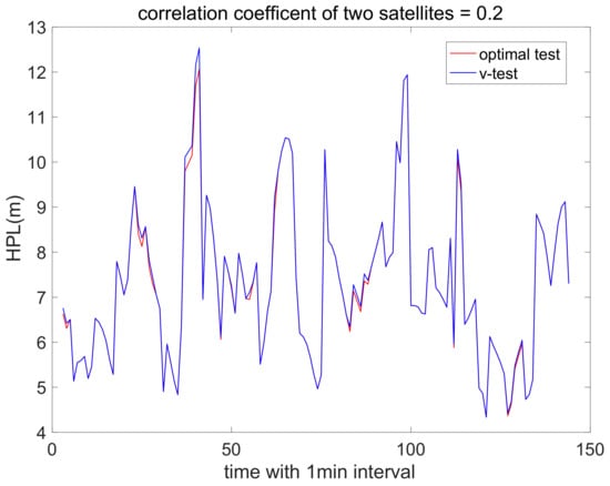
Figure 1.
Classical HPL under optimal test and v-test with low correlation.
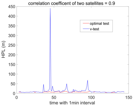
Figure 2.
Classical HPL under optimal test and v-test with high correlation.
Comparing Figure 1 and Figure 2, the optimal test maintains low HPL values in both the low- and high-correlation cases, while the v-test generates high HPL values in the high-correlation cases with reduced service availability. The high peaks in both Figure 1 and Figure 2 occur simultaneously, which indicates that the v-test amplifies the weak geometry under the spatial correlation in the HPL. Therefore, the optimal test is feasible for scenarios both with and without spatial correlation among the observations, while the v-test can only be used for cases in which there is little correlation.
6. Conclusions
The conventional RAIM FDE method was developed based on the assumption that the observations from different satellites are independent. To apply this method to other safety-of-life applications (e.g., ITSs) with spatial correlation among the observations, the design of the test statistics was reviewed. The optimal test statistics are defined as those that minimize the integrity risk, and the optimal solution is derived from a deterministic perspective. It was valid for cases both with and without correlation without a loss of generality. To further validate this conclusion, the MDBs of the optimal test statistics and those of another commonly used statistic were compared. It was theoretically demonstrated that the optimal test always generates smaller MDBs than the alternative method with correlation. Smaller MDBs indicate an enhanced FDE performance and less conservative HPL results, which is equivalent to a minimized integrity risk. This conclusion was also demonstrated with numerical results with 24 h GPS data. The HPL results with the optimal test were lower than those with the alternative test, which was especially obvious with high correlation coefficients and weak geometries. With its proven optimality, the FDE method can be used in integrity monitoring for both civil aviation and ITSs with improved service availability. Further research is planned for binding the observation error with spatial correlation for urban environments.
Funding
This research was funded by the National Natural Science Foundation of China grant number 42004029 and the University Grants Committee/Research Grants Council grant number 25202520).
Conflicts of Interest
The author declares no conflict of interest.
Appendix A. Comparison of Two MDBs
First, , , and are expressed as block matrices:
where , , , and .
where , and .
The following derivations can then be obtained:
The MDBs in (19) and (20) can be written as (A9) and (A10), respectively:
Therefore, based on the above two terms, to compare the values of and , the values of and should first be compared. The difference between these two terms is given by:
Under the Schur complement, because the is symmetric, positive, and semidefinite, the is positive definite, and is positive semidefinite. The following derivations are therefore obtained:
The condition of is also obtained as follows:
Therefore, when , which is equivalent to the case when the or is a diagonal square matrix for any i, it holds that . Moreover, when is a diagonal matrix, then . Therefore, the relationship of both the necessity and sufficiency is obtained:
References
- Annex-10. Aeronautical Telecommunications—Radio Navigation Aids, 7th ed.; International Civil Aviation Organization (ICAO): Montreal, QC, Canada, 2018; Volume 1. [Google Scholar]
- Tijero, E.D.; Fernández, L.M.; Zarzosa, J.I.H.; García, J.; Ibañez-Guzmán, J.; Stawiarski, E.; Xu, P.; Avellone, G.; Pisoni, F.; Falletti, E.; et al. High Accuracy Positioning Engine with an Integrity Layer for Safety Autonomous Vehicles. In Proceedings of the ION GNSS+ 2018, Institute of Navigation, Miami, FL, USA, 24–28 September 2018; pp. 1566–1572. [Google Scholar]
- Zhu, N.; Marais, J.; Bétaille, D.; Berbineau, M. GNSS Position Integrity in Urban Environments: A Review of Literature. IEEE Trans. Intell. Transp. Syst. 2018, 19, 2762–2778. [Google Scholar] [CrossRef]
- Neri, A.; Rispoli, F.; Salvatori, P.; Vegni, A.M. A Train Integrity Solution Based on GNSS Double-Difference Approach. In Proceedings of the ION GNSS+ 2014, Institute of Navigation, Tampa, FL, USA, 8–12 September 2014; pp. 34–50. [Google Scholar]
- Reid, T.G.R.; Houts, S.E.; Cammarata, R.; Mills, G.; Agarwal, S.; Vora, A.; Pandey, G. Localization requirements for autonomous vehicles. SAE J. Connect. Autom. Veh. 2019, 2, 173–190. [Google Scholar] [CrossRef]
- ARAIM; EU-U.S. Cooperation on Satellite Navigation Working Group C-ARAIM Technical Subgroup. 2016. Available online: https://www.gps.gov/policy/cooperation/europe/2016/working-group-c/ARAIM-milestone-3-report.pdf (accessed on 25 December 2022).
- Joerger, M.; Pervan, B. Fault detection and exclusion using solution separation and chi-squared ARAIM. IEEE Trans. Aerosp. Electron. Syst. 2016, 52, 726–742. [Google Scholar] [CrossRef]
- Tsai, Y.J. Wide-Area Differential Operation of the Global Positioning System: Ephemeris and Clock Algorithms. Ph.D. Thesis, Stanford University, Stanford, CA, USA, 1999. [Google Scholar]
- Wang, K.; El-Mowafy, A.; Rizos, C.; Wang, J. SBAS DFMC service for road transport: Positioning and integrity monitoring with a new weighting model. J. Geod. 2021, 95, 29. [Google Scholar] [CrossRef]
- El-Mowafy, A.; Kubo, N. Integrity monitoring for positioning of intelligent transport systems using integrated RTK-GNSS, IMU and vehicle odometer. IET Intell. Transp. Syst. 2018, 12, 901–908. [Google Scholar] [CrossRef]
- Bahadur, B.; Nohutcu, M. PPPH: A MATLAB-based software for multi-GNSS precise point positioning analysis. GPS Solut. 2018, 22, 113. [Google Scholar] [CrossRef]
- Zhang, G.; Icking, L.; Hsu, L.; Schön, S. A Study on Multipath Spatial Correlation for GNSS Collaborative Positioning. In Proceedings of the 34th International Technical Meeting of the Satellite Division of the Institute of Navigation (ION GNSS+ 2021), St. Louis, MO, USA, 20–24 September 2021; pp. 2430–2444. [Google Scholar]
- Blanch, J.; Walter, T. A Fault Detection and Exclusion Estimator Designed for Integrity. In Proceedings of the 34th International Technical Meeting of the Satellite Division of the Institute of Navigation, St. Louis, MO, USA, 20–24 September 2021. [Google Scholar]
- No, H.; Milner, C. Machine Learning Based Overbound Modeling of Multipath Error for Safety Critical Urban Environment. In Proceedings of the ITM, Institute of Navigation, St. Louis, MO, USA, 20–24 September 2021; pp. 180–194. [Google Scholar]
- Zhai, Y.; Joerger, M.; Pervan, B. Fault Exclusion in Multi-Constellation Global Navigation Satellite Systems. J. Navig. 2018, 71, 1281–1298. [Google Scholar] [CrossRef]
- Jin, H.; Zhang, H. Optimal parity vector sensitive to designated sensor fault. IEEE Trans. Aerosp. Electron. Syst. 1999, 35, 1122–1128. [Google Scholar]
- Teunissen, P.J.G. Quality Control and GPS. In GPS for Geodesy; Springer: Berlin/Heidelberg, Germany, 1998. [Google Scholar]
- Jiang, Y.; Wang, J. A new approach to calculate the Horizontal Protection Level. J. Navig. 2014, 69, 57–74. [Google Scholar] [CrossRef]


Disclaimer/Publisher’s Note: The statements, opinions and data contained in all publications are solely those of the individual author(s) and contributor(s) and not of MDPI and/or the editor(s). MDPI and/or the editor(s) disclaim responsibility for any injury to people or property resulting from any ideas, methods, instructions or products referred to in the content. |
© 2022 by the author. Licensee MDPI, Basel, Switzerland. This article is an open access article distributed under the terms and conditions of the Creative Commons Attribution (CC BY) license (https://creativecommons.org/licenses/by/4.0/).