Article

Applying Variable Selection Methods and Preprocessing Techniques to Hyperspectral Reflectance Data to Estimate Tea Cultivar Chlorophyll Content

1
Faculty of Agriculture, Shizuoka University, Shizuoka 422-8529, Japan
2
Institute for Tea Science, Shizuoka University, Shizuoka 422-8529, Japan
3
Institute of Fruit Tree and Tea Science, National Agriculture and Food Research Organization, Shimada 428-8501, Japan
*
Author to whom correspondence should be addressed.
Remote Sens. 2023, 15(1), 19; https://doi.org/10.3390/rs15010019
Submission received: 14 November 2022 / Revised: 14 December 2022 / Accepted: 18 December 2022 / Published: 21 December 2022
(This article belongs to the Special Issue Remote Sensing for Estimating Leaf Chlorophyll Content in Plants)

Abstract

:
Tea is second only to water as the world’s most popular drink and it is consumed in various forms, such as black and green teas. A range of cultivars has therefore been developed in response to customer preferences. In Japan, farmers may grow several cultivars to produce different types of tea. Leaf chlorophyll content is affected by disease, nutrition, and environmental factors. It also affects the color of the dried tea leaves: a higher chlorophyll content improves their appearance. The ability to quantify chlorophyll content would therefore facilitate improved tea tree management. Here, we measured the hyperspectral reflectance of 38 cultivars using a compact spectrometer. We also compared various combinations of preprocessing techniques and 14 variable selection methods. According to the ratio of performance to deviation (RPD), detrending was effective at reducing the influence of additive interference of scattered light from particles and then regression coefficients was the best variable selection method for estimating the chlorophyll content of tea leaves, achieving an RPD of 2.60 and a root mean square error of 3.21 μg cm−2.

1. Introduction

Green tea, which is produced from unfermented tea leaves, is widely consumed in East Asia. Some green tea cultivars have been developed to enhance pest resistance, improve quality, and increase yield. Black tea is also produced, in response to the high demand for black tea on the global market. Further, hybrids of a Chinese black tea and Assam, which is from India, such as Benifuuki, have been cultivated and are occasionally introduced as high-grade Japanese black teas [1]. Some farmers cultivate several cultivars in their tea fields, but they may differ in harvesting season, stress tolerance, and quality characteristics [2], making management complex.
Leaf chlorophyll content influences a plant’s light-response curve under low stress conditions and has been used as the main indicator for estimating photosynthetic ability, health status, and resistance to a wide range of diseases [3,4]. Chlorophyll content also provides information regarding crops’ nitrogen levels, which play a major role in yield and quality [5]. Further, chlorophyll content is a good indicator of tea quality, since it is strongly related to the color of the dried tea leaves [6] and the flavor of tea is principally determined by its chemical components. Chlorophyll content is thus positively correlated with the total quality score of a tea, as well as its scores for appearance and the infused leaf [7].
Spectrophotometric methods using ultraviolet and visible (UV–VIS) spectroscopy or high-performance liquid chromatography (HPLC) are often used to measure chlorophyll content precisely [8,9]. However, these techniques are expensive, labor-intensive, and occasionally unsuitable for in situ measurements. Conventional chlorophyll meters, such as the SPAD-502 Leaf Chlorophyll Meter (Konica Minolta, Tokyo, Japan), have been used to quantify subtle changes or trends in vegetation [10]. A SPAD value corresponding to the chlorophyll content of the leaf is calculated based on the transmittance of red and infrared radiation through the leaf and then some previous studies have reported variation in leaf thickness affects the relationship between SPAD readings and leaf dry weight, and this relationship can vary among cultivars, developmental stages, and environmental conditions [11,12]. Such variations can confound the interpretation of the data derived from these devices.
Remote sensing based on hyperspectral reflectance has also been used to estimate chlorophyll content, and some authors have proposed methods for simultaneously determining chlorophyll content and other leaf properties [13,14]. Furthermore, machine learning algorithms have been used for evaluating vegetation traits, such as plant drought impact and physiological status, from hyperspectral reflectance [15,16] and identifying cultivars [17]. Therefore, hyperspectral remote sensing can be used as an alternative to traditional tools for estimating chlorophyll contents in tea cultivars. Field-portable spectroradiometers, such as the Ocean Optics hyperspectral Vis–NIR spectroradiometer [18,19] and the Analytical Spectral Devices (ASD) FieldSpec series [20,21,22,23,24,25,26], have been widely used to obtain hyperspectral data. However, the high cost of these devices renders their use infeasible at the consumer level. Developing an affordable hyperspectral remote sensing system would thus be highly beneficial [27]. Sensitive, affordable, and fingertip-sized spectrometers have recently become available and are used for measuring various light levels. To obtain reflectance data, a white reference surface and reflected radiation should be measured under stable conditions; however, this is not possible when using hand-held sensors. Furthermore, the background behind the leaf, such as an observer’s hand, tea petioles, or other leaves, affects the readings. Additionally, some of the light hitting the leaf surface is transmitted through the leaf and may be reflected back by background objects and retransmitted through the leaf, so that the sensor records additional light. Thus, plant probes have been used to standardize measurement conditions [28]. In this study, we used a hyperspectral sensor (colorcompass-LF) developed on a compact spectrometer (C12880MA-10, Hamamatsu Photonics, Shizuoka, Japan) with a leaf clip on a plant probe and evaluated its potential for providing hyperspectral data that can be used to estimate chlorophyll content.
Although vegetation properties can be evaluated using various hyperspectral remote-sensing approaches, variable selection is an important process in generating robust regression models. The underlying principle of variable selection methods is to select a small number of representative variables that then produce more concise and effective spectral data and play important roles in the multivariate analysis, because removing redundant variables is effective for producing better prediction results [29,30]. We therefore compared the performance of 14 variable selection methods combined with six different preprocessing techniques.
Firstly, the utility of reflectance data obtained using a colorcompass-LF was evaluated for estimating chlorophyll content in 38 tea cultivars. Secondly, an effective combination of variable selection methods and preprocessing techniques was identified using the hyperspectral reflectance data acquired with the colorcompass-LF.

2. Materials and Methods

2.1. Measurements

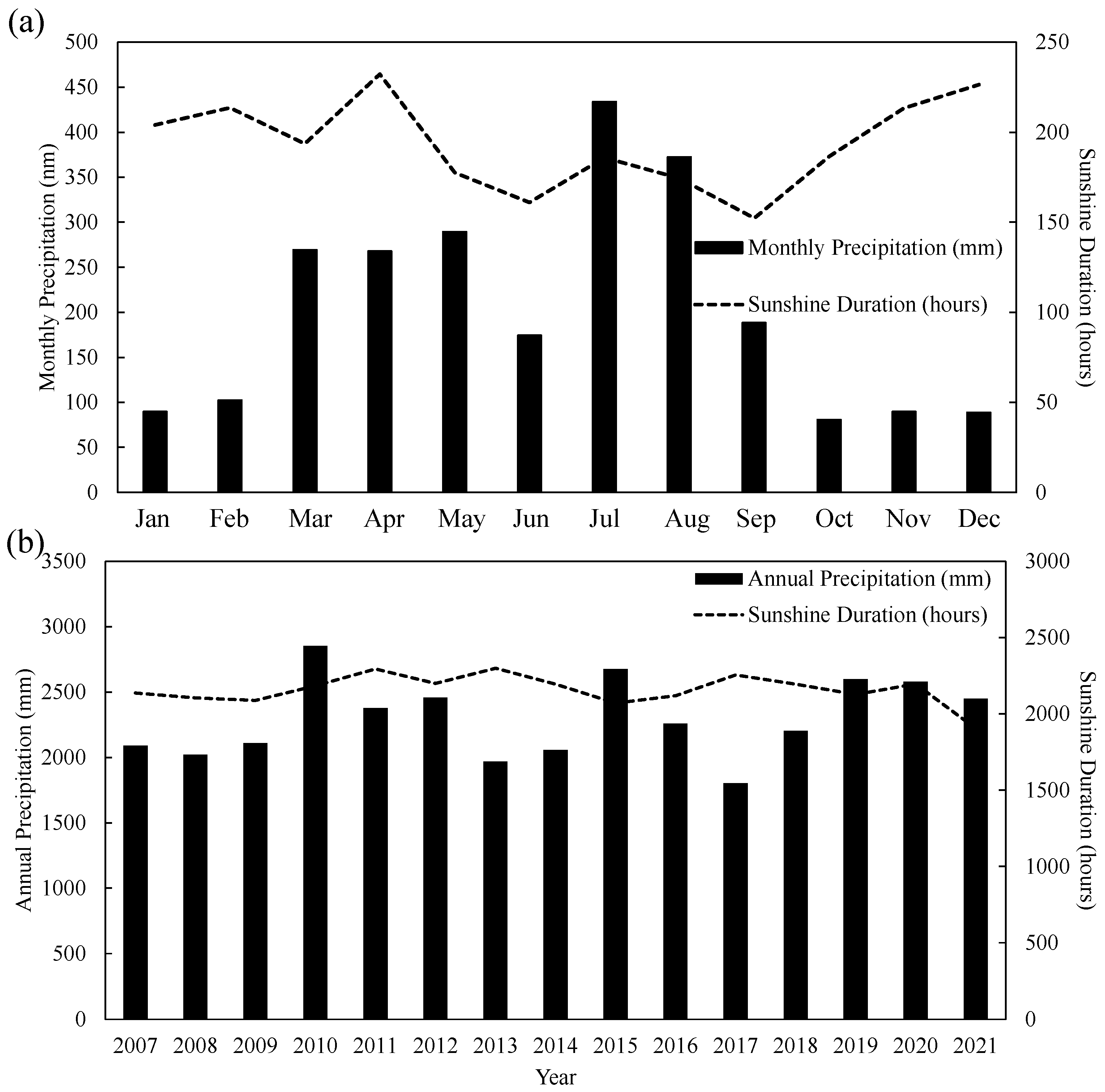
The experiments were conducted at the Institute of Fruit Tree and Tea Science, National Agriculture and Food Research Organization, Shimada, Japan (Figure 1). Daily temperatures and precipitation ranges were 12.5–19.2 °C and 0–17.5 mm, respectively, during the experiment. Figure 2a shows monthly precipitation amounts and monthly sunshine durations in 2021 and Figure 2b shows annual precipitation amounts and annual sunshine durations from 2007 to 2021.
The tea field comprised 39 ridges and a different cultivar was cultivated on each ridge; however, Yabukita and Yutakamidori were cultivated in the two ridges which had no labels in Figure 1. We therefore collected samples from 38 tea cultivars. While most of the cultivars, including Sencha and Matcha, are grown for green tea, Sunrouge (the product of Camellia taliensis × C. sinensis) yields a pink tea, and Benifuuki, Benihikari, and Benihomare produce black tea. Yabukita is the most commonly planted cultivar and provides approximately 85% of Japan’s tea production. Yabukita is commonly produced as Sencha but may also be processed into Matcha. However, this cultivar is susceptible to diseases such as anthracnose and gray blight.
Several cultivars are produced by crossing Yabukita with other cultivars to ensure better pest resistance, quality, and yield of green tea. These include Fukumidori, Harumidori, Hokumei, Kanayamidori, Meiryoku, Minekaori, Okumidori, Ryoufuu, Saemidori, Sayamakaori, Soufuu, and Yumewakaba. The cultivars Fuushun, Saeakari, Sainomidori, Seimei, Harumoegi, Kanaemaru, and Yumekaori are the second filial generation of some of these crosses.
Yabukita, Makinoharawase, and Yaeho were selected from local varieties in the Shizuoka Prefecture, Japan. Asagiri and Asatsuyu were selected from local varieties in the Kyoto Prefecture, and Yutakamidori has the same phylogeny as Asatsuyu. Okuyutaka and Shunmei are crosses of Yutakamidori. Miyamakaori is a cross of Saitama 1, Kyoken 283, and Harunonagomi. Nagomiyutaka is a cross of Saitama 1 and Miyazaki 8. Other crosses are as follows: Minamisayaka (MiyaA-6 × F1NN27), Okuharuka (Saitama 20 × Saitama 7), and Sakimidori (F1NN27 × ME52). Tea nursery stocks were transplanted in 2007–2009. The fertilizer application rates were N-P2O5-K2O = 506-140-208 kg/ha/yr. In these fields, the width between ridges was 0.3 m, and the width of the canopy of tea plants was 1.5 m.
On 10 May, 20 June, and 28 June, we collected 234 samples from the third leaf of the tea trees (six samples from each cultivar except Yabukita, for which 12 samples were collected). After the sampling, we measured spectral reflectance and chlorophyll content.
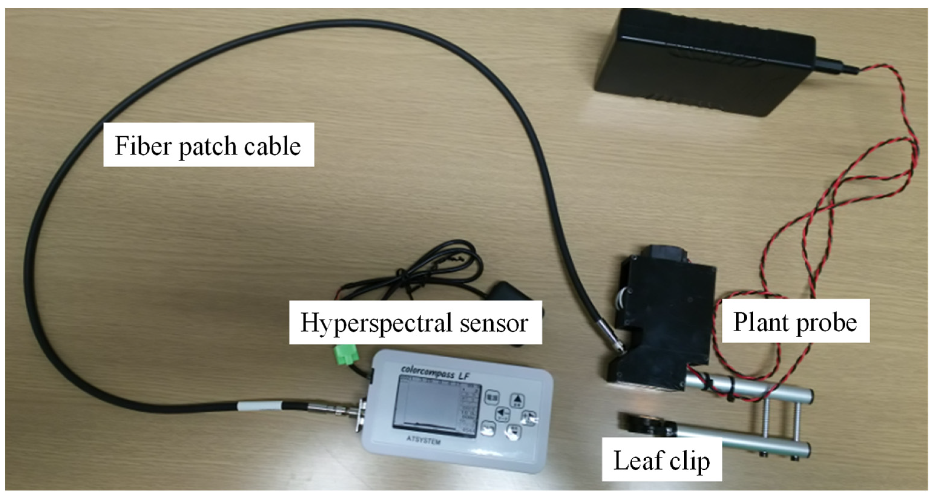
We used a spectrometer with a complementary metal-oxide semiconductor (CMOS) sensor (C12880MA-10, Hamamatsu Photonics) and a shape-memory alloy (SMA)–SMA fiber patch cable (M25L05, Thorlabs, Newton, NJ, USA) with a 0.22 numerical aperture to measure reflectance with a leaf clip (Figure 3, colorcompass-LF). The grating equations provided by Hamamatsu Photonics were applied and then the spectral resolution was resampled in 5 nm bands across the entire wavelength domain from 400 to 850 nm. The plant probe has a halogen light source, and its leaf clip has replaceable white and black background standards.
The reflectance of the target was calculated using the following equation:
ρ λ = S λ D λ W λ D λ
where S, W, and D represent the target, a diffuse reflectance standard, and dark current, respectively, at wavelength λ (in nm). We applied five different preprocessing techniques to remove the baseline influence and to compensate for additive or multiplicative effects in the spectral data. All calculations were conducted using R statistical software, version 4.0.2 [31].
We collected leaf samples via punching and used them for pigment concentration measurements in N, N-dimethylformamide extract with a dual-beam scanning ultraviolet-visible spectrophotometer (UV-1280, Shimadzu, Kyoto, Japan). We used the following equations to quantify chlorophyll content [32]:
C a + b = C a + C b
C a = 12 A 663.8 3.11 A 646.8
C b = 20.78 A 646.8 4.88 A 663.8
where C a + b , C a , and C b represent the pigment contents of total chlorophyll and chlorophyll a and b, where A is absorbance and the subscripts are the wavelengths in nm.

2.2. Preprocessing of Raw Reflectance Data

Before we used the reflectance measurements from the colorcompass-LF to estimate chlorophyll content, we investigated some denoising techniques. These techniques are used to reduce noninformative signal and improve the signal-to-noise ratio (SNR) of the spectra and include scatter-correction methods, such as detrending (DT), multiple scattering correction (MSC), standard normal transformation (SNV), and derivative algorithms [33]. Derivative algorithms, such as the first derivative of reflectance (FDR) and continuum removal (CR), have been used to assess vegetation properties, such as leaf area index, accumulation of leaf nitrogen, and chlorophyll content based on hyperspectral reflectance data [34,35]. We tested these five preprocessing methods as well as the original reflectance (OR).

2.2.1. First-Derivative Reflectance (FDR)

This is an effective technique for removing background effects and enhancing both subtle and weak spectral features that are useful for evaluating target parameters [36]. It has been used to enhance specific points, such as the green peak and the red-edge inflection point (REIP) [37].

2.2.2. Continuum Removal (CR)

This technique, proposed by Clark [38], entails removing the continuous features of the spectra and is often used to isolate specific absorption features present in a spectrum to partially minimize the noise. The continuum is represented by a mathematical function used to separate and highlight the specific absorption bands of the reflectance spectrum [39]. This method enables the normalization of a spectrum and thereby facilitates the identification of informative absorption features across the visible–NIR spectrum.

2.2.3. Detrending (DT)

This is a simple baseline correction method in which the baseline is assumed to be a second-degree polynomial function of wavelength and is subtracted from the spectrum. This technique has also been used to account for variation in baseline shift and curvilinearity [40].

2.2.4. Standard Normal Variate (SNV)

The SNV correction can correct multiple types of scattering noise (such as the influence of sample size and scattering interference) caused by the surface structure of a sample. This scatter correction is a manual row-oriented transformation that standardizes a spectrum using its mean and standard deviation. The process is initiated by calculating the mean and standard deviation for each spectrum i of m × 1 column vector xi, after which every data point of xij is subtracted from the mean and the result is divided by the standard deviation. This is mathematically expressed as follows:
x ij ( SNV ) = ( x ij x ¯ x ) / s ( x i )
However, since there is no fitting of least squares in the parameter estimation of SNV, this method is very sensitive to any noisy points in a spectrum. This pretreatment method may therefore have negative effects in cases where numerous noisy points occur in a spectrum [40].

2.2.5. Multiplicative Scatter Correction (MSC)

According to Shao et al. [41] and Liu et al. [42], MSC has similar benefits to SNV and can be used to effectively remove the baseline effect (both translation and offset) in spectra [43]. This correction is performed by applying multiplicative and additive spectral corrections to the original spectra corresponding to the mean. The resulting corrected spectra have a relatively consistent baseline. For each j of m wavelengths, the mean of all n spectra is calculated and referred to as the m × 1 column vector of a standard spectrum m. A simple linear regression (xij = αi + βimj + eij) is then performed on each i spectrum of m × 1 column vector xi of n spectra in X (as the dependent variable) relative to the m × 1 vector m (as the independent variable). The solution is calculated using the ordinary least squares (LS) method, and the regression coefficient parameter βi and intercept αi are used to correct the baseline scatter by subtracting αi from each spectrum xi and dividing by β1 as follows:
xij(MSC) = (xij − αi)/βi

2.3. Variable Selection Methods Applied in This Study

We used three groups of variable selection methods based on partial least squares (PLS)—filter, wrapper, and embedded methods (Table 1)—on the spectral data [44,45]. The filter methods we used were loading weights (LW), regression coefficients (RC), and variable importance in projection (VIP); the wrapper methods were backward variable elimination (BVE), competitive adaptive reweighted sampling (CARS), genetic algorithm (GA), iterative predictive weighting (IPW), PLS with Martens’ uncertainty test (MUT), the regularized elimination procedure (REP), sub-window permutation analysis (SwPA), and uninformative variable elimination (UVE); and the embedded methods we used were backward- and forward-interval PLS (BiPLS and FiPLS) and sparse PLS (SPLS).
When using the filter methods, the high- and low-sensitivity variables are selected according to (a) the maximum absolute loading weights calculated from the principal factors (LW method) [46]; (b) the accumulated loading weights of each component (VIP method) [47]; or (c) their regression coefficients (RC method) [45].
With respect to the wrapper methods, BVE is a backward-iterative step-by-step PLS-oriented method for selecting spectral variables, and its objective is to build a correct model with as few variables as possible [44]. Monte Carlo sampling with a PLS regression coefficient is applied in the CARS method, and variables with larger regression-coefficient weights are used as a new subset to establish a PLS model [48]. The GA method is an adaptive heuristic search algorithm centered on the evolutionary concepts of natural selection and genetics, while the IPW method involves the cyclic repetition of PLS regression. This calculates predictor importance based on the absolute value of the regression coefficient and then computes the standard deviation of the predictor; the predictors are then multiplied by their importance in the next cycle [49]. In the MUT method, the principle of jackknifing is used to estimate the standard errors of the regression coefficients, which are then divided by these standard errors to yield t-test statistics [50]. The REP method involves a stepwise elimination and a stability-based variable selection procedure in which the samples are randomly split into a predefined number of training and test data sets [45]. In the SwPA method, the influence of each variable is evaluated without considering the influence of the other variables [51]. In the UVE method, artificial noise variables are added to the data and all original variables that are less informative before the addition of artificial noise are removed [52].
In the embedded methods, variable selection is conducted at the component level. In the iPLS methods, the data are divided into nonoverlapping intervals and a separate PLS model is built for each interval to identify the most useful variable [53]. In FiPLS, the subinterval with the smallest cross-validated prediction error is selected, while in BiPLS the subintervals with the largest error are removed [45]. The SPLS method combines variable selection and modeling in a single-step procedure [54]. The details of each method are summarized by Mehmood et al. [45].

2.4. Regression Models Based on Machine Learning Algorithms

The measurements were divided into three groups (a training dataset [50%], a validation dataset [25%], and a test data dataset [25%]) using a stratified sampling approach. To apply this strategy, all measurements were divided into five groups based on slag treatments and 50% of the groups were selected as training data, which were used for generating regression models according to a random number assigned to each group. Next, 50% of the remaining measurements were selected as validation data, which were used to optimize the hyperparameters of the machine learning algorithms. Finally, the last group was used as test data to evaluate model accuracy. This procedure was repeated 100 times to increase the robustness of the results before the regression models were generated. After running the preprocessing and variable selection procedures, we generated regression models based on Cubist, which is a tool that has been shown globally to perform best in studies related to machine learning algorithms [55,56]. Cubist is a rule-based model tree approach, and its leaves are expressed as multivariate linear regression models. The number of committee models (committee) and neighbors (neighbor) used for correcting the model predictions were optimized using the “Cubist” package [57]. Adjusting the committee models has a similar boosting effect. A nearest-neighbor algorithm was applied to the leaf nodes to implement an ensemble approach combination.

2.5. Performance Assessment

To assess the performance of the regression models, we calculated the ratio of performance to deviation (RPD, Equation (7)) [58] and the root mean square error (RMSE, Equation (8)). Each method was classified into three categories based on its RPD: ‘A’ (RPD > 2.0), ‘B’ (1.4 ≤ RPD ≤ 2.0), or ‘C’ (RPD < 1.4). Models classified as ‘A’ or ‘B’ were assumed to have the potential to estimate chlorophyll content [59].
RPD = SD / RMSE ,
RMSE = 1 n i = 0 n y i ^ y i 2 ,
where SD is the standard deviation of the chlorophyll content in the test data, n is the number of samples, y i is the measured chlorophyll content, and y i ^ is the estimated chlorophyll content.
The R packages used to apply the various preprocessing and variable selection methods are listed in Table 2.
The variance principle has been used in evaluating the sensitivity of spectral wavelengths [52]. For wavelength i (in nm), the sensitivity Si is calculated as follows:
S i = Var ( f X 400 , , X i , , X 850 f X ¯ Var Y ,  
where Var is the variation, f () is the prediction of spectra due to the variation in wavelength i with other wavelengths held constant at their mean values, f ( X ¯ ) is the estimated value based on the mean reflectance, and Y represents the measured chlorophyll content. Once we had calculated Si, we converted the scores to percentages.

3. Results

3.1. Chlorophyll Content for Each Cultivar

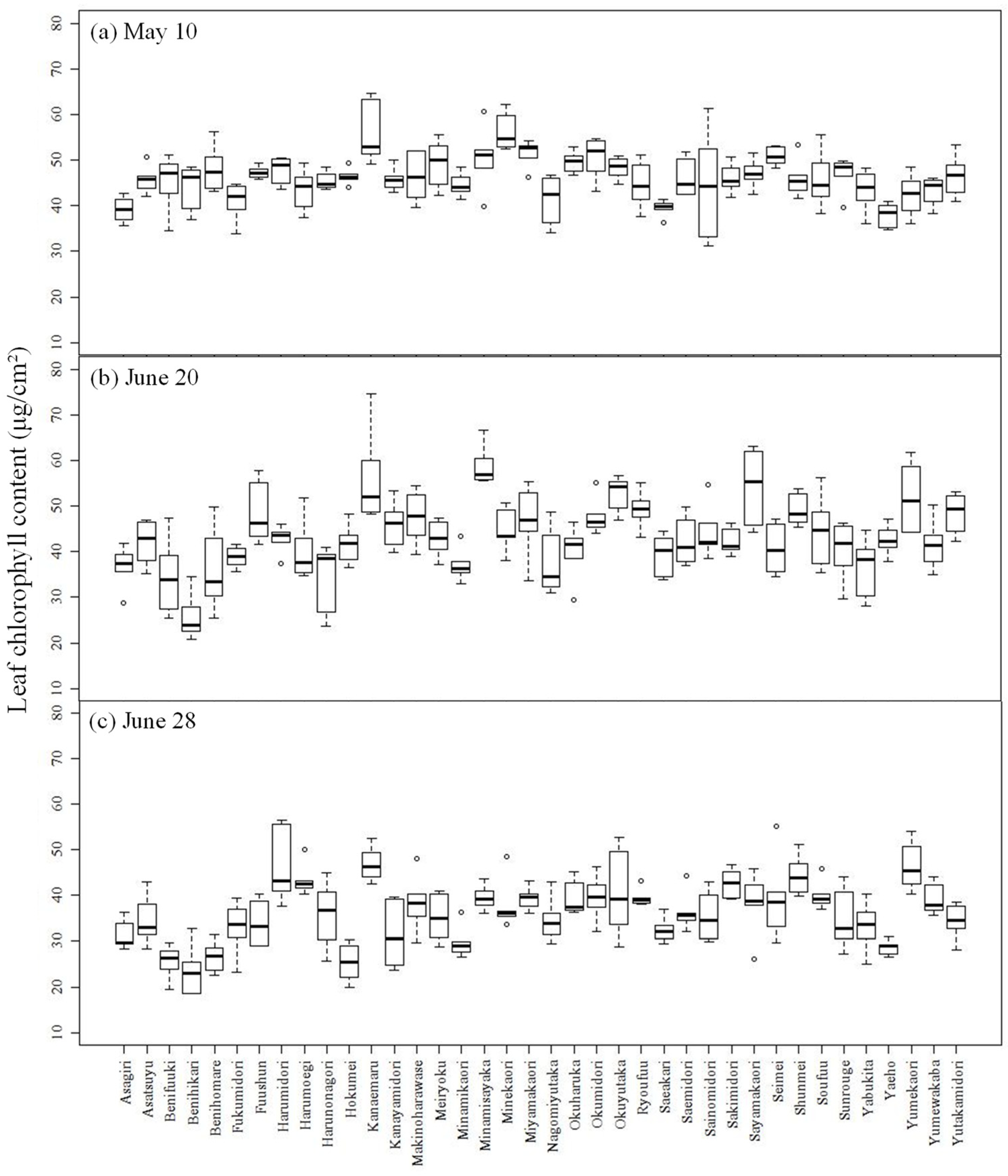
The chlorophyll content per cm2 of leaf area was 31.26–64.56 μg, 20.71–74.65 μg, and 18.59–56.52 μg on 10 May, 20 June, and 28 June, respectively (Figure 4). The chlorophyll content of the third leaves therefore decreased over time, although these changes were relatively small for the Harumidori, Harumoegi, and Shunmei cultivars. Asagiri (mean: 39.19 μg), Saeakari (39.55 μg), and Yaeho (37.98 μg) had the lowest chlorophyll content. Although the black tea cultivars (Benifuuki, Benihikari, and Benihomare) had a moderate chlorophyll content on 10 May, it was low in June, with mean values of 25.58–35.87 μg and 23.09–26.86 μg on 20 and 28 June, respectively (Figure 3).

3.2. Spectral Reflectance According to Preprocessing Treatment

For OR, the negative correlation of spectral reflectance with chlorophyll content was confirmed near the green peak (525–630 nm) and the red edge inflection point (REIP, 710 nm) for all sampling dates. The lowest correlation coefficients were −0.60, −0.71, and −0.67 for the three measurement dates, respectively (Figure 5). After preprocessing, the correlations with chlorophyll content became stronger over these two domains and were even positive for 10 May when FDR preprocessing was used. We observed similar patterns for the other dates, although the negative correlation over the green peak became weaker than for the OR. When DT was used, the correlation between spectral reflectance and chlorophyll content at 610–620 nm was positive and significant (r = 0.67, 0.76, and 0.70 for 10 May, 20 June, and 28 June, respectively; p < 0.001). There were almost no differences in between the results yielded by MSC and SNV preprocessing, with which high correlations were observed at 400–500 nm (r = 0.76, 0.82, and 0.84 at 485 nm for the three dates, respectively; Figure 4).

3.3. Wavelengths Selected by the Variable Selection Methods

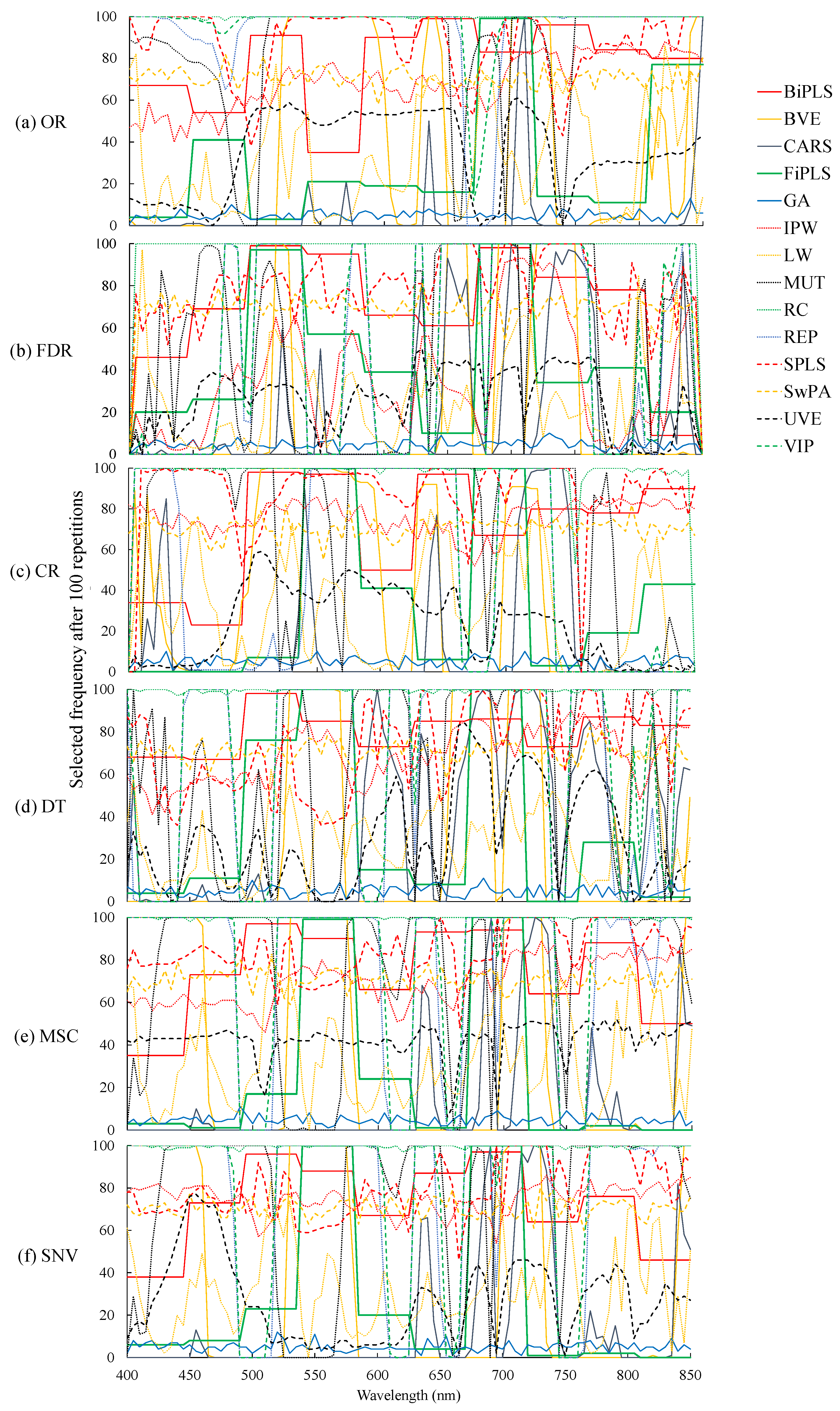
In general, of the 14 variable selection methods, GA selected the smallest number of bands, with an average of <5 selected in 100 repetitions for all preprocessing methods (4.5, 4.1, 4.5, 4.4, 4.2, and 4.5 for OR, FDR, CR, DT, MSC, and SNV, respectively; Figure 6). In contrast, RC selected > 88 bands, with the highest number (91) selected when using OR. The frequencies selected for the red-edge domain were high, and wavelengths of 685–730 nm were selected more than 30 times for all preprocessing techniques and variable selection methods except for GA. The reflectance over the green peak (around 550 nm) was also selected more than 30 times for FDR and DT, again except when GA was used (Figure 5).

3.4. Accuracy Assessment

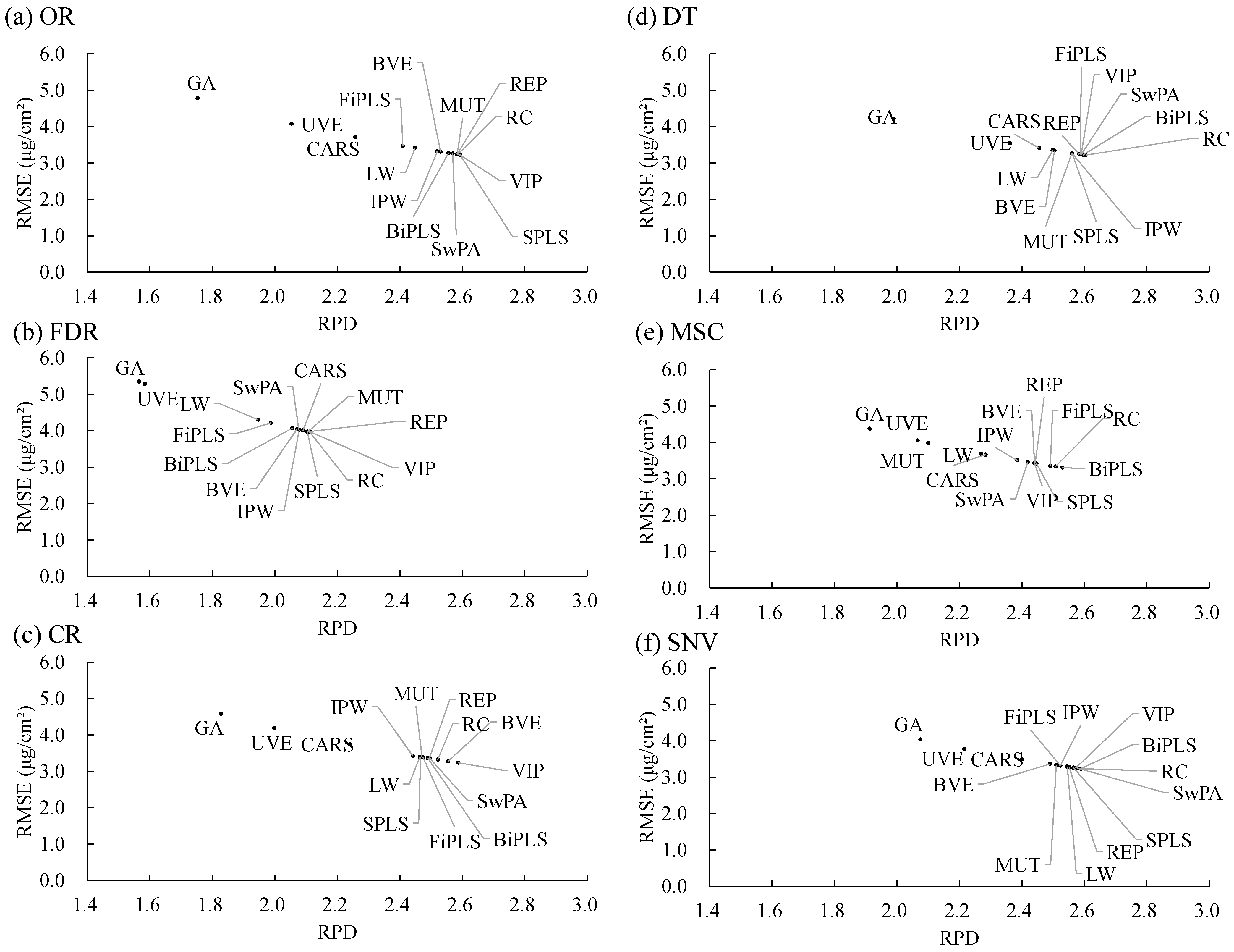
All RPD values were >1.4, so all combinations of preprocessing and variable selection methods were acceptable for estimating chlorophyll content in tea leaves (Table 3). In fact, the minimum RPD value, for the combination of FDR with GA, was 1.57. However, the FDR, CR, and MSC preprocessing techniques did not improve chlorophyll-estimation accuracy and indeed resulted in a lower accuracy than OR.
The most effective preprocessing technique was DT, whose RPD values were 1.99–2.60 (mean: 2.49). The most effective variable selection method was RC, which had RPD values of 2.11–2.60 (mean: 2.50). These methods thus both fell into category A. The best combination of preprocessing technique and variable selection method was therefore DT–RC, which achieved an RPD of 2.60 and an RMSE of 3.21 μg cm−2 (Table 3 and Table 4; Figure 7).

3.5. Sensitivity Analysis

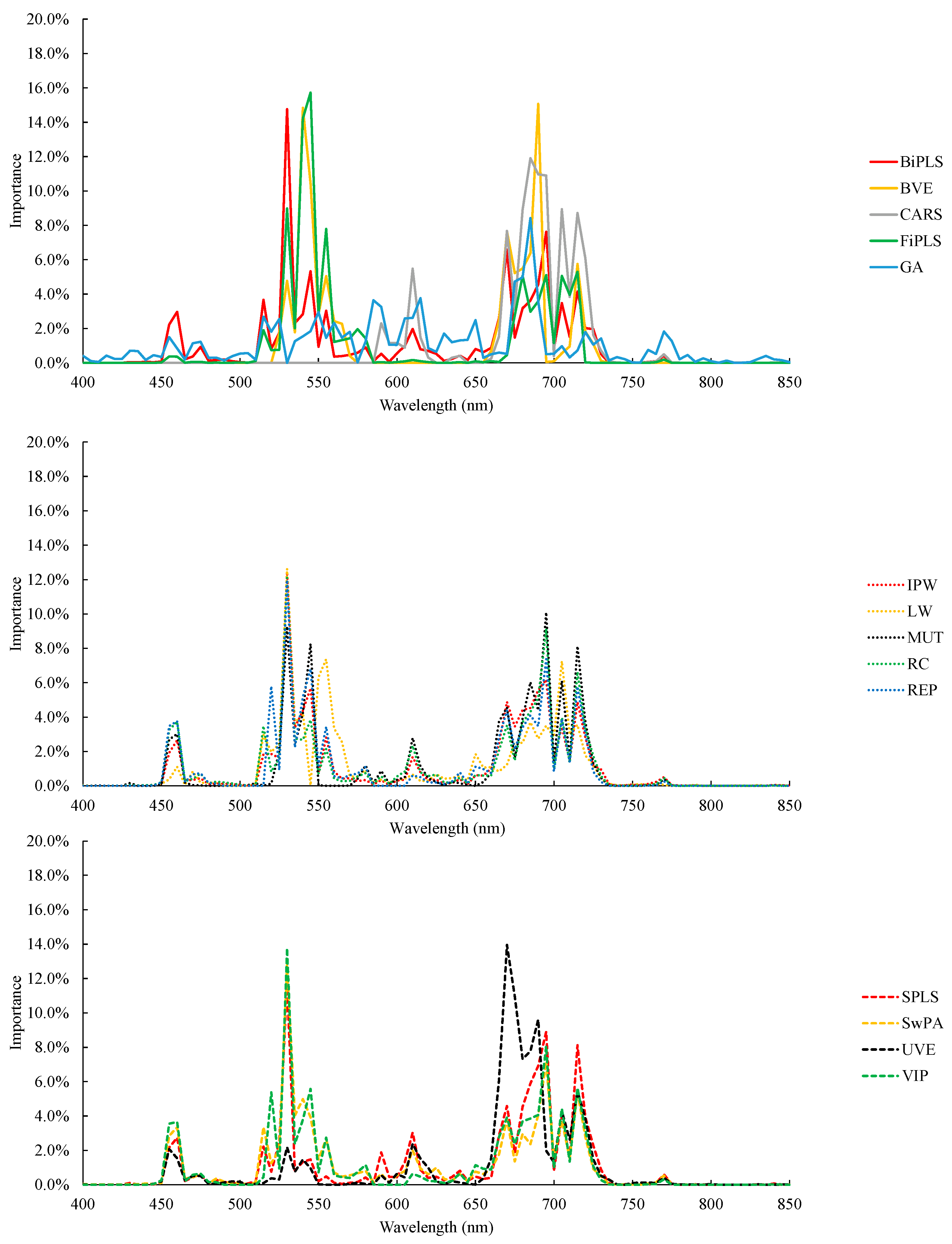
We conducted a sensitivity analysis on the regression models produced using DT with each of the 14 variable selection methods (Figure 8). Most of the methods identified the green peak and REIP as important, although the importance of the green peak was lower when using the CARS and UVE methods, which emphasized the importance of the REIP. In addition, the most important wavelength in the green peak differed slightly among the selection methods—it was 530 nm when using BiPLS, CARS, LW, MUT, RC, REP, SPLS, SwPA, and VIP but 550 nm for BVE, FiPLS, and IPW (Figure 7).

4. Discussion

4.1. Relationship between Reflectance Recorded Using the Compact Spectrometer and Chlorophyll Content

Chlorophyll content increases with increasing nitrogen, which leads to lower reflectance due to the strong absorption of chlorophyll a and b under blue (410–470 nm) and red (644.8–670 nm) light, respectively [65,66]. Low reflectance in these regions was observed using the colorcompass-LF. In previous studies, reflectance at 550 nm, which is frequently reported as the green peak, has been used to estimate chlorophyll content [67,68], and there is a marked reduction in reflectance at the green peak when chlorophyll content is high. However, some studies have reported that chlorophyll contributes to reflectance at 550 nm, especially when there is a low anthocyanin content against a background of high chlorophyll content [69]. The red edge has also been used to estimate chlorophyll content, and in this case shifts to longer wavelengths to indicate a higher chlorophyll content [70,71].
When a C12880MA-10 hyperspectral sensor was used to measure the reflectance of Zizania latifolia with the sun as the light source and without a plant probe, there was a decrease in reflectance at 800 nm as a result of changes in sun altitude [56]. This may contribute to uncertainty in reflectance data acquired using this sensor. Additionally, the relative sensitivity of this sensor is less than 0.5 at 700 nm, so reflectance measured at the REIP is not suitable for chlorophyll-content estimation [72]. In the present study, this problem was resolved by using a plant probe. This facilitated accurate reflectance measurements without negative effects caused by changes in sun altitude or objects behind the leaf such as the observer’s hand, tea petioles, or other leaves [73,74]. Under these conditions, reflectance near the REIP can be used to estimate chlorophyll content, as our results confirm.
In earlier studies, the reflectance data from an ASD FieldSpec4 unit (Analytical Spectral Devices, Boulder, CO, USA) were used for estimating chlorophyll content of tea leaves and the root-mean-square errors from 3.04 to 8.94 μg cm−2 were confirmed [75,76]. Although the leaf samples were not same, our reflectance measurement system (colorcompass-LF) estimated the chlorophyll content with almost the same accuracy as the high-specification spectrometer (ASD FieldSpec4).

4.2. Comparison of Variable Selection Methods and Preprocessing Techniques

Detrending was selected as the best preprocessing technique for all 38 cultivars, and the combination of RC and DT was the best when the results were merged after all 100 repetitions (Table 5). However, when considering the repetitions individually, this combination was selected as the best only eight times out of 100. The BiPLS variable selection method was selected as the best 16 times (seven, four, and three times with DT, MSC, and SNV, respectively, and once each with OR and CR), while RC was selected 15 times in total. Generally, the selection methods that assigned a relatively high importance to the green peak were effective (BiPLS, FiPLS, and RC were selected as the best selection methods 16, 8, and 15 times, respectively) while those that assigned <3.0% importance to the green peak (GARS and GA) were never selected.
All selection methods assigned a high importance to the REIP, which is usually necessary for the accurate estimation of chlorophyll content [77,78]. However, relative sensitivity was <0.5 at 700 nm [72], so results from a compact spectrometer using this domain alone would be insufficient for estimating chlorophyll content.
Ram et al. [79] reported that anthocyanin induction is strongly influenced by low nitrogen concentration. Anthocyanin reflectance differs between the green peak and the red edge: wavelengths at the red edge are absorbed by chlorophyll but not by anthocyanin, whereas light absorption by anthocyanin is highest at the green peak [80]. Cultivars producing high-quality black tea usually have higher levels of catechins and higher ratios of catechins to amino acids than those producing high-quality green tea [81]. Anthocyanin-rich tea cultivars, such as Sunrouge, were also included in this study, and measurements for Sunrouge provided RPD values of >2.4 for RC and VIP but of 1.63 for GA. Differences between results produced using different variable selection methods were particularly marked for Asagiri: the RPD value for RC was 3.23 and that for GA was 1.70. In contrast, the RPD values were consistently >2.0 for Benihikari, Benihomare, Fuushun, Hokumei, Kanayamidori, Okuyutaka, Sayamakaori, and Yutakamidori, regardless of the variable selection method used. Therefore, combining the green peak and REIP was effective for taking the effects of anthocyanin on reflectance into account.

5. Conclusions

In this study, we acquired hyperspectral data using a novel system (the colorcompass-LF) comprising a complementary metal-oxide semiconductor (CMOS) sensor (C12880MA-10, Hamamatsu Photonics), a shape-memory alloy (SMA)–SMA fiber patch cable (M25L05, Thorlabs), and a plant probe with a leaf clip. To evaluate the performance of this system, we estimated the chlorophyll content of tea leaves using the reflectance measured by this device. We also compared a range of combinations of variable selection method and preprocessing technique for analyzing these data. All combinations were acceptable for evaluating the chlorophyll content of the 38 tea cultivars sampled based on the data collected. The best combination was RC-DT, with an RPD of 2.60 and an RMSE of 3.21 μg cm−2. The high importance of reflectance in the red edge region indicated that accuracy was high even though the relative sensitivity of the C12880MA-10 was <0.5 around this region. These results confirm that using a plant probe effectively counteracts the limitations of the components of this system when used in isolation.
The proposed method is affordable, making it practical for consumers to use. This system would also facilitate affordable field-scale monitoring using drones and whisk broom scanning.

Author Contributions

R.S. and Y.H. conceived and designed the experiments. R.S. analyzed the data and wrote the manuscript. R.S. and Y.H. conducted the measurements. All authors have read and agreed to the published version of the manuscript.

Funding

This research was supported by the Agriculture, Forestry, and Fisheries Research Council [19191026].

Data Availability Statement

The data presented in this study are made available by contacting the corresponding author.

Acknowledgments

We thank members of the Laboratory of Macroecology, Shizuoka University, for assisting with field work.

Conflicts of Interest

The authors have no conflict of interest to declare.

References

  1. Katoh, M.; Katoh, Y.; Kinoshita, T.; Yamaguchi, Y.; Omori, M. Identification of Tea Cultivar by Amolified DNA Fragment Length Polymorphism (AFLP) Using Black Teas as Sample. J. Jpn. Soc. Food Sci. Technol. Nippon Shokuhin Kagaku Kogaku Kaishi 2010, 57, 389–394. [Google Scholar] [CrossRef] [Green Version]
  2. Hazra, A.; Dasgupta, N.; Sengupta, C.; Bera, B.; Das, S. Tea: A Worthwhile, Popular Beverage Crop Since Time Immemorial. Agron. Crops 2019, 1, 507–531. [Google Scholar] [CrossRef]
  3. Korus, A. Effect of preliminary and technological treatments on the content of chlorophylls and carotenoids in kale (Brassica oleracea L. var. Acephala). J. Food Process. Preserv. 2013, 37, 335–344. [Google Scholar] [CrossRef]
  4. Zhang, H.; Duan, Z.; Li, Y.Y.; Zhao, G.Y.; Zhu, S.M.; Fu, W.; Peng, T.; Zhao, Q.Z.; Svanberg, S.; Hu, J.D. Vis/NIR reflectance spectroscopy for hybrid rice variety identification and chlorophyll content evaluation for different nitrogen fertilizer levels. R. Soc. Open Sci. 2019, 6, 191132. [Google Scholar] [CrossRef] [Green Version]
  5. Colla, G.; Cardarelli, M.; Fiorillo, A.; Rouphael, Y.; Rea, E. Enhancing Nitrogen Use Efficiency in Cucurbitaceae Crops by Grafting. In Proceedings of the International Symposium on Advanced Technologies and Management Towards Sustainable Greenhouse Ecosystems: Greensys2011, Athens, Greece, 5–10 June 2011; Volume 952, pp. 863–869. [Google Scholar]
  6. Wang, L.F.; Park, S.C.; Chung, J.O.; Baik, L.H.; Park, S.K. The compounds contributing to the greenness of green tea. J. Food Sci. 2004, 69, S301–S305. [Google Scholar] [CrossRef]
  7. Wang, K.B.; Liu, F.; Liu, Z.H.; Huang, J.A.; Xu, Z.X.; Li, Y.H.; Chen, J.H.; Gong, Y.S.; Yang, X.H. Analysis of chemical components in oolong tea in relation to perceived quality. Int. J. Food Sci. Technol. 2010, 45, 913–920. [Google Scholar] [CrossRef]
  8. Prado-Cabrero, A.; Beatty, S.; Howard, A.; Stack, J.; Bettin, P.; Nolan, J.M. Assessment of lutein, zeaxanthin and meso-zeaxanthin concentrations in dietary supplements by chiral high-performance liquid chromatography. Eur. Food Res. Technol. 2016, 242, 599–608. [Google Scholar] [CrossRef] [Green Version]
  9. Das, A.; Guyer, L.; Hortensteiner, S. Chlorophyll and Chlorophyll Catabolite Analysis by HPLC. Plant Senescence Methods Protoc. 2018, 1744, 223–235. [Google Scholar] [CrossRef] [Green Version]
  10. Leon, A.P.; Vina, S.Z.; Frezza, D.; Chaves, A.; Chiesa, A. Estimation of chlorophyll contents by correlations between SPAD-502 meter and chroma meter in butterhead lettuce. Commun. Soil Sci. Plant Anal. 2007, 38, 2877–2885. [Google Scholar] [CrossRef]
  11. Peng, S.B.; Garcia, F.V.; Laza, R.C.; Cassman, K.G. Adjustment for Specific Leaf Weight Improves Chlorophyll Meter’s Estimate of Rice Leaf Nitrogen Concentration. Agron. J. 1993, 85, 987–990. [Google Scholar] [CrossRef]
  12. Sano, T.; Horie, H.; Matsunaga, A.; Hirono, Y. Effect of shading intensity on morphological and color traits and on chemical components of new tea (Camellia sinensis L.) shoots under direct covering cultivation. J. Sci. Food Agric. 2018, 98, 5666–5676. [Google Scholar] [CrossRef] [PubMed]
  13. Feret, J.B.; Gitelson, A.A.; Noble, S.D.; Jacquemoud, S. PROSPECT-D: Towards modeling leaf optical properties through a complete lifecycle. Remote Sens. Environ. 2017, 193, 204–215. [Google Scholar] [CrossRef] [Green Version]
  14. Piegari, E.; Gossn, J.I.; Grings, F.; Bernadas, V.B.; Juarez, A.B.; Mateos-Naranjo, E.; Trilla, G.G. Estimation of leaf area index and leaf chlorophyll content in Sporobolus densiflorus using hyperspectral measurements and PROSAIL model simulations. Int. J. Remote Sens. 2021, 42, 1181–1200. [Google Scholar] [CrossRef]
  15. Dao, P.D.; He, Y.H.; Proctor, C. Plant drought impact detection using ultra-high spatial resolution hyperspectral images and machine learning. Int. J. Appl. Earth Obs. Geoinf. 2021, 102, 102364. [Google Scholar] [CrossRef]
  16. Doktor, D.; Lausch, A.; Spengler, D.; Thurner, M. Extraction of Plant Physiological Status from Hyperspectral Signatures Using Machine Learning Methods. Remote Sens. 2014, 6, 12247–12274. [Google Scholar] [CrossRef] [Green Version]
  17. Zhang, C.; Zhao, Y.Y.; Yan, T.Y.; Bai, X.L.; Xiao, Q.L.; Gao, P.; Li, M.; Huang, W.; Bao, Y.D.; He, Y.; et al. Application of near-infrared hyperspectral imaging for variety identification of coated maize kernels with deep learning. Infrared Phys. Technol. 2020, 111, 103550. [Google Scholar] [CrossRef]
  18. Gautam, D.; Lucieer, A.; Watson, C.; McCoull, C. Lever-arm and boresight correction, and field of view determination of a spectroradiometer mounted on an unmanned aircraft system. ISPRS J. Photogramm. Remote Sens. 2019, 155, 25–36. [Google Scholar] [CrossRef]
  19. Zarco-Tejada, P.J.; Berjon, A.; Lopez-Lozano, R.; Miller, J.R.; Martin, P.; Cachorro, V.; Gonzalez, M.R.; de Frutos, A. Assessing vineyard condition with hyperspectral indices: Leaf and canopy reflectance simulation in a row-structured discontinuous canopy. Remote Sens. Environ. 2005, 99, 271–287. [Google Scholar] [CrossRef]
  20. Feret, J.B.; Francois, C.; Asner, G.P.; Gitelson, A.A.; Martin, R.E.; Bidel, L.P.R.; Ustin, S.L.; le Maire, G.; Jacquemoud, S. PROSPECT-4 and 5: Advances in the leaf optical properties model separating photosynthetic pigments. Remote Sens. Environ. 2008, 112, 3030–3043. [Google Scholar] [CrossRef]
  21. Sonobe, R.; Yamashita, H.; Mihara, H.; Morita, A.; Ikka, T. Hyperspectral reflectance sensing for quantifying leaf chlorophyll content in wasabi leaves using spectral pre-processing techniques and machine learning algorithms. Int. J. Remote Sens. 2021, 42, 1311–1329. [Google Scholar] [CrossRef]
  22. Sonobe, R.; Wang, Q. Nondestructive assessments of carotenoids content of broadleaved plant species using hyperspectral indices. Comput. Electron. Agric. 2018, 145, 18–26. [Google Scholar] [CrossRef]
  23. Sonobe, R.; Miura, Y.; Sano, T.; Horie, H. Monitoring Photosynthetic Pigments of Shade-Grown Tea from Hyperspectral Reflectance. Can. J. Remote Sens. 2018, 44, 104–112. [Google Scholar] [CrossRef]
  24. Sonobe, R.; Yamashita, H.; Mihara, H.; Morita, A.; Ikka, T. Estimation of Leaf Chlorophyll a, b and Carotenoid Contents and Their Ratios Using Hyperspectral Reflectance. Remote Sens. 2020, 12, 3265. [Google Scholar] [CrossRef]
  25. Sonobe, R.; Miura, Y.; Sano, T.; Horie, H. Estimating leaf carotenoid contents of shade-grown tea using hyperspectral indices and PROSPECT-D inversion. Int. J. Remote Sens. 2018, 39, 1306–1320. [Google Scholar] [CrossRef]
  26. Sonobe, R.; Hirono, Y.; Oi, A. Quantifying chlorophyll-aandbcontent in tea leaves using hyperspectral reflectance and deep learning. Remote Sens. Lett. 2020, 11, 933–942. [Google Scholar] [CrossRef]
  27. Uto, K.; Seki, H.; Saito, G.; Kosugi, Y.; Komatsu, T. Development of a Low-Cost Hyperspectral Whiskbroom Imager Using an Optical Fiber Bundle, a Swing Mirror, and Compact Spectrometers. IEEE J. Sel. Top. Appl. Earth Obs. Remote Sens. 2016, 9, 3909–3925. [Google Scholar] [CrossRef]
  28. Hovi, A.; Forsstrom, P.; Mottus, M.; Rautiainen, M. Evaluation of Accuracy and Practical Applicability of Methods for Measuring Leaf Reflectance and Transmittance Spectra. Remote Sens. 2018, 10, 25. [Google Scholar] [CrossRef] [Green Version]
  29. Balabin, R.M.; Smirnov, S.V. Variable selection in near-infrared spectroscopy: Benchmarking of feature selection methods on biodiesel data. Anal. Chim. Acta 2011, 692, 63–72. [Google Scholar] [CrossRef]
  30. Sonobe, R.; Sugimoto, Y.; Kondo, R.; Seki, H.; Sugiyama, E.; Kiriiwa, Y.; Suzuki, K. Hyperspectral wavelength selection for estimating chlorophyll content of muskmelon leaves. Eur. J. Remote Sens. 2021, 54, 512–523. [Google Scholar] [CrossRef]
  31. R Core Team. R: A Language and Environment for Statistical Computing. Available online: https://www.R-project.org/ (accessed on 24 October 2022).
  32. Wellburn, A.R. The spectral determination of chlorophyll a and chlorophyll b, as well as total carotenoids, using various solvents with spectrophotometers of different resolution. J. Plant Physiol. 1994, 144, 307–313. [Google Scholar] [CrossRef]
  33. Rinnan, A.; van den Berg, F.; Engelsen, S.B. Review of the most common pre-processing techniques for near-infrared spectra. Trac-Trends Anal. Chem. 2009, 28, 1201–1222. [Google Scholar] [CrossRef]
  34. Ali, A.; Imran, M.M. Evaluating the potential of red edge position (REP) of hyperspectral remote sensing data for real time estimation of LAI & chlorophyll content of kinnow mandarin (Citrus reticulata) fruit orchards. Sci. Hortic. 2020, 267, 11. [Google Scholar] [CrossRef]
  35. Boloorani, A.D.; Ranjbareslamloo, S.; Mirzaie, S.; Bahrami, H.A.; Mirzapour, F.; Tehrani, N.A. Spectral behavior of Persian oak under compound stress of water deficit and dust storm. Int. J. Appl. Earth Obs. Geoinf. 2020, 88, 16. [Google Scholar] [CrossRef]
  36. Meng, X.T.; Bao, Y.L.; Liu, J.G.; Liu, H.J.; Zhang, X.L.; Zhang, Y.; Wang, P.; Tang, H.T.; Kong, F.C. Regional soil organic carbon prediction model based on a discrete wavelet analysis of hyperspectral satellite data. Int. J. Appl. Earth Obs. Geoinf. 2020, 89, 102111. [Google Scholar] [CrossRef]
  37. Cho, M.A.; Skidmore, A.K. A new technique for extracting the red edge position from hyperspectral data: The linear extrapolation method. Remote Sens. Environ. 2006, 101, 181–193. [Google Scholar] [CrossRef]
  38. Clark, R.N.; Roush, T.L. Reflectance spectroscopy: Quantitative analysis techniques for remote sensing applications. J. Geophys. Res. 1984, 89, 6329–6340. [Google Scholar] [CrossRef]
  39. Mutanga, O.; Skidmore, A.K. Narrow band vegetation indices overcome the saturation problem in biomass estimation. Int. J. Remote Sens. 2004, 25, 3999–4014. [Google Scholar] [CrossRef]
  40. Barnes, R.J.; Dhanoa, M.S.; Lister, S.J. Standard Normal Variate Transformation and De-Trending of Near-Infrared Diffuse Reflectance Spectra. Appl. Spectrosc. 1989, 43, 772–777. [Google Scholar] [CrossRef]
  41. Shao, Y.N.; He, Y.; Bao, Y.D.; Mao, J.Y. Near-Infrared Spectroscopy for Classification of Oranges and Prediction of the Sugar Content. Int. J. Food Prop. 2009, 12, 644–658. [Google Scholar] [CrossRef]
  42. Liu, Y.D.; Sun, X.D.; Ouyang, A.G. Nondestructive measurement of soluble solid content of navel orange fruit by visible-NIR spectrometric technique with PLSR and PCA-BPNN. LWT Food Sci. Technol. 2010, 43, 602–607. [Google Scholar] [CrossRef]
  43. Geladi, P.; MacDougall, D.; Martens, H. Linearization and scatter-correction for near infrared reflectance spectra of meat. Appl. Spectrosc. 1985, 39, 491–500. [Google Scholar] [CrossRef]
  44. Pierna, J.A.F.; Abbas, O.; Baeten, V.; Dardenne, P. A Backward Variable Selection method for PLS regression (BVSPLS). Anal. Chim. Acta 2009, 642, 89–93. [Google Scholar] [CrossRef] [PubMed]
  45. Mehmood, T.; Liland, K.H.; Snipen, L.; Saebo, S. A review of variable selection methods in Partial Least Squares Regression. Chemom. Intell. Lab. Syst. 2012, 118, 62–69. [Google Scholar] [CrossRef]
  46. Wang, Y.G.; Gao, Y.; Yu, X.Z.; Wang, Y.Y.; Deng, S.; Gao, J.M. Rapid Determination of Lycium barbarum Polysaccharide with Effective Wavelength Selection Using Near-Infrared Diffuse Reflectance Spectroscopy. Food Anal. Methods 2016, 9, 131–138. [Google Scholar] [CrossRef]
  47. Chong, I.G.; Jun, C.H. Performance of some variable selection methods when multicollinearity is present. Chemom. Intell. Lab. Syst. 2005, 78, 103–112. [Google Scholar] [CrossRef]
  48. Fan, S.X.; Zhang, B.H.; Li, J.B.; Huang, W.Q.; Wang, C.P. Effect of spectrum measurement position variation on the robustness of NIR spectroscopy models for soluble solids content of apple. Biosyst. Eng. 2016, 143, 9–19. [Google Scholar] [CrossRef]
  49. Forina, M.; Casolino, C.; Millan, C.P. Iterative predictor weighting (IPW) PLS: A technique for the elimination of useless predictors in regression problems. J. Chemom. 1999, 13, 165–184. [Google Scholar] [CrossRef]
  50. Villar, A.; Fernandez, S.; Gorritxategi, E.; Ciria, J.I.; Fernandez, L.A. Optimization of the multivariate calibration of a Vis-NIR sensor for the on-line monitoring of marine diesel engine lubricating oil by variable selection methods. Chemom. Intell. Lab. Syst. 2014, 130, 68–75. [Google Scholar] [CrossRef]
  51. Li, H.D.; Zeng, M.M.; Tan, B.B.; Liang, Y.Z.; Xu, Q.S.; Cao, D.S. Recipe for revealing informative metabolites based on model population analysis. Metabolomics 2010, 6, 353–361. [Google Scholar] [CrossRef]
  52. Pan, L.Q.; Lu, R.F.; Zhu, Q.B.; Tu, K.; Cen, H.Y. Predict Compositions and Mechanical Properties of Sugar Beet Using Hyperspectral Scattering. Food Bioprocess Technol. 2016, 9, 1177–1186. [Google Scholar] [CrossRef]
  53. Lindgren, F.; Geladi, P.; Rannar, S.; Wold, S. Interactive variable selection (IVS) for pls. Part 1: Theory and algorithms. J. Chemom. 1994, 8, 349–363. [Google Scholar] [CrossRef]
  54. Le Cao, K.A.; Rossouw, D.; Robert-Granie, C.; Besse, P. A Sparse PLS for Variable Selection when Integrating Omics Data. Stat. Appl. Genet. Mol. Biol. 2008, 7, 35. [Google Scholar] [CrossRef] [PubMed]
  55. Fernandez-Delgado, M.; Sirsat, M.S.; Cernadas, E.; Alawadi, S.; Barro, S.; Febrero-Bande, M. An extensive experimental survey of regression methods. Neural Netw. 2019, 111, 11–34. [Google Scholar] [CrossRef] [PubMed]
  56. Sonobe, R.; Yamashita, H.; Nofrizal, A.Y.; Seki, H.; Morita, A.; Ikka, T. Use of spectral reflectance from a compact spectrometer to assess chlorophyll content in Zizania latifolia. Geocarto Int. 2021, 37. [Google Scholar] [CrossRef]
  57. Kuhn, M.; Weston, S.; Keefer, C.; Coulter, N.; Quinlan, R.; Rulequest Research Pty, Ltd. Package ‘Cubist’. Available online: https://cran.r-project.org/web/packages/Cubist/Cubist.pdf (accessed on 24 October 2022).
  58. Williams, P.; Norris, K. Near-Infrared Technology in the Agricultural and Food Industries; American Association of Cereal Chemists Inc.: St. Paul, MN, USA, 1987; p. 330. [Google Scholar]
  59. Chang, C.W.; Laird, D.A.; Mausbach, M.J.; Hurburgh, C.R. Near-infrared reflectance spectroscopy-principal components regression analyses of soil properties. Soil Sci. Soc. Am. J. 2001, 65, 480–490. [Google Scholar] [CrossRef] [Green Version]
  60. Stevens, A.; Ramirez-Lopez, L. Package ‘Prospectr’. Available online: https://cran.r-project.org/web/packages/prospectr/prospectr.pdf (accessed on 24 October 2022).
  61. Kucheryavskiy, S. Multivariate Data Analysis for Chemometrics. Available online: https://cran.r-project.org/web/packages/mdatools/mdatools.pdf (accessed on 24 October 2022).
  62. Chung, D.; Chun, H.; Keles, S.; Todorov, M.V. Sparse Partial Least Squares (SPLS) Regression and Classification. Available online: https://cran.r-project.org/web/packages/spls/spls.pdf (accessed on 24 October 2022).
  63. Borchers, H.W. Practical Numerical Math Functions. Available online: https://cran.r-project.org/web/packages/pracma/pracma.pdf (accessed on 24 October 2022).
  64. Liland, K.H.; Mehmood, T.; Sabo, S. Variable Selection in Partial Least Squares. Available online: https://cran.r-project.org/web/packages/plsVarSel/plsVarSel.pdf (accessed on 24 October 2022).
  65. Chen, X.W.; Dong, Z.Y.; Liu, J.B.; Wang, H.H.; Zhang, Y.; Chen, T.Q.; Du, Y.C.; Shao, L.; Xie, J.C. Hyperspectral characteristics and quantitative analysis of leaf chlorophyll by reflectance spectroscopy based on a genetic algorithm in combination with partial least squares regression. Spectrochim. Acta Part A-Mol. Biomol. Spectrosc. 2020, 243, 118786. [Google Scholar] [CrossRef]
  66. Navarro-Cerrillo, R.M.; Trujillo, J.; de la Orden, M.S.; Hernandez-Clemente, R. Hyperspectral and multispectral satellite sensors for mapping chlorophyll content in a Mediterranean Pinus sylvestris L. plantation. Int. J. Appl. Earth Obs. Geoinf. 2014, 26, 88–96. [Google Scholar] [CrossRef]
  67. Carter, G.A.; Knapp, A.K. Leaf optical properties in higher plants: Linking spectral characteristics to stress and chlorophyll concentration. Am. J. Bot. 2001, 88, 677–684. [Google Scholar] [CrossRef] [Green Version]
  68. Datt, B. Remote sensing of chlorophyll a, chlorophyll b, chlorophyll a + b, and total carotenoid content in eucalyptus leaves. Remote Sens. Environ. 1998, 66, 111–121. [Google Scholar] [CrossRef]
  69. Merzlyak, M.N.; Solovchenko, A.E.; Gitelson, A.A. Reflectance spectral features and non-destructive estimation of chlorophyll, carotenoid and anthocyanin content in apple fruit. Postharvest Biol. Technol. 2003, 27, 197–211. [Google Scholar] [CrossRef]
  70. Gitelson, A.; Solovchenko, A. Generic Algorithms for Estimating Foliar Pigment Content. Geophys. Res. Lett. 2017, 44, 9293–9298. [Google Scholar] [CrossRef]
  71. Miller, J.R.; Hare, E.W.; Wu, J. Quantitative characterisation of the red edge reflectance 1. An inverted-Gaussian model. Int. J. Remote Sens. 1990, 11, 1755–1773. [Google Scholar] [CrossRef]
  72. Hamamatsu Photonics. Mini-Spectrometer. Available online: http://www.farnell.com/datasheets/2822646.pdf (accessed on 8 December 2022).
  73. Croft, H.; Chen, J.M.; Zhang, Y. The applicability of empirical vegetation indices for determining leaf chlorophyll content over different leaf and canopy structures. Ecol. Complex. 2014, 17, 119–130. [Google Scholar] [CrossRef]
  74. Galvao, L.S.; Breunig, F.M.; Teles, T.S.; Gaida, W.; Balbinot, R. Investigation of terrain illumination effects on vegetation indices and VI-derived phenological metrics in subtropical deciduous forests. GIScience Remote Sens. 2016, 53, 360–381. [Google Scholar] [CrossRef]
  75. Sonobe, R.; Sano, T.; Horie, H. Using spectral reflectance to estimate leaf chlorophyll content of tea with shading treatments. Biosyst. Eng. 2018, 175, 168–182. [Google Scholar] [CrossRef]
  76. Sonobe, R.; Hirono, Y.; Oi, A. Non-Destructive Detection of Tea Leaf Chlorophyll Content Using Hyperspectral Reflectance and Machine Learning Algorithms. Plants 2020, 9, 368. [Google Scholar] [CrossRef] [Green Version]
  77. Zheng, F.L.; Xu, B.; Xiao, P.F.; Zhang, X.L.; Manlike, A.; Jin, Y.X.; Li, C.; Feng, X.Z.; An, S.Z. Estimation of chlorophyll content in mountain steppe using in situ hyperspectral measurements. Spectrosc. Lett. 2021, 54, 495–506. [Google Scholar] [CrossRef]
  78. Liang, S.; Zhao, G.X.; Zhu, X.C. Hyperspectral Estimation Models of Chlorophyll Content in Apple Leaves. Spectrosc. Spectr. Anal. 2012, 32, 1367–1370. [Google Scholar]
  79. Ram, M.; Prasad, K.V.; Kaur, C.; Singh, S.K.; Arora, A.; Kumar, S. Induction of anthocyanin pigments in callus cultures of Rosa hybrida L. in response to sucrose and ammonical nitrogen levels. Plant Cell Tissue Organ Cult. 2011, 104, 171–179. [Google Scholar] [CrossRef]
  80. Gitelson, A.A.; Keydan, G.P.; Merzlyak, M.N. Three-band model for noninvasive estimation of chlorophyll, carotenoids, and anthocyanin contents in higher plant leaves. Geophys. Res. Lett. 2006, 33, L11402. [Google Scholar] [CrossRef] [Green Version]
  81. Hu, J.G.; Zhang, L.J.; Sheng, Y.Y.; Wang, K.R.; Shi, Y.L.; Liang, Y.R.; Zheng, X.Q. Screening tea hybrid with abundant anthocyanins and investigating the effect of tea processing on foliar anthocyanins in tea. Folia Hortic. 2020, 32, 279–290. [Google Scholar] [CrossRef]
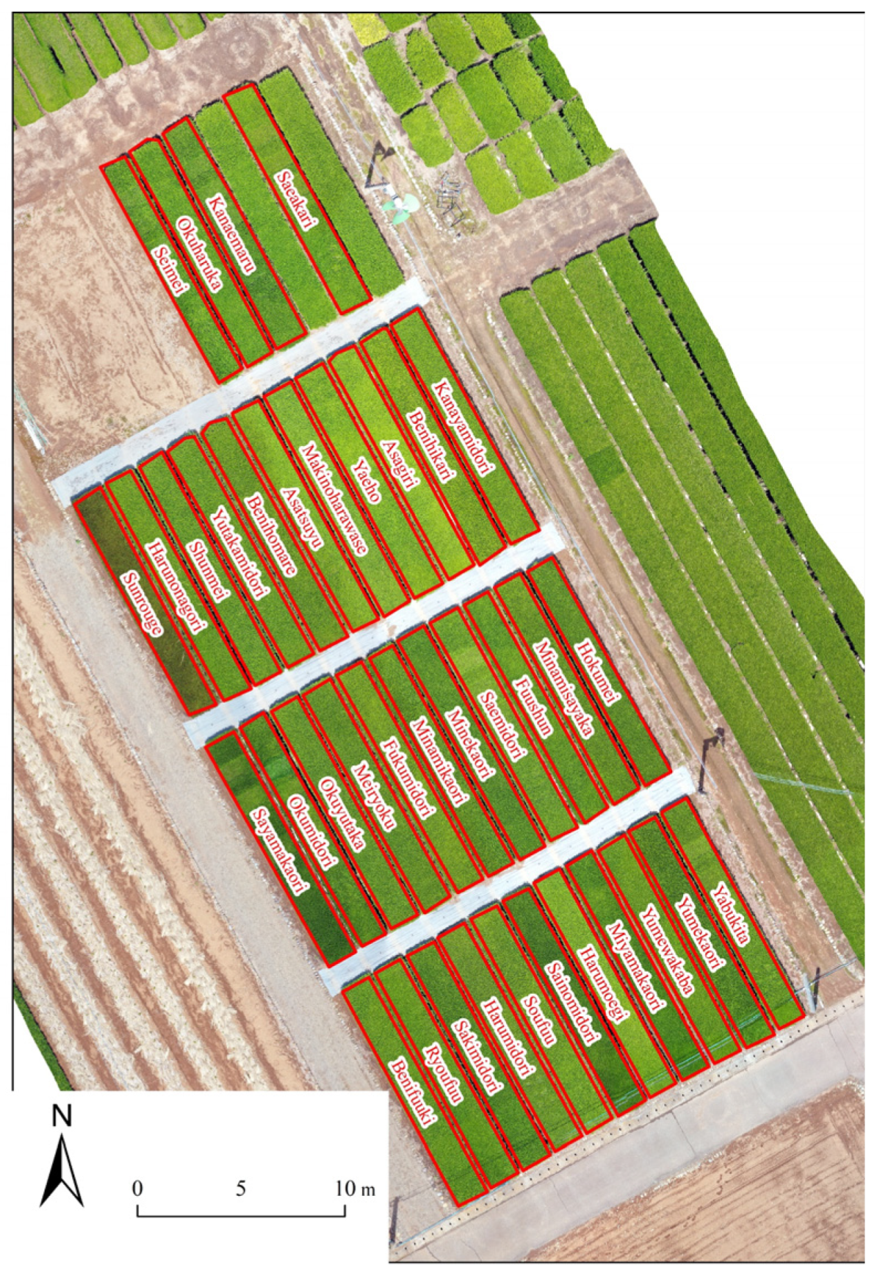
Figure 1. Aerial view of the tea field sampled in this study.
Remotesensing 15 00019 g001
Figure 2. Precipitation and sunshine duration: (a) on a monthly basis and (b) on an annual basis.
Remotesensing 15 00019 g002
Figure 3. The compact spectrometer and plant probe with a leaf clip used in this study.
Remotesensing 15 00019 g003
Figure 4. Third-leaf chlorophyll content of tea cultivars grown in this study.
Remotesensing 15 00019 g004
Figure 5. Correlations between chlorophyll content and a range of hyperspectral wavelengths when using various preprocessing techniques on the data.
Remotesensing 15 00019 g005
Figure 6. Frequency of selection for each wavelength based when using different variable selection methods and preprocessing techniques.
Remotesensing 15 00019 g006
Figure 7. Relationships between the ratio of performance to deviation (RPD) and root mean square error (RMSE) for each of the preprocessing and variable selection methods tested.
Remotesensing 15 00019 g007
Figure 8. Sensitivity analysis of regression models based on Cubist for DT preprocessing combined with the 14 variable selection methods.
Remotesensing 15 00019 g008
Table 1. Variable selection methods used in this study.
Filter method
Loading weights (LW)Regression coefficients (RC)Variable importance in projection (VIP)
Wrapper method
Backward variable elimination (BVE)Competitive adaptive reweighted sampling (CARS)Genetic algorithm (GA)
Iterative predictive weighting (IPW)PLS with Martens’ uncertainty test (MUT)Regularized elimination procedure (REP)
Sub-window permutation analysis (SwPA)Uninformative variable elimination (UVE)
Embedded method
Backward interval PLS (BiPLS)Forward interval PLS (FiPLS) Sparse PLS (SPLS)
Table 2. Software and packages used in this study.
Preprocessing/PLS RegressionPackage
First-derivative reflectance (FDR)prospectr [60]
Continuum removal (CR)prospectr [60]
De-trending (DT)prospectr [60]
Multiplicative scatter correction (MSC)mdatools [61]
Standard normal variate (SNV)prospectr [60]
Interval PLS (BiPLS and FiPLS)mdatools [61]
Sparse PLS (SPLS)spls [62]
CARSpracma [63]
Other PLSplsVarSel [64]
CubistCubist [57]
Table 3. Ratio of performance to deviation (RPD) for each regression model (100 repetitions).
MethodORFDRCRDTMSCSNV
BiPLS2.562.062.492.602.532.59
BVE2.532.072.552.502.442.49
CARS2.262.092.242.462.282.40
FiPLS2.411.992.472.592.492.52
GA1.751.571.831.991.912.07
IPW2.522.082.442.562.392.52
LWPLS2.451.952.462.502.272.55
Marten2.582.112.472.562.102.51
RC2.592.112.522.602.512.59
REP2.582.112.492.582.442.55
Sparse2.592.102.472.562.452.56
SwPA2.572.082.502.592.422.58
UVE2.051.582.002.362.072.22
VIP2.592.122.592.592.442.57
Table 4. Root mean square error (RMSE; μg cm−2) for each regression model (100 repetitions).
MethodORFDRCRDTMSCSNV
BiPLS3.274.073.363.223.313.23
BVE3.314.043.283.343.433.36
CARS3.714.013.743.413.673.49
FiPLS3.474.213.383.243.363.32
GA4.785.354.584.214.384.03
IPW3.324.033.433.273.513.32
LWPLS3.424.303.403.353.693.29
Marten3.243.973.393.273.993.33
RC3.243.963.323.213.343.23
REP3.243.973.363.243.433.28
Sparse3.233.983.393.273.423.26
SwPA3.264.033.353.233.463.25
UVE4.085.284.193.544.053.78
VIP3.233.953.243.233.433.25
Table 5. Optimal combinations of variable selection method and preprocessing technique after 100 repetitions.
Variable Selection MethodPre-Processing TechniqueTimeVariable Selection MethodPre-Processing TechniqueTime
BiPLSOR1RCOR3
BiPLSCR1RCCR2
BiPLSDT7RCDT8
BiPLSMSC4RCSNV2
BiPLSSNV3REPOR4
BVECR1REPDT1
FiPLSDT6SPLSOR4
FiPLSMSC1SPLSDT3
FiPLSSNV1SPLSMSC1
IPWOR3SPLSSNV3
IPWCR1SwPAOR2
IPWDT2SwPACR1
IPWSNV2SwPADT6
LWOR1SwPAMSC1
LWMSC2UVEOR1
LWSNV3UVECR3
MUTOR3UVEDT1
MUTCR3VIPCR5
MUTDT3VIPDT1
Disclaimer/Publisher’s Note: The statements, opinions and data contained in all publications are solely those of the individual author(s) and contributor(s) and not of MDPI and/or the editor(s). MDPI and/or the editor(s) disclaim responsibility for any injury to people or property resulting from any ideas, methods, instructions or products referred to in the content.