1. Introduction
Coastal dunes are natural landforms placed between the coastline and the hinterland that provide numerous ecosystem services to coastal areas. In particular, coastal dunes act as natural barriers that protect the hinterland from flooding [
1], provide habitat for numerous living species [
2,
3], and are natural sources of sand. This sand migrates to the shore during storms, mitigating beach erosion [
4].
In the last decades, coastal dunes have been subject to progressive degradation and loss [
4,
5,
6], with a consequent reduction of the ecosystem services they provide. A driver of coastal dune loss is overdevelopment [
4]. Since large areas along the coast are incorporated into the urban landscape (e.g., parking spots, walking pathways, roads, houses, etc.), they no longer protect the hinterland from waves and storm surges, causing coastal erosion [ibid.]. The impact of overdevelopment on dune survival was observed in Ravenna, Italy, where ~18 ha of coastal dunes have been lost in ~60 years due to the intensive construction of touristic establishments on the coastline [ibid.]. In the long term, coastal dunes loss will damage coastal structures, infrastructures, and ecosystems [
6] that are not protected by the dunes anymore. Another driver of dune loss is coastal erosion, which depends on wave action, sea-level rise (SLR), and frequency of storm surges [
7,
8], which are exacerbated by climate change [
9]. An example of dune erosion due to coastal hazards is the loss of the dune system on Galveston Island, Texas, in 1980, due to hurricane Allen [
1]. Since dunes did not yet recover when hurricane Alicia impacted the same area in 1983, storm surge dissipation was minimal [
10].
Numerical models have been extensively used to simulate the morphological evolution of coastal dunes. In particular, models have been used to simulate the morphological evolution of coastal dunes due to marine and aeolian forcings [
11,
12]. To obtain accurate results, the models require topographic (i.e., ground elevation) and ecological (i.e., vegetation height, density, and typology) information about the modeled environment. This data can be collected on the field using GPS-RTK and total stations, which are accurate but require excessive effort in both the collection and post-processing phases of the survey [
13]. For this reason, in the last decades, ground surveys have been progressively substituted by remote sensing, which is cheaper, more flexible, and less time-consuming [
14].
Among remote sensing techniques, unmanned aerial vehicles (UAVs) have been increasingly used to map coastal environments. The high revisit times enabled by low-cost UAVs make them valuable assets for monitoring highly dynamic coastal environments. UAVs are commonly used in combination with LIDAR (light detection and ranging) and SfM (structure from motion) techniques. LIDAR is a remote sensing technique that uses laser pulses to collect spatial data. UAV-based LIDARs are used to collect high-resolution point clouds, with densities often higher than 500 points m
−2 [
15]. UAV–LIDAR has been widely used to survey coastal areas [
16,
17,
18,
19], salt marshes [
20,
21,
22], grasslands [
23], and forests [
24,
25]. In vegetated areas, LIDARs have been used to determine both vegetation characteristics (i.e., canopy height and density) and ground elevation [
14,
23]. SfM photogrammetry (or Digital Aerial Photogrammetry, DAP) is a low-cost alternative to LIDAR to acquire point clouds [
26,
27]. In DAP, tridimensional point clouds are reconstructed by overlapping bidimensional images and using the distances between image key points [
28]. DAP has been widely used for agricultural mapping [
29], biological applications [
30,
31], as well as to survey salt marshes [
20,
21,
22] and coastal areas [
32]. DAP had also been combined with airborne LIDAR for coastal dune morphology evolution [
33]. DAP performances on ground elevation estimate are low in areas occupied by dense ad thick vegetation layers. This is because images do not contain sufficient details of the ground, due to the presence of vegetation, to perform image matching. Consequently, areas with taller and/or denser vegetation tend to have a lower number of points on the ground than unvegetated or less vegetated areas. For this reason, DAP is preferentially used to survey unvegetated areas, such as sandy beaches and dunes. Studies using UAV photogrammetry to monitor dune environments have focused more on the foredune or beaches than the back dune environment. For example, reference [
34] used UAV-photogrammetry to topographic monitor two areas, a beach and a sand spit, along the Portuguese coast.
Coastal areas present many challenges to ground elevation estimates with remote sensing techniques. In particular, it has been found that point cloud and ground elevation estimate accuracy decrease in topographically complex areas, with spatially variable or high slopes [
20,
21,
35,
36,
37,
38]. To overcome this limitation, reference [
21] recently introduced a procedure to transform the sloping-ground case into the flat-ground case. This was performed by approximating the real ground surface obtained from a point cloud by using a least-squares regression surface. The regression was based on the coordinates of the lowest points detected in the cells of the grid dividing the considered domain (a salt marsh system, in their case). Both a plane and a polynomial surface were used by [
21]. The regression plane gave better results on the marsh platform, reducing the error in the ground elevation estimate by ~25%. The polynomial surface instead, had better performance on the creeks, where the ground slope is higher. Here, the error in the ground estimate was reduced by ~40%. These results suggest that the application of the algorithm proposed by [
21] to topographically complex environments, such as coastal dunes, is essential to increase the accuracy of ground elevation estimates based on remote sensing techniques.
Several studies compared the performances of different survey techniques while used for beach dunes monitoring. For example, references [
37,
38] evaluate the applicability and limitations of terrestrial laser scanner (TLS) and UAV–DAP techniques to map beach-dune systems in northwestern Ireland and in Marina di Ravenna (Italy), respectively. They both found that TLS surveys produce more realistic surface models across beaches and sparsely vegetated areas. However, UAV–DAP should be preferred, since they can be used to survey larger areas in a certain time, compared to TLS, with similar accuracy. Moreover, they indicate that both techniques have lower performances in steep and vegetated areas. In addition, reference [
19] evaluated the applicability of three different point cloud generating methods, i.e., all terrain vehicles mounted mobile laser scan (ATV–MLS), airborne LIDAR, and UAV, to monitor beach surveys. They concluded that all point cloud techniques can be used to monitor coastal areas, but the choice of one of these techniques depends on several factors, such as funds availability, and the condition under which the system should operate. Additionally, reference [
17] compared UAV–LIDAR and UAV–DAP for beach monitoring. They indicate that UAV-LIDAR was the most suitable technique for performing beach surveys. However, this study has some limitations. First, the density of their UAV–LIDAR point cloud is limited to 60 points m
−2, which is generally observed for airborne point clouds. A consequence of this low resolution is the smaller likelihood of the point cloud to obtain data points at ground elevation below vegetated zones, which generally occupy a large portion of coastal dune areas. Second, that work does not consider the differences between UAV-LIDAR and UAV–DAP, in terms of the vertical distribution of the points of the point clouds, since they applied the same TIN-based filter to both datasets, to distinguish between ground and non-ground points, and then use the former to define the ground elevation surface. Finally, they did not take into account and remove the known negative effect of ground slope [
20,
21,
35,
36,
37,
38] on ground elevation estimate.
In this study, we use both a UAV–LIDAR and a UAV–DAP point cloud to determine the topography of a vegetated coastal area, comprehensive of back dunes, foredunes, and a freshwater forest, by using different regression techniques, i.e., multiple linear regression (MLR), genetic algorithm (GA), and random forest (RF). The study domain is a coastal dune environment located at Topsail Hill Preserve State Park in Santa Rosa Beach, Florida, USA. The LIDAR and DAP point clouds were collected using a custom UAS (unmanned aerial system) and are georeferenced using a total station and 12 ground control points (GCPs). To remove the effect of spatially variable and high slopes on ground elevation estimates, we applied the algorithm proposed by [
21] to both the UAV–LIDAR and UAV–DAP point clouds. In particular, the point clouds were transformed by using both the regression plane and polynomial surface methods, to evaluate their impact on the results. The three regression models are applied to both the UAV–LIDAR and UAV–DAP point clouds. The models are trained, validated, and tested through a rigorous Monte Carlo cross-validation procedure by using ground elevation data, which were manually collected using a RTK–GPS. Finally, we compared the ground elevation and the related estimation errors obtained from the cross-validated regression models.
2. Materials and Methods
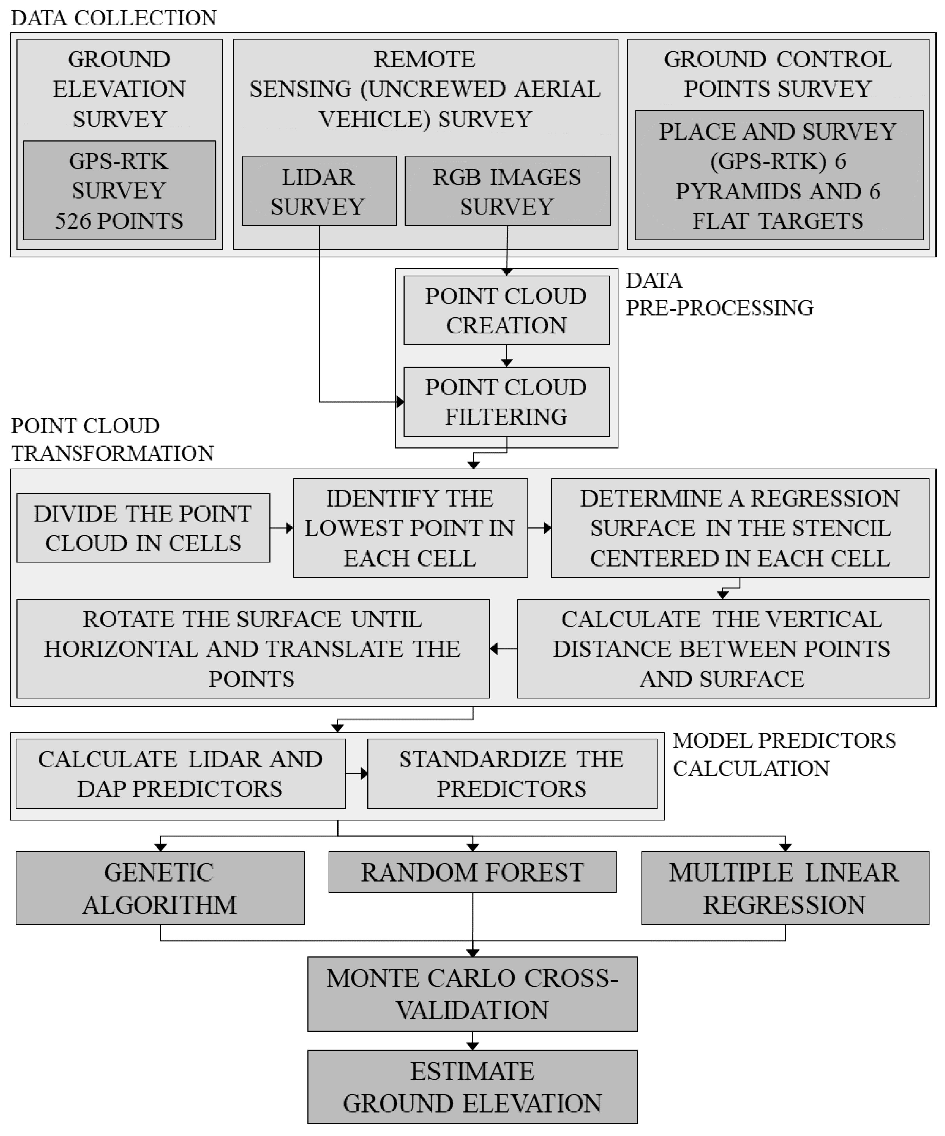
Our procedure consists of the following steps (reported in
Figure 1):
- STEP 1.
We performed a ground elevation survey on the field, by using a GNSS rover, to collect ground-truth data over our study domain (
Section 2.2).
- STEP 2.
We used a UAS to collect a high-resolution LIDAR point cloud and high-resolution RGB images over our study domain (
Section 2.3). We then calculated a DAP point cloud from the high-resolution images.
- STEP 3.
We transformed the UAV–LIDAR and UAV–DAP point clouds by using the method developed by [
21] to remove the effect of the ground slope on the ground elevation estimate (
Section 2.4.2).
- STEP 4.
We trained and tested three different regression techniques, a multiple linear regression, a genetic algorithm, and a random forest, to estimate the ground elevation from the transformed and the original point cloud (
Section 2.6). To train and test each technique, we performed a Monte Carlo cross-validation.
2.1. Study Site
The study domain is a ~0.5 km
2 coastal back dune environment located at Topsail Hill Preserve State Park (THPSP), located in Santa Rosa Beach, FL, USA (
Figure 2). The study domain is located southeast of Morris Lake and extends from the shoreline to the local coastal forest (
Figure 2b).
THPSP contains two large coastal dune lakes: Morris Lake and Campbell Lake. These lakes are a rare environment because they exchange water with a salty waterbody [
39]. The lakes are connected to the Gulf of Mexico through channels, which close off in dryer periods, and frequently change in appearance as the water creates new paths to the Gulf. In THPSP, water preferentially flows from the lakes to the Gulf of Mexico (i.e., outward, ibid.). However, specific wind conditions and tides invert the flow from the Gulf into the lakes (i.e., inward, ibid.).
THPSP is a unique brackish environment, which provides a habitat for a wide range of imperiled plant and animal species. This environment houses four subspecies of imperiled beach mice, three of which are endemic to the Florida Panhandle [
40]. In addition, the dunes provide a habitat for the gopher tortoise (
Gopherus polyphemus), as well as a nesting area for two rare shorebirds: the snowy plover (
Charadrius alexandrines) and Wilson’s plover (
Charadrius wilsonia, ibid.). Finally, the milkweed (
Asclepias humistrata, ibid.) that grows on the dunes is a key plant for the reproduction of migrating monarch butterflies (
Danaus plexippus, ibid.).
Apart from its ecological role, vegetation significantly affects the ability to map the area with remote sensing techniques. For example, it is documented that the ability to monitor exposed dunes in THPSP with remote sensing techniques is inhibited by plants growing on them, such as Gulf coast lupine (Lupinus westianus, ibid.).
2.2. Field Measurements
To perform the ground elevation survey, a plastic-capped iron rod was placed at the center of the survey area to serve as a semi-permanent monument. The Zephyr 3 base station was set up over this point and two Zephyr 3 GNSS rover units were used to collect checkpoints throughout the survey area. The expected accuracy is approximately 2 cm (RMSE). Measurements with the GNSS rovers were made using an observation time of 5 s. Results were processed using the projected coordinate system NAD 1983 UTM zone 16N.
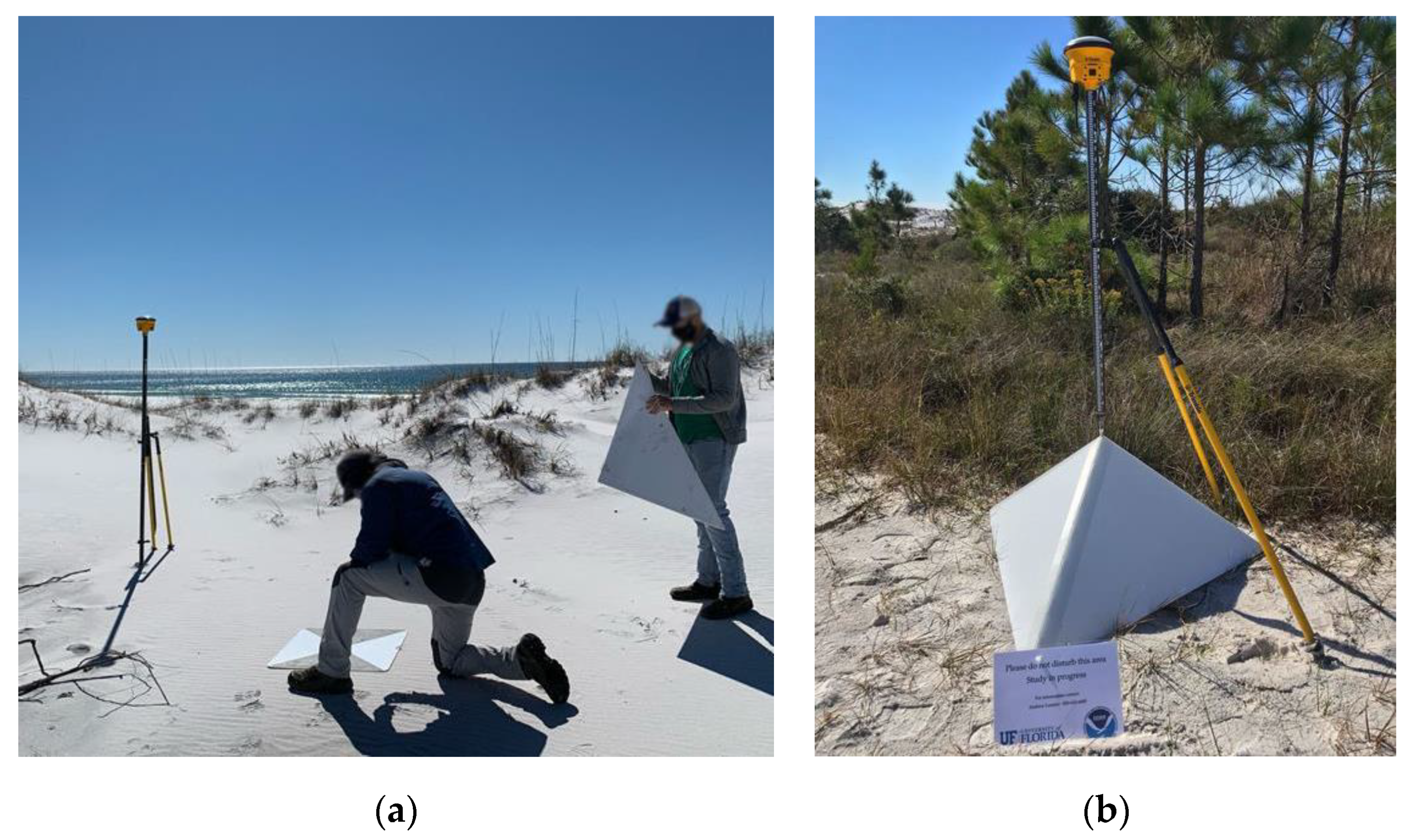
The complete survey included 526 checkpoints, 12 GCPs for the UAS survey (see
Section 2.3), and the location of the base station (light blue, orange, and violet markers, respectively, in
Figure 2b). The checkpoints were distributed in the study area to obtain measurements among different slopes and vegetation covers. Ground control points (GCP) were placed along two cross-shore transects separated by a longshore distance of ~500 m. Along each transect, pairs of GCP targets which consist of 1 flat target (
Figure 3a) and 1 pyramidal target (
Figure 3b), were set in three locations.
2.3. Remote Sensing Measurements
The UAS data collection was conducted using a Phoenix LIDAR Systems Scout-32 (Phoenix LiDAR System, Austin, TX, USA), which is a lightweight system that collects data at a range of up to 65 m. This system allows for the combination of multiple sensors, including a laser scanner and a variety of camera systems. For this collection, a Sony Alpha ILCE–A6000 CMOS (Sony Group Corp, Tokyo, Japan) was utilized in combination with the Velodyne HDL-32E laser scanner (Velodyne Lidar, San Jose, CA, USA). The Sony Alpha ILCE-A6000 is a 24-megapixel RGB camera with a complementary metal–oxide conductor sensor (CMOS). The Velodyne HDL-32E consists of 32 individual laser range finders which cover a field of view of 41.33 degrees parallel to the flight direction. The entire array of laser range finders continuously rotates providing a 360-degree field of view perpendicular to the flight direction. Each beam has a horizontal divergence of 2.79 mrad and a vertical beam divergence of 1.395 mrad resulting in a beam footprint of 8.3 cm × 4.1 cm at a range of 25 m. Each laser range finder can measure up to 2 returns per outgoing pulse, however, dual returns are registered only for objects separated by at least 1 m. The sensor can measure approximately 700,000 returns per second when operating in single-return mode. To collect our data, we used a flight altitude of 30 m and a line spacing of 25 m, respectively.
2.3.1. LIDAR Dataset
The UAV-LIDAR point cloud collected by using the Velodyne HDL-32E has an average density of ~1600 points m
−2. The geographic coordinates and the elevation of the points are assigned in the NAD 1983 UTM 16N geodetic system, and the WGS84 ellipsoid, respectively. The point cloud was adjusted by applying the procedure proposed in [
41] to the GCPs. The resulting residual in the target (GCPs) coordinates was ~1 cm.
2.3.2. Imagery Dataset
The Sony Alpha ILCE-A6000 CMOS camera was used to collect high-resolution images of the study area. The area contained in the RGB images is slightly smaller than the one surveyed for the LIDAR point cloud. The camera collected images from a nadir perspective, at the highest resolution (6000 × 4000 pixels), with a 3:2 aspect ratio. Images have a footprint of 45 m × 32 m, and an average overlap of 60%. We used the high-resolution RGB images as input for the Pix4DMapper software (Release 4.8.0, Pix4D, Prilly, Switzerland), to obtain a DAP point cloud. To georectify the images, the software uses a semi-automated approach, which requires manual identification of the GCPs in the input images. Thus, we identified the midpoint of each GCP in different groups of at least six images. The output DAP point cloud has an average point density of ~1200 points m
−2. The geographic coordinates and the elevation of the points are assigned in the NAD 1983 UTM 16N geodetic system, and the WGS84 ellipsoid, respectively. We compared the coordinates of the pyramidal GCPs centroids on the point cloud, with the corresponding values we surveyed in the field (see
Section 2.2). We obtained a horizontal and vertical georeferencing error of 2.8 ± 0.8 cm (mean absolute error ± root mean square error,
) and 3.2 ± 1.0 cm, respectively.
2.4. Ground Elevation Estimation
2.4.1. Point Clouds Filtering
We filtered both UAV-LIDAR and UAV–DAP point clouds by removing: (i) the points collected outside the study domain (red line in
Figure 2); (ii) the points which elevation is lower than 2 m below MSL; and (iii) the points whose elevation is higher than 20 m above MSL in the area occupied by the freshwater forest and 8 m above MSL along the coastline.
2.4.2. Point Cloud Transformation and Sloping Ground
In this study, we transform the UAV–LIDAR and UAV–DAP point clouds by applying the MATLAB algorithm proposed in [
21] to remove the effect of ground slope on the ground elevation estimate. The algorithm workflow is described in the
Supplementary Materials. In this section instead, we report only some relevant background from [
21].
The algorithm proposed in [
21] improves the estimate of ground elevation extracted from point clouds when the ground is sloping. Many approaches can be used to estimate the ground elevation distribution from a point cloud. Some of them use a classifier to distinguish between ground and non-ground points and then use the ground points to create a TIN surface that describes the ground elevation. Other methods are based on regular grids, in which the ground elevation is calculated for each cell as the minimum elevation of the point cloud contained in it, and assigned to the entire cell surface, or the cell center. For the latter, cell size must be large enough so that the chance that at least one of the points in the area describes the ground is sufficiently high and small enough so that the minimum elevation reasonably represents the elevation at its center. In addition, note that the survey points are not located at the center of a cell in the grid used to describe our study area. For this reason, their elevation was estimated by performing a bilinear interpolation on the elevation of the four cell centers surrounding each of the surveyed points. When tested on the 526 points we collected in the study area, we observed that the optimal average cell size corresponds to 30 cm for the point clouds.
For sloping ground, a point located in a less elevated region can be taken as the minimum and assigned to the cell center, producing large errors. To avoid this problem, the algorithm uses the point cloud contained in a 3 × 3 cells stencil (
), centered in the considered cell
(n,e), to estimate an approximation of the ground surface. This approximation is defined using a regression plane, or polynomial surface, based on the minimum elevations identified in the 9 cells constituting the stencil. The algorithm uses this approximation to transform a sloping-ground case into a flat-ground case (see
Supplementary Materials). In this study, cells are square and have a dimension of 30 cm × 30 cm.
The algorithm was applied to the UAV–LIDAR and UAV–DAP point clouds. The bed elevations were obtained from the techniques described in the next section, which use as inputs the predictors we calculated from the transformed and non-transformed point clouds, as described in
Section 2.4.3.
2.4.3. Model Predictors
This section summarizes the model predictors we computed by using the UAV–LIDAR and UAV–DAP point clouds in
. Each predictor was calculated for the non-transformed point clouds, as well as for the point clouds transformed using the planar and the polynomial regressions proposed in [
21] (see
Supplementary Materials). For readability, hereafter, we use the subscript “
n,e” to indicate the variables related to the stencil
.
The model predictors are:
The number of points of the point cloud contained in , .
The maximum elevation of the points in , :
where
is the elevation of the
point of the point cloud in
.
The mode elevation of the points in , . To calculate it, we divided the point cloud into six equivalent vertical layers, and we identified the mode as the average elevation of the layer containing the highest number of points.
The median elevation of the points in , . The value separates the higher and the lower halves of the points in . The value is unique if is an odd number. For even , there are two middle elevation values. We consider equal to their average.
The ground slope in
,
. The value is calculated as the maximum slope of the regression plane based on the minimum elevations identified in the 9 cells constituting the
(see
Section 2.4.2 and
Supplementary Materials).
The predictors are reported in
Table 1.
Finally, we standardized each predictor
using the following procedure:
where
,
and
are the standardized, the average, and the standard deviation value of the predictor
, respectively.
2.5. Regression Techniques
In the following sections, we describe the regression techniques we used in this study to estimate ground elevation from the UAV–LIDAR, and UAV–DAP transformed and non-transformed point clouds, by using the predictors reported in
Section 2.4.3. All regression techniques were implemented in MATLAB (release R2020b, MathWorks, Natick, MA, USA). The results obtained from each regression technique and point cloud will be compared by using the error metrics described in
Section 2.7.
2.5.1. Multiple Linear Regression
Multiple linear regression (MLR) is a statistical technique that uses multiple independent variables (i.e., predictors) to predict the outcome of a response (i.e., dependent) variable. These regressions are based on the following formula:
where for each observation
v,
is the dependent variable,
is the
of the
independent variables,
is the intercept on the ordinate’s axis,
is the slope coefficient associated to the
independent variable, and
is the model error.
Since MLR can have different performances based on the number of predictors used in the regression, we applied the regression to all the possible combinations of the predictors reported in
Table 1. The analysis was performed for all the point cloud types (i.e., UAV–LIDAR and UAV–DAP), and transformations (i.e., non-transformed, transformed plane, and transformed polynomial). The total number of combinations we analyzed is then equal to 4095.
2.5.2. Genetic Algorithm
To calculate ground elevation at each cell
(n,e), we used a regression model based on a genetic algorithm (GA). In the genetic algorithm, an initial population constituted of random entities changes until it reaches the optimal configuration, which resembles the configuration of a target population [
42]. This procedure simulates a biological evolution process, where the population evolves over consecutive generational steps. The individuals composing each step are chosen from those constituting the previous step by using a fitness function, which is calibrated on the target population.
In this study, the individuals are the model predictors calculated from the UAV–LIDAR and UAV–DAP point clouds, which are described in
Section 2.4.3 and are reported in
Table 1. The fitness function used to change the population at each stage is a linear regression function, which is used by the algorithm to fit the input data and was calibrated using the
. Finally, the target population is constituted of the GPS–RTK ground elevation points we collected in the study area.
Compared to traditional optimization algorithms, a genetic algorithm has many advantages [
43,
44], such as the possibility to be used with small datasets and to obtain as output an explicit equation for the ground elevation (i.e., our dependent variable) as a function of the model predictors. The formula can also be used to directly understand the relative importance of each predictor.
2.5.3. Random Forest Algorithm
To estimate the ground elevation in our study area, we also use a random forest (RF) regressor. A random forest is an ensemble-based machine-learning method that can be used for classification or regression problems. An ensemble method in machine learning employs multiple models to interpret given data and then combines the outcomes from each model to provide a result. In a random forest regressor, the model consists of a set of individual decision trees, operating as an ensemble. Given a dataset of labels (i.e., results, in our case, ground-truth elevation data collected in a survey) to use in the regression, each tree gives a prediction value to each label by using some regression features (i.e., the predictors). For each label, the average of the predictions produced by the trees is the prediction of the random forest regressor.
In this study, the dataset is constituted of the point clouds contained in each
. The regression features are the predictors calculated from the UAV–LIDAR and UAV–DAP point clouds, which are described in
Section 2.4.3 and reported in
Table 1. The predicted value is the ground elevation.
The model can be adjusted by determining the number of decision trees and the dimension of each tree [
45]. The performances of a random forest model might depend on the number of decision trees. To verify this, we made a sensitivity analysis. In the analysis, we trained the RF using 80% of the ground elevation points surveyed in the study domain (i.e., the cross-validation dataset described in
Section 2.6), and we tested it on the remaining 20% of the surveyed points (i.e., the test dataset described in
Section 2.6). The results indicate that the performance of the RF increases with the number of trees until they reach a stable value after ~2000 trees. For this reason, we used this value in our study. Finally, note that a high number of trees can significantly increase the computational cost of the model. However, because of the limited dimension of our dataset and the meager number of variables we considered, even a high number of trees does not significantly increase the computational cost of the model.
2.6. Training, Validation, and Testing of the Regression Techniques
We trained and tested the multiple linear regression, the genetic algorithm, and the random forest models by using a Monte Carlo cross-validation on the dataset of 526 RTK–GPS points we collected in our study domain (
Section 2.2). The dataset was divided into a cross-validation and a test dataset. They contain 416 and 110 entries, which correspond to ~80% and ~20%, of the entire dataset, respectively.
With the cross-validation dataset, we trained the algorithm using 333 entries (i.e., ~80%) randomly selected from the cross-validation dataset, we validated it on the remaining entries (i.e., ~20% of the cross-validation dataset), and we calculated the training and prediction errors. To perform the Monte Carlo cross-validation, we repeated this procedure 150 times (i.e., permutations). We then calculated the average training and validation error by averaging the errors obtained from each permutation, and we used them to verify the performances of the model during the training and validation steps. Once the model is validated, we tested it on the test dataset. Once the model is tested, we used the whole 526-entities dataset to determine the regression formulas and calculate the ground elevation. This procedure is performed for each model by using MATLAB.
2.7. Error Analysis
We quantified the error of the estimated ground elevation by using the
, the
, and the coefficient of determination (
). The considered model has good predictive skills if the value of
and
are close to zero, and if the value of
is close to 1. The value of the error metrics was calculated as follows:
In Equations (11)–(13), yo and ypr are the observed and predicted quantities, respectively, in the sampling location, and is the dimension of the dataset.
5. Conclusions
In this study, we compared the results obtained by applying different regression techniques (i.e., multiple linear regression, genetic algorithm, and random forest), to a UAV–LIDAR and a UAV–DAP point cloud, to estimate the ground elevation in a coastal environment. The results are validated using a robust Monte Carlo cross-validation.
Our study is the first one that compares the performances of UAV–LIDAR and UAV–DAP point clouds when they are used to estimate topographic features in a coastal environment dominated by coastal dunes, and that reduces the error caused by a sloping terrain. Previous studies perform this comparison in forests, salt marshes, and grasslands, or use low-resolution point clouds, collected from aircraft and satellites. The results we obtained underline the pro and cons of UAV–LIDAR and UAV–DAP methods in this environment. Thus, this study can help both scientists and local managers to choose a survey method, depending on their budget and the desired quality of their results.
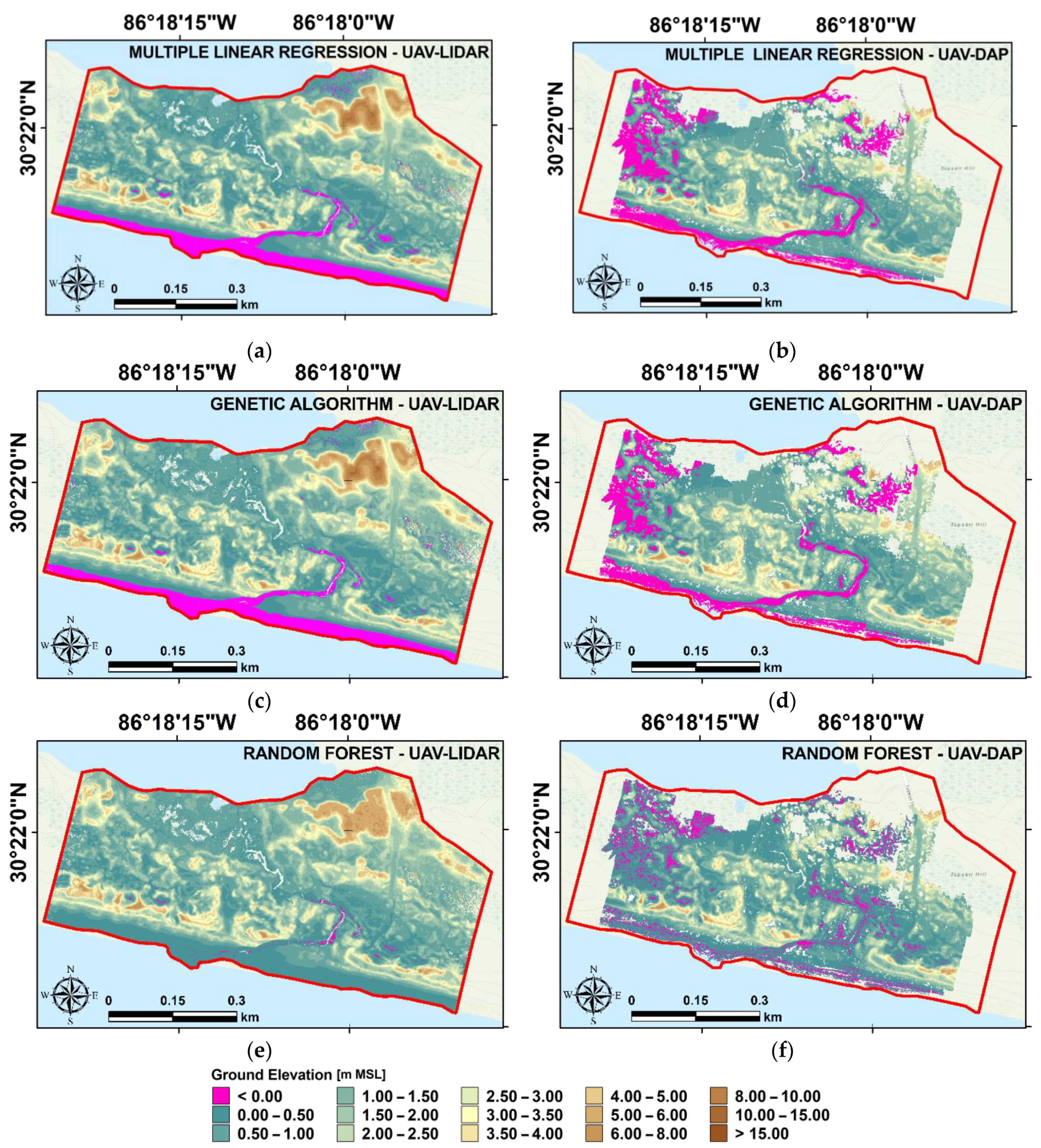
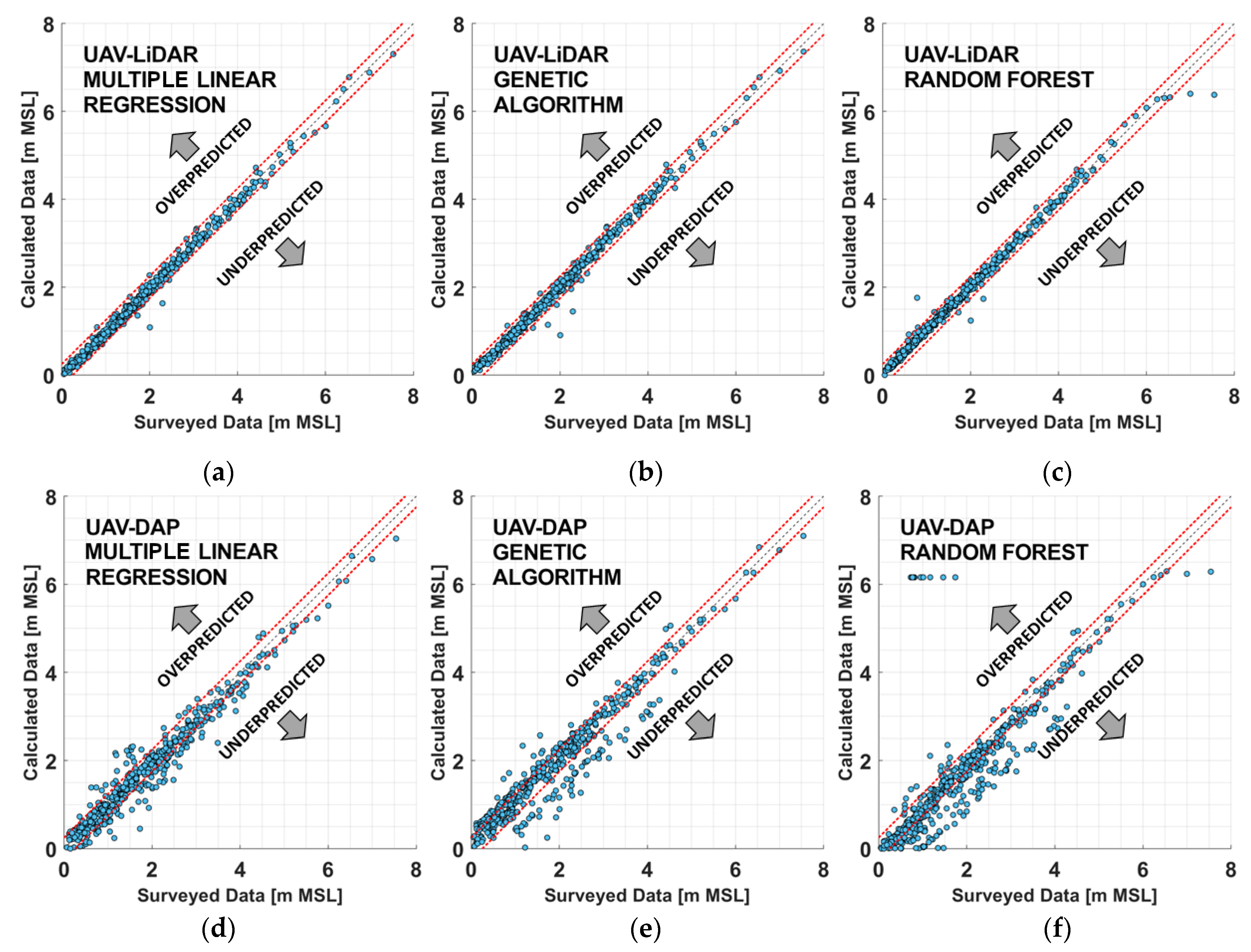
The results suggest that the UAV–LIDAR datasets should be preferred to the UAV–DAP datasets to estimate ground elevation in the considered coastal area. This is because of the lower estimation error obtained by using the LIDAR point cloud. The high estimation error obtained using the UAV–DAP point clouds is due to the limited capability of photogrammetry to acquire information below vegetation layers, and thus to the limited capability to determine elevation points close to the real ground level during the transformation of the imagery dataset in a appoint cloud.
Our study is also the first one comparing different regression techniques to estimate ground elevation in a coastal environment dominated by coastal dunes from high-resolution point clouds. The results suggest that optimal and similar results can be obtained from both the genetic algorithm and multiple linear regression, and that, for this reason, they should be preferred to random forest to estimate ground elevation. These results are independent of the point cloud (i.e., UAV–LIDAR or UAV–DAP) used to calculate ground elevation, and on the pre-processing geometric transformation performed on them.
To conclude, the results suggest that the most accurate description of ground elevation in our study area was obtained by applying the genetic algorithm to a point cloud transformed using a regression plane. For this reason, we suggest the use of this combination of techniques to describe the topography in similar coastal environments.
Future works will focus on the identification of the vegetation properties, such as height, density, and species, in the study area, by using a combination of imagery and LIDAR data. This will be beneficial to investigate the temporal and spatial modification of these properties. For example, the migration of the freshwater forest can be used as a proxy to estimate saltwater intrusion or the impact of SLR. Vegetation loss can also be used to estimate the impact of natural hazards on the coastline. Climate changes and natural hazards have an important effect also on the local topography. For instance, in our study area, storm surges, hurricanes, and SLR can modify the path of the tidal creek connecting Morris Lake and the Gulf of Mexico. These modifications will impact not only the local topography but also the vegetation. Coastal hazards can cause dune breaches, and consequently coastal floodings, which can impact the local coastal communities. For this reason, future works will focus on the identification of topographic modification by using only LIDAR point clouds, as suggested by our results.
Finally, we underline that, in this study, we used a raster, instead of a TIN surface to describe the ground elevation for two reasons. First, we wanted to divide the point cloud into comparable subsamples, made of a similar number of points. This was performed to avoid the possible effect of sample size in the computation of the predictors we used in the regressors (i.e., RF, MLR, and GA) to compute the ground elevation. Second, by considering only the lowest elevation point in each cell of a raster, we employed a slope correction method that uses the nine points in a three cell × three cell stencil everywhere, to estimate the ground elevation. This method, based on a least square error procedure, is simple and relatively fast. On the contrary, if we had used more than one point per cell, the least square error correction method on each node of a TIN would use a larger number of points at each location, at the cost of computational time. Moreover, it is unclear if more points would increase or decrease the accuracy. To improve the computational speed, a subset of these points can be selected. However, it is uncertain how to select the points of this subset. For these reasons, future works will focus on the use of a point cloud transformation method based on the ground slope calculated on a TIN surface to describe the ground elevation in coastal areas.


