Abstract
Mesoscale eddies have essential effects on the distribution of the different sizes of phytoplankton and the status of phytoplankton physiology. The impact of mesoscale eddies on phytoplankton size and physiological level in the northern South China Sea is analyzed based on satellite data and HYCOM-simulated results from 2003 to 2018. The results show that there are higher nanophytoplankton levels for high and low nonlinearity in the center of cyclonic eddies. At the same time, the growth rate of phytoplankton increased, and the assimilation of phytoplankton decreased. Moreover, in the center of anticyclonic eddies, a lower nanophytoplankton level is observed in both high and low nonlinearity. At the same time, the growth rate of phytoplankton decreased, and the assimilation of phytoplankton increased. In addition, there is a higher nanophytoplankton level in the mode-water eddy, while the growth rate of phytoplankton is increased, and the assimilation of phytoplankton is decreased.
1. Introduction
Phytoplankton patterns influenced by mesoscale eddy dynamics can be frequently detected by satellites. The physical mechanisms responsible for phytoplankton variability in mesoscale eddies are still hotly debated [1,2]. The main mechanisms of eddy-driven phytoplankton variability include vertical effects such as eddy pumping, eddy-wind interactions, and eddy impacts on the mixed-layer depth and horizontal effects, such as eddy stirring and eddy trapping [3]. The former mechanisms can regulate the vertical distribution of nutrients or light availability to affect phytoplankton productivity. Moreover, the latter can only advect water masses around the eddy and is not expected to have a biogeochemical effect [4]. Eddy pumping-induced shallowing (deepening) of the mixed layer in cyclonic (anticyclonic) eddies uplifts (depresses) the nutricline closer (further) to the euphotic zone and increases (limits) nutrients available for photosynthesis [5,6]. On the other hand, the wind-driven Ekman current interacts with the cyclonic (anticyclonic) eddy and generates convergence (divergence) inside the eddy, resulting in a high phytoplankton biomass. The chlorophyll anomalies driven by eddy pumping, eddy-wind interactions, and eddy-induced variability of the mixed layer depth appear as a monopole structure in the center of the eddies [7,8]. Biological activities associated with anticyclonic eddies are more complex than those associated with cyclonic eddies [9]. Ring-shaped pattern chlorophyll anomalies typically occur at the peripheries of anticyclonic eddies with large horizontal density gradients, strains, and vertical velocities, containing more complex biological activities [10,11]. The possible mechanism of the ring-shaped pattern is the increase in nutrients caused by nutrient-rich water transport upward along the up-bowed isopycnals at the periphery of eddies, or the addition of nutrients caused by upwelling at the periphery of anticyclonic eddies. This simulates phytoplankton growth [12,13,14].
The South China Sea (SCS) is the largest marginal basin connected to the western Pacific Ocean, with a total area of 3.5 million km2 and an average depth of greater than 3000 m. The SCS is oligotrophic with limited nitrogen and phosphorus within the euphotic layer. In the northern SCS, there is a meridional gradient of chlorophyll due to differences in nitrogen between the north and the south [15,16]. The Northern South China Sea (NSCS) is the dynamically active region in the SCS. Mesoscale eddies are ubiquitous and generated in the NSCS, often propagating westward and slightly inclining to the south, near the continental slope. Previous studies have shown that the main eddy mechanisms affecting phytoplankton include eddy pumping, interactions between wind and eddies, and advection in the NSCS. Low chlorophyll concentrations caused by eddy pumping are often observed in the center of anticyclonic eddies [17]. The interactions between wind and eddies cause the anticyclonic pattern to change. When the anticyclonic pattern is extended parallel to the South China Sea wind direction, eddy-induced Ekman pumping will induce high concentrations of chlorophyll [18]. An anticyclone formed near the coastal area of the NSCS can capture high chlorophyll water and transport it to the oligotrophic region of the NSCS [19].
However, the impact on the sizes of phytoplankton due to mesoscale eddies has been sparsely researched. The distribution of diatoms in the small space is very heterogeneous, especially for mesoscale eddies and submesoscale fronts. Eddies show either enhanced or reduced abundances in eddy cores [20]. The enhanced productivity in an eddy near the Luzon Strait shed from the Kuroshio Current was comparable to wintertime productivity in the SCS basin, which is supported by upwelled subsurface nitrate under the prevailing Northeastern Monsoon. There were more Synechococcus, picoeukaryotes, and diatoms, but less Trichodesmium in the surface water inside the eddy than outside [21]. Phytoplankton in a cold-core eddy with low surface iron concentrations have been shown recently to upregulate iron uptake and utilize iron from enhanced microbially mediated recycling, which has large-scale importance in influencing phytoplankton dynamics under climate change [22,23]. Moreover, the mode-water eddy, which has the same positive sea level anomaly signal as the anticyclonic eddy detected from the altimeter, but whose chlorophyll increases abnormally at the eddy’s core, has been less studied. The seasonal pycnocline is uplifted in the mode-water eddy, while the seasonal pycnocline is compressed in the anticyclonic eddy. McGillicuddy et al. found that some anticyclonic eddies in the sea area are mode-water eddies with a lens-shaped internal pycnocline structure and high chlorophyll values in the surface layer [24]. Barceló-Llull et al. found a mode-water eddy in the scientific voyage of the eastern boundary upwelling system region [25]. They found that the mode-water eddy is similar to the cyclonic eddy and is different from the anticyclonic eddy, which brings cold, low-salinity water to the surface. Most of the studies only studied the effect of a single eddy on phytoplankton size. Analyses of the effects of multiple eddies on phytoplankton size over large areas are lacking.
2. Data and Method
2.1. Satellite and Model Data
The study area for the mesoscale eddy analysis covered the area from 15°N–23°N and 110°E–120°E, which is also defined as NSCS by Liu et al. (2013). The sea surface level anomaly (SLA) and geostrophic velocity data that we used to cover approximately sixteen years from 2003 to 2018 were extracted from the Delayed-Time Reference Series provided by Archiving, Validation, and Interpretation of Satellite Data in Oceanography (AVISO). The data were gridded to 1/4° × 1/4° with a time step of 7 days. The SLA data were high-pass filtered spatially with half-power filter cutoffs of 20° longitude by 10° latitude over the global ocean. This spatial high-pass filtering attenuates SLA variability associated with large-scale Rossby waves and removes steric heating and cooling effects.
An algorithm was created based on empirical orthogonal functions (EOFs) for globally retrieving the chlorophyll-a concentration (Chl-a) of phytoplankton size classes (PSC) with microplankton, nanoplankton, and picoplankton from multisensor merged ocean color (OC) products. The data were gridded to 4 km × 4 km with a time step of 1 day and were extracted from the Copernicus Monitoring Environment Marine Service (CMEMS) [26]. We also use particulate organic carbon (POC) and Chl-a data from GlobColor [27]. The original NASA algorithm with correlations of band ratios was used to retrieve POC concentration data [28]. The Chl-a concentration for case 1 water is merged by all sensor data using Maritorena’s method [27].
In order to verify the applicability of satellite products in the South China Sea, this paper uses the HPLC measured data of four cruises in the SEABASS database (https://seabass.gsfc.nasa.gov/, accessed on 24 December 2022) for verification. Finally, 10 coincident satellite data and HPLC data were selected at near-surface depths (<10 m) using the nearest method, as show in Figure 1. The time range includes 2009, 2011, 2013, and 2016.
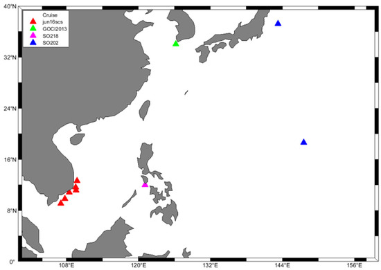
Figure 1.
Locations of 10 in situ HPLC and satellite data, with the cruise name displayed in the legend.
To further explore the effect of eddies on phytoplankton, this paper uses the VGPM model to calculate primary productivity (PP) [29]. Yoshie et al. calculated PP/Chl to express the carbon sequestration efficiency per unit of chlorophyll in phytoplankton and calculated PP/POC to express the growth efficiency of phytoplankton [30].
To minimize the effects of data gaps and cloud contamination in the daily image, the ecological data at each grid box were low-pass filtered in time using a loess smoothing filter with a half-power cutoff of 30 days. The ecological data were then low-pass filtered in space with 2° × 2°, similar to the smoothing procedure used to construct the AVISO ‘s SLA fields. This low-pass spatial filtering removed sudden, local phytoplankton bloom events. The remaining data gaps were completed using kriging interpolation. The ecological data were also high-pass filtered zonally to attenuate the zonal wavelength scales larger than 20° in longitude. To attenuate both the large-scale and seasonal variability of the phytoplankton size data, the ecological data were high-pass filtered at 6° × 6° and 500 days. Similar to SLA, after preprocessing, the results in the NSCS were also extracted from global data [12,29]. We only considered the mesoscale eddies in the water depth area of more than 200 m. The PSC data at depths shallower than 200 m were also removed [15].
HYCOM is a hydrostatic, primitive equation general circulation model that evolved from the Miami Isopycnic Coordinate Model (MICOM). Its general architecture and initial validation are documented by Bleck [31], followed by further developments by Halliwell [32]. Flexible options for the vertical grid enable HYCOM to conserve water mass properties in isopycnal coordinates when there is strong vertical stratification and provide adequate vertical resolution in regions with weak stratification, such as the surface mixed layer. This study uses HYCOM’s temperature and salinity to calculate the anomaly data, where the anomaly data were equal to the initial value minus the climatological value. The quasi-geostrophic vertical velocity is obtained from OMEGA3D model data. The quasi-geostrophic vertical velocity anomaly is obtained by subtracting the climatological average from the quasi-geostrophic vertical velocity.
2.2. Calculations and Methods
To identify the three size classes (micro, nano, and pico) and quantify their relative mproportions, Vidussi et al. [33] selected seven major pigments as diagnostic pigments (DP) for distinct phytoplankton groups. These seven pigments are fucoxanthin (Fuco), peridinin (Perid), 19′ = hexanoyloxyfucoxanthin (Hex-Fuco), 19′-butanoyloxyfucoxanthin (But-Fuco), alloxanthin (Allo), chlorophyll b (Chl b), and zeaxanthin (Zea). Because some taxonomic pigments might be shared by various phytoplankton groups, Uitz et al. [34] combined the multiple regression approach of Gieskees et al. [35] to determine the weight of seven pigments in chlorophyll-a, , according to
The fractions of the chlorophyll-a concentration associated with each of the three size classes are subsequently derived according to
The actual chlorophyll a concentration associated with each of three size classes is derived according to
As the distribution frequency of each phytoplankton group was left-skewed, we log-transformed them to log10 to satisfy a roughly normal distribution.
The model prediction accuracy was evaluated by several statistical parameters: (1) coefficient of determination (R2), and (2) root mean squared error (RMSE). According to Equations (8)–(11), respectively:
where SST is the sum of square due to error (SSE) and the total sum of square (SST), yi is the true value in sample I, yi′ is the predicted value in sample i, and is the average of the true values.
We identified and tracked mesoscale eddies using a sea surface height-based method developed by Chelton et al. [36]. The method worked as follows: anticyclonic and cyclonic eddies are defined separately. When a anticyclonic eddy was identified, the SLA was partitioned starting from a SLA threshold of −100 cm and proceeded upwards in increments of 1 cm until a closed SLA contour was achieved, that satisfied the following criteria: (1) the SLA value of all of the pixels in the closed SLA contour were above the SLA threshold; (2) at least 8 pixels and fewer than 1000 pixels were enclosed by the closed contour of SLA; (3) there was at least one local SLA maximum; (4) the amplitude of the eddy was at least 1 cm; and (5) the maximum distance between any pairs of points within the closed SLA contour must be less than a specified maximum to exclude the irregular shaped eddies. Chelton et al. have taken the specified maximum to 400 km for latitudes above 25°, and the maximum distance criterion was increased linearly to 1200 km at the equator. The cyclonic eddy is similarly identified, with the thresholding beginning at 100 cm, and proceeding downwards. This procedure is also satisfied the five eddy definition criteria, with the criteria (1) is that the SLA value of all of the pixels in the closed SLA contour were below the SLA threshold; criteria (3) is that there was at least one local SLA minimum; criteria (4) is that the amplitude of the eddy was at most −1 cm; and criteria (2) and (5) is the same as the anticyclonic eddy’s criteria (2) and (5).
The identification method of mode-water eddies is as follows. Studies on mode-water eddies show that compared with anticyclonic eddies, mode-water eddies have a similar shape to the anticyclonic eddies at the SLA. However, the mode-water eddies have negative temperature anomalies and negative salinity anomalies at the center [25,37]. Therefore, this paper makes a simple modification based on Chelton’s method to identify mode-water eddies: if the temperature and salinity anomaly at the center of the anticyclonic eddy is less than 0, then this anticyclonic eddy is regarded as a mode-water eddy. The flowchart of the identification method of mesoscale eddies is shown in Figure 2.
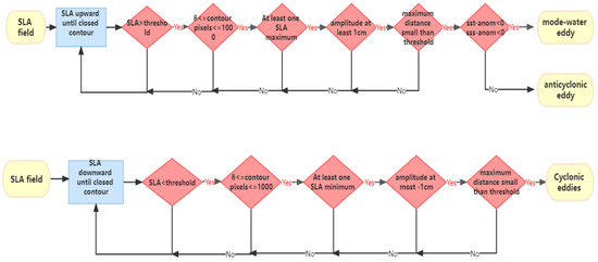
Figure 2.
The flowchart of the identification method of mesoscale eddies.
The properties of each eddy were calculated as follow: the eddy scale (Ls) is defined by the radius of the circle having the same area as the closed contour of the SLA with the maximum mean geostrophic current speed; the amplitude of the eddy (A) is defined by the height difference between the eddy periphery and centroid. The rotation speed U is estimated by
where g is the gravitational acceleration and f is the Coriolis parameter. The eddy kinetic energy (EKE) is the energy associated with the turbulent part of the flow of a fluid. It is calculated by
where uag and vag are the geostrophic velocity anomalies. Finally, the nonlinear degree was defined as the ratio of the rotation speed (U) to the translation speed (c), which was estimated from the distance traveled by the eddy centroid and the time interval between the two adjacent positions of the centroid. The nonlinear degree represents the potential to trap water parcels in the eddy’s interior. For highly nonlinear eddies (higher ratios), it is more difficult for water parcels to escape from the eddy interior [36]. Hence, nonlinear eddies have essential effects on marine ecosystem dynamics. Only nonlinear eddies (U/c > 1) were considered in this study. Low nonlinear eddies are defined as eddies with nonlinear degree of more than 1, but less than 10; high nonlinear eddies are defined as eddies with nonlinear degree of more than 10.
The composing analysis was defined as composing the region within a circle centered at the eddy centroid and twice the eddy scale Ls. Composite values were calculated by averaging the time series at each rotated and horizontally normalized location within a radial distance of 2Ls from the eddy centroid.
Siegel et al. pointed out that chlorophyll’s monopole structure reflects mesoscale eddies’ role in addition to eddy stirring, and the dipole structure reflects the role of eddy stirring in a mesoscale eddy [4]. Gaube et al. simulated the monopole and dipole structures of chlorophyll anomalies and combined them. The results were similar to the anticyclonic eddy observed in the Leeuwin Current [7]. Frenger et al. separated unipolar SST anomalies by radially averaging the total SST anomalies relative to the eddy’s centroid [23]. A method is used to separate monopoles and dipoles in mesoscale eddies; subtract the remaining term of the monopole structure from the synthetic mean data of the mesoscale eddies as the dipole structure of the mesoscale eddies. The specific formula is
where r is the eddy radius and is the rotational angle. The overbar denotes the radial average, and the prime denotes the residuals [7]. Figure 3 shows the composites of a CHL monopole and a CHL dipole.
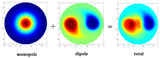
Figure 3.
Composites of a CHL monopole and a CHL dipole.
3. Results
3.1. The Validation of PSC Satellite Data in the SCS
In this paper, we use 10 HPLC measured data to verify the applicability of the PSC satellite data in South China Sea. These data are obtained from the SEABASS database and come from four cruises. As a result, in Figure 4, the satellite data is fitted with the in-situ data (R2 > 0.5). However, due to the lack of on-site data and the influence of remote sensing data on weather and other factors, only 10 sites could be found during the four cruises, while satisfying the match between the measured data and the remote sensing data.
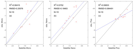
Figure 4.
Scatter plots of in−situ versus satellite data: (a) micro, (b) nano, and (c) pico. The solid line is the trendline, and the dotted line is the 1:1 line. The N is the number of samples.
3.2. Distribution and Characteristics of Mesoscale Eddies in the Northern South China Sea
The trajectories of different mesoscale eddies in the northern South China Sea are shown in Figure 5. Figure 5a shows that the anticyclonic eddies in the northern South China Sea are mainly generated on the eastern side of the northern South China Sea and gather on the southwestern part of Taiwan Island and the western side of Luzon Island. The eddy trajectories of the anticyclonic eddy spread almost all over the NSCS. The number of anticyclonic eddy trajectories in summer is 94, and the number of anticyclonic eddy trajectories in winter is 83. The number of anticyclonic eddies in the NSCS is greater in summer than in winter. In the NSCS, the anticyclonic eddies move mainly westward and incline southward along the continental shelf. Figure 5b shows that cyclonic eddies in the northern South China Sea are mainly generated in the northern South China Sea and mainly gather on Luzon Island’s west side. The eddy trajectories of the cyclonic eddy are almost all over the NSCS. The number of cyclonic eddy trajectories in summer is 118, and the number of cyclonic eddy trajectories in winter is 133. The number of cyclonic eddies in the NSCS is more significant in winter than in summer. From the total number of eddies, the number of winter mesoscale eddies in the northern South China Sea is higher than that of summer mesoscale eddies. Figure 5c shows that the number of mode-water eddies in the NSCS is scarce, with three mode-water eddy trajectories in winter and six mode-water eddy trajectories in summer. The mode-water eddies are not always in the northern South China Sea, and the number of mode-water eddies in summer is higher than that in winter.
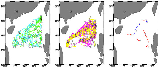
Figure 5.
(a) The eddy trajectories of the anticyclonic eddy. Cyan trajectories are the eddy trajectories in winter. Green trajectories are the eddy trajectories in summer. (b) The eddy trajectories of the cyclonic eddy. Yellow trajectories are the eddy trajectories in winter; pink trajectories of the cyclonic eddies in summer; (c) eddy trajectories of the mode-water eddy. Blue trajectories are the trajectories of the mode-water eddy in winter, and red trajectories are the trajectories of the mode-water eddy in summer.
Table 1 summarizes the characteristics of different mesoscale eddies. In the northern South China Sea, 177, 251, and 9 eddy trajectories of anticyclonic, cyclonic, and mode-water eddies correspond to 996, 1460, and 27 eddies, respectively. Among them, the numbers of anticyclonic eddies, cyclonic eddies, and mode-water eddies are 361, 420, and 5 in summer, respectively, and the numbers of anticyclonic eddies, cyclonic eddies, and mode-water eddies in winter are 635, 1040, and 22, respectively. The numbers of high nonlinear anticyclonic and cyclonic eddies are 12 and 21, respectively, and the mode-water eddies have no high nonlinear eddies. The numbers of low nonlinear anticyclonic, cyclonic, and mode-water eddies are 359, 610, and 12, respectively. The average eddy amplitudes of the anticyclonic eddy, cyclonic eddy, and mode-water eddy are 14.07 cm, 13.02 cm, and 13.09 cm, respectively. The average rotating speeds are 0.149 m/s, 0.138 m/s, and 0.159 m/s, respectively. The average transmission speeds are 0.058 m/s, 0.064 m/s, and 0.053 m/s, respectively. The average effective radii are 134.37 km, 136.43 km, and 126.28 km, respectively. The ratios of nonlinear mesoscale eddies (U/c > 1) to all eddies are 31.32%, 31.28%, and 27.91% of the total number of anticyclonic, cyclonic, and mode-water eddies, respectively. The average nonlinearities of anticyclonic, cyclonic, and mode-water eddies are 2.90, 2.77, and 1.49, respectively.

Table 1.
Statistical data of various eddies in the NSCS (S. means summer, W. means winter.).
3.3. Monopole Distribution of Phytoplankton Size and Physiological Characteristics inside Mesoscale Eddies
Figure 6 shows that in cyclonic eddy monopole decomposition, the phytoplankton of each size in the center of the eddy increased, the increase in phytoplankton gradually decreased with increasing distance from the center, and there was a slight decrease in phytoplankton at the periphery of the eddy. Comparing the low nonlinear cyclonic eddy and the high nonlinear cyclonic eddy in the monopole image, the increase in phytoplankton in the center of the low nonlinear cyclonic eddy is less than the increase in phytoplankton in the center of the high nonlinear cyclonic eddy. The reduction in phytoplankton at the periphery in a low nonlinear cyclonic eddy is less than that of phytoplankton at the periphery in a high nonlinear cyclonic eddy. The reduction in phytoplankton at the periphery of the cyclonic eddy was much smaller than the increase in the eddy’s center. Comparing the variations in phytoplankton of different sizes in the cyclonic eddy, the increase in phytoplankton in the center of the cyclonic eddy was in the order of nanophytoplankton > microplankton > picophytoplankton. The reduction in phytoplankton of each size at the periphery of the eddy was similar and much smaller than the increase in the eddy’s center.
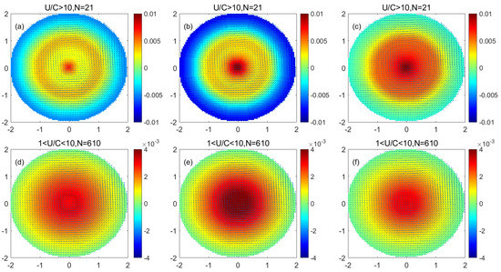
Figure 6.
(a–c) are the monopole distribution of microplankton, nanophytoplankton, and picophytoplankton in the high nonlinear cyclonic eddy, respectively; (d–f) are the monopole distribution of microplankton, nanophytoplankton and picophytoplankton in the low nonlinear cyclonic eddy, respectively. (Unit: mg/m3).
Figure 7 shows that in the monopole decomposition of the cyclonic eddy, both PP and POC increase in the center of the eddy, and the increase in PP and POC in the eddy gradually decreases with the distance from the center of the eddy. PP and POC concentrations decreased at the periphery of the eddy. The value of PP/Chl in the center of the cyclonic monopole is low, indicating that the carbon sequestration efficiency of phytoplankton unit chlorophyll in the center of the cyclonic eddy is low. The value of PP/POC in the center of the cyclonic monopole is high, indicating that in the cyclonic eddy, there is increased efficiency with which phytoplankton produces new productivity. Comparing the physiological status of the high nonlinear cyclonic eddy and the low nonlinear cyclonic eddy, it can be found that the increases in PP, POC, and PP/POC in the high nonlinear cyclonic eddy are more significant than those in the low nonlinear cyclonic eddy. With the increase in PP, POC, and PP/POC in the nonlinear cyclonic eddy, the PP/Chl of the high nonlinear eddy is smaller than the PP/Chl of the low nonlinear eddy. This shows that the vertical and horizontal effects of high nonlinear cyclonic eddies have more significant effects on the physiological status of the eddy than the vertical effect of low nonlinear cyclonic eddies.
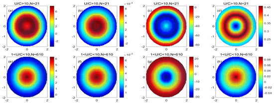
Figure 7.
(a–d) are the monopole distribution of the PP variation, POC variation, PP/Chl, and PP/POC in a high nonlinear cyclonic eddy, respectively; (e–h) are the monopole decomposition of the PP variation, POC variation, PP/Chl, and PP/POC in a low nonlinear cyclonic eddy, respectively. (Unit: mg/m3).
Figure 8 shows that in the monopole decomposition of the anticyclonic eddy, the phytoplankton of each size in the center of the eddy decreased, the decrease in phytoplankton gradually decreased with increasing distance from the center, and there was an increase in phytoplankton at the periphery of the eddy. Comparing the low nonlinear anticyclonic eddy and the high nonlinear anticyclonic eddy, the phytoplankton reduction in the center of the low nonlinear anticyclonic eddy is less than that in the center of the high nonlinear anticyclonic eddy. The increase in phytoplankton at the periphery of the linear anticyclonic eddy was less than that of the periphery of the high nonlinear anticyclonic eddy. The reduction in phytoplankton at the periphery of the anticyclonic eddy and the increase in phytoplankton at the center of the eddy were close in magnitude. Comparing the variations in phytoplankton of different sizes in the anticyclonic eddy, the reduction in phytoplankton in the center of the anticyclonic eddy was in the order of nanophytoplankton > microplankton > picoplankton. The increment of phytoplankton at each size at the periphery of the eddy was in the order of nanophytoplankton > microplankton > picophytoplankton.
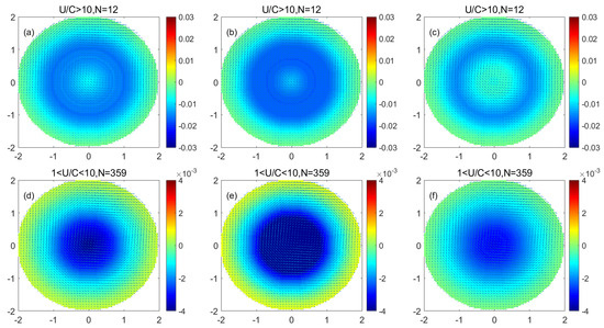
Figure 8.
(a–c) are the monopole distribution of microplankton, nanophytoplankton, and picophytoplankton in a high nonlinear anticyclonic eddy, respectively; (d–f) are the monopole distribution of microplankton, nanophytoplankton, and picophytoplankton in a low nonlinear anticyclonic eddy, respectively. (Unit: mg/m3).
Figure 9 shows that in the monopole decomposition of the anticyclonic eddy, both PP and POC in the center of the eddy decrease, and the reduction in PP and POC in the eddy gradually decreases with the distance from the center of the eddy. PP and POC concentrations increased at the periphery of the eddy. The higher value of PP/Chl in the anticyclonic eddy monopole center indicates that the carbon sequestration efficiency of phytoplankton unit chlorophyll in the anticyclonic center of the eddy is higher. The value of PP/POC in the anticyclonic eddy monopole center is lower, indicating that phytoplankton in anticyclonic eddies are less efficient at generating new productivity. Comparing the physiological status of the high nonlinear anticyclonic eddy and the low nonlinear anticyclonic eddy, it can be found that the reduction in PP, POC, and PP/POC in the high nonlinear anticyclonic eddy is more significant than that in the low nonlinear anticyclonic. In the reduction of PP, POC, and PP/POC in the nonlinear anticyclonic eddy, the PP/Chl of the high nonlinear eddy is larger than the PP/Chl of the low nonlinear eddy. This shows that the vertical effects of high nonlinear anticyclonic eddies have a more significant effect on the physiological status of the eddy than the vertical effect of low nonlinear anticyclonic eddies.
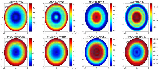
Figure 9.
(a–d) are the monopole distribution of the PP variation, POC variation, PP/Chl, and PP/POC in the high nonlinear anticyclonic eddy, respectively; (e–h) are the monopole distribution of the PP variation, POC variation, PP/Chl, and PP/POC in the low nonlinear anticyclonic eddy, respectively. (Unit: mg/m3).
Figure 10 shows that in the low nonlinear mode-water eddy, microplankton and nanophytoplankton at the center of the eddy increase while picophytoplankton decrease. Microplankton decreased at the periphery of the eddy, while nanophytoplankton and picophytoplankton increased at the periphery of the eddy. The increase in phytoplankton in the center of the eddy saw more nanophytoplankton than microplankton, and the increase in nanoplankton was similar to the increase in picoplankton at the periphery of the eddy. In contrast, the variation in microplankton at the periphery is more significant than that in nanoplankton and picoplankton.
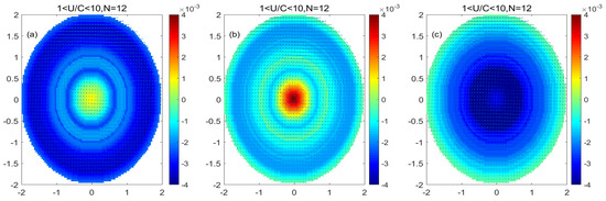
Figure 10.
(a–c) are the monopole distribution of microplankton, nanophytoplankton, and picophytoplankton in low nonlinear mode-water eddy, respectively. (Unit: mg/m3).
Figure 11 shows that in the monopole decomposition of the mode-water eddy, both PP and POC increase in the central eddy of the low nonlinear mode-water eddy, indicating that the increase in eddy phytoplankton in the low nonlinear mode-water eddy causes the eddy internal primary productivity to increase and generates more POC. The value of PP/Chl is lower in the center of the low nonlinear mode-water eddy, indicating that the carbon sequestration efficiency of phytoplankton unit chlorophyll is low in the center of the low nonlinear mode-water eddy. A higher value indicates that the efficiency of phytoplankton in the low nonlinear mode-water eddy in generating new productivity is improved. Comparing the physiological status of low nonlinear anticyclonic eddies and low nonlinear mode-water eddies, the variations in PP and POC in low nonlinear anticyclonic eddies are opposite to those in low nonlinear mode-water eddies. The PP/Chl of the mode-water eddy is smaller than the PP/Chl of the low nonlinear anticyclonic eddy, indicating that the unit chlorophyll carbon fixation efficiency of phytoplankton in the low nonlinear mode-water eddy is smaller than that of the phytoplankton in the low nonlinear anticyclonic eddy.
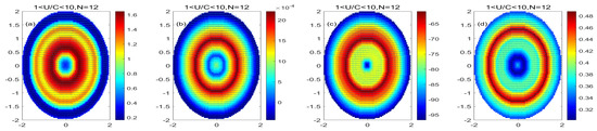
Figure 11.
(a–d) are the monopole distribution of PP variation, POC variation, PP/Chl, and PP/POC in the low nonlinear mode-water eddy, respectively; (Unit: mg/m3).
3.4. 3-Dimensional Vertical Transport Based on HYCOM
The physical properties of the eddy are analyzed from the vertical three-dimensional structure of the temperature inside the mesoscale eddy. Figure 12a shows a negative temperature anomaly (TA) in the mode-water eddy. At 0–75 m, there is a low temperature in the center of the eddy, indicating that the mode-water eddy’s seasonal isothermal uplift indicates that deep cold water enters the surface. However, below 75 m the center of the mode-water eddy has a positive TA, and the temperature at the center of the eddy is higher than the temperature at the periphery of the eddy. The positive TA in the center of mode-water eddy can reach up to 0.5 °C, indicating that the subsurface isotherm of the mode-water eddy sinks. As the depth increases, the positive TA in the eddy gradually weakens. From the three-dimensional temperature structure of the mode-water eddy, the mode-water eddy presents a lens-shaped isocline structure. The positive TA produced by the low nonlinear mode-water eddy in the subsurface is weaker than that produced by the anticyclonic eddy in the subsurface. The surface of the low nonlinear mode-water eddy has negative TA due to the upward surge of cold water, which is entirely different from the positive TA on the surface of the anticyclonic eddy. Compared with the low nonlinear anticyclonic eddy, the positive TA in the low nonlinear mode-water eddy is lower than that in the low nonlinear anticyclonic eddy in the subsurface.
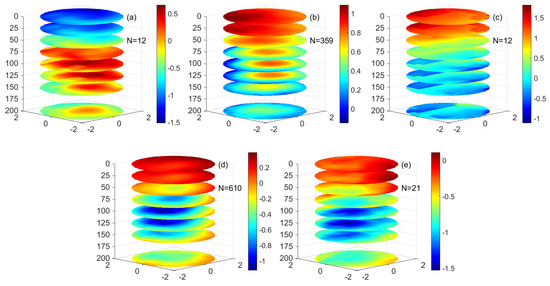
Figure 12.
The three−dimensional structure of temperature anomalies in a different eddy. (a–e) are (a) mode-water eddies, (b) low nonlinear anticyclonic eddies, (c) high nonlinear anticyclonic eddies, (d) low nonlinear cyclonic eddies, and (e) high nonlinear cyclonic eddies. (Unit: °C).
Figure 12b,c shows a positive TA in the center of the anticyclonic eddy. In the anticyclonic eddy, the positive TA at the eddy’s center gradually weakens with increased depth. In the surface layer of the anticyclonic eddy, the positive TA of the eddy exists in the northwest direction of the low nonlinear anticyclonic eddy’s center and a strong positive TA appears inside and outside the strong nonlinearity anticyclonic eddy. From 50 m, the positive TA is in the center of the eddy. Moreover, it continues to weaken from the center of the eddy to the periphery. The positive TA signals increase gradually at 50 m, reaches a peak at 100–125 m, and then gradually weakens. This shows that in the anticyclonic eddy, the temperature structure in the center of the eddy is regulated by the eddy itself, while the temperature structure distribution on the surface of the eddy is not only affected by the eddy itself but also may be affected by the heat of the ocean and atmosphere exchange, ocean surface monsoon, and other factors. A negative TA is also found at the periphery of the low nonlinear anticyclonic eddy from 50–200 m. This may be due to the upwelling caused by the presence of ageostrophic secondary circulation at the periphery of the low nonlinear eddy, which brings deep cold seawater to the euphotic layer. From the perspective of the three-dimensional structure of the eddy, the main isothermal and the seasonal isothermal in the low nonlinear anticyclonic eddy show a downwelling in the anticyclonic eddy, which is similar to the temperature structure inside the anticyclonic eddy in the previous study. There is a cold-water signal at the periphery of the eddy subsurface in the anticyclonic eddy, which may be related to the upwelling of the deep-water body caused by the sub-mesoscale motion of the eddy. The structure of TA at the periphery of the anticyclonic eddy is similar to the chlorophyll ring structure of the anticyclonic eddy in some sea areas, which may be regulated by sub-mesoscale dynamics. Compared with the low nonlinear anticyclonic eddy and the high nonlinear anticyclonic eddy, the temperature structure in the eddy is similar, but there is higher positive TA in the center of the high nonlinear anticyclonic eddy and lower negative temperature anomaly in the periphery of anticyclonic eddy.
Figure 12d,e shows that in the cyclonic eddy there is a negative TA in the eddy’s center. In the surface layer of the low nonlinear cyclonic eddy from 0 m to 25 m, there is a slight positive TA in the eddy, while in the surface layer of the high nonlinear cyclonic eddy there is negative TA in the center of the eddy. Starting from 50 m, the negative TA of the cyclonic eddy center is in the center of the eddy and gradually weakens from the center of the eddy to the outside; the reduction in temperature starts to increase gradually at 50 m, reaches a peak at 100–125 m, and then gradually weakens. This shows that in the cyclonic eddy, the temperature structure in the eddy center is regulated by the eddy-pumping effect, while the temperature structure distribution on the surface of the eddy is not only affected by the eddy itself but also may be affected by the ocean. It is influenced by atmospheric heat exchange and ocean surface monsoons. From the perspective of the three-dimensional structure of the eddy, the main and seasonal isotherms in the cyclonic eddy show an upward trend. Compared with the low nonlinear cyclonic eddy and the high nonlinear cyclonic eddy, the temperature structure in the eddy is similar, but there is lower negative TA in the center of the high nonlinear cyclonic eddy. The temperature difference between high nonlinear eddy and low nonlinear eddy may be caused by the difference of nonlinearity between eddies.
Figure 13a shows that the salinity anomaly (SA) in the eddy is less than 0 in the region of 0–75 m in the low nonlinear mode-water eddy. As the depth increases, the SA in the eddy gradually decreases. The negative SA increases after 75 m, and the intensity of the negative SA gradually decreases in the 75–200 m eddy. The SA produced by the low nonlinear mode-water eddy in the subsurface is more robust than that produced by the anticyclonic eddy in the subsurface.
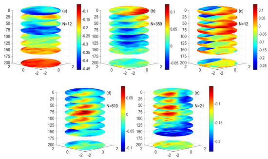
Figure 13.
The three−dimensional structure of salinity anomalies of the different eddies. (a–e) are (a) mode-water eddies, (b) low nonlinear anticyclonic eddies, (c) high nonlinear anticyclonic eddies, (d) low nonlinear cyclonic eddies, and (e) high nonlinear cyclonic eddies. (Unit: PSU).
Figure 13b,c shows a negative SA in the center of the anticyclonic eddy. At 0–50 m of the anticyclonic eddy, the negative SA of the eddy exists in the northwest direction of the eddy’s center. Starting from 50 m, the negative SA is in the center of the anticyclonic eddy. It continues to weaken from the center of the eddy to the periphery. The negative SA signal increases gradually at 50 m, reaching a peak at 100–125 m, and then gradually weakens at 125–200 m. This shows that in the nonlinear anticyclonic eddy, the salinity structure at the center of the eddy is regulated by the eddy itself. There is a positive SA signal at the periphery of the eddy subsurface layer of the anticyclonic eddy, which may be related to the upwelling of the deep-water body caused by the sub-mesoscale motion of the eddy. The structure of SA at the periphery of the eddy is similar to the chlorophyll ring structure of the anticyclonic eddy in some sea areas, which may be regulated by sub-mesoscale dynamics. Compared with the low nonlinear anticyclonic eddy and the high nonlinear anticyclonic eddy, the salinity structure in the eddy is similar, but there is lower negative SA in the center of the high nonlinear anticyclonic eddy.
Figure 13d,e shows that in the low nonlinear cyclonic eddy, there is a positive SA in the center of the eddy, and the strength of the positive SA continues to weaken from the center of the eddy to the outside; the positive SA of the eddy gradually increases with depth, reaches a peak at 100 m, and gradually weakens at the center of the eddy from 100 m to 200 m. This shows that in the nonlinear cyclonic eddy, the salinity structure in the eddy center is regulated by the eddy-pumping effect. From the perspective of the three-dimensional structure of the eddy, the main and seasonal isolines in the low nonlinear cyclonic eddy show an upward trend. Compared with the low nonlinear cyclonic eddy and the high nonlinear cyclonic eddy, the salinity structure in the eddy is similar, but there is higher positive SA in the center of the high nonlinear cyclonic eddy. The salinity difference between high nonlinear eddy and low nonlinear eddy may be caused by the difference of nonlinearity between eddies.
Figure 14a shows the anomalous distribution of the quasi-geostrophic vertical velocity in the low nonlinear mode-water eddy. From 0 m to 50 m, the upward vertical velocity anomaly in the eddy center gradually decreases with depth. From 50 m to 125 m, the downward vertical velocity anomaly in the eddy center is continuously enhanced with increasing depth, and from 125 m to 150 m, the vertical downward speed is continually reduced with increasing depth. This shows that in the mode-water eddy, the seasonal pycnocline of the eddy is uplifted, and the main pycnocline in the subsurface of the eddy is compressed due to the vertical action in the eddy.
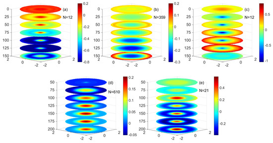
Figure 14.
The three−dimensional monopole structure of ageostrophic vertical velocity and anomalies of the different eddies. (a–e) are (a) mode−water eddies, (b) low nonlinear anticyclonic eddies, (c) high nonlinear anticyclonic eddies, (d) low nonlinear cyclonic eddies, and (e) high nonlinear cyclonic eddies. (Unit: m/d).
Figure 14b,c shows the anomalous distribution of the quasi-geostrophic vertical velocity of the anticyclonic eddy. As the depth increases from 0 to 125 m, the vertical downward velocity at the center of the low nonlinear anticyclonic eddy gradually increases, while at 0–75 m, the vertical downward velocity at the center of the high nonlinear anticyclonic eddy gradually increases. The vertical downward velocity decreases from 125 m to 150 m in the low nonlinear anticyclonic eddy, while the vertical downward velocity in the center of the high nonlinear anticyclonic eddy slowly decreases from 75 m to 150 m. At the periphery of the eddy, the vertical velocity of the eddy will gradually increase from 0 to 125 m and slowly decrease between 125 and 150 m. This shows that in the anticyclonic eddy, the seasonal pycnocline and the main pycnocline in the subsurface of the eddy is compressed due to the vertical action in the eddy. The distribution of quasi-geostrophic vertical velocity anomalies in low nonlinear anticyclonic eddies and high nonlinear anticyclonic eddies is similar. The vertical velocity anomalies in high nonlinear anticyclonic eddies are greater than those in low nonlinear anticyclonic eddies.
Figure 14d,e shows the anomalous distribution of the quasi-geostrophic vertical velocity of the cyclonic eddy. As the depth increases from 0 m to 150 m, the vertical upward velocity at the eddy’s center gradually increases, and the vertical upward velocity decreases after 150 m to 200 m. At the periphery of the eddy, the vertical velocity of the eddy increases gradually downward from 0 m to 125 m and slowly decreases between 125 m and 250 m. The average vertical upward velocity anomaly at the center of the eddy is much larger than the average vertical upward velocity anomaly at the periphery of the eddy. This shows that in the cyclonic eddy, the seasonal pycnocline of the eddy and the main pycnocline in the subsurface of the eddy are uplifted due to the vertical action in the eddy. The vertical velocity anomaly changes in the high nonlinear cyclonic eddy are similar to those in the low nonlinear cyclonic eddy in structure and more significant than those in the low nonlinear cyclonic eddy.
The uneven distribution of phytoplankton in the eddy may be related to the distribution of eddy kinetic energy in the eddy. Figure 15 shows that the EKE correlates with the region’s phytoplankton content. The distribution of the EKE in the eddy was similar to the distribution of phytoplankton of each particle size in the eddy.
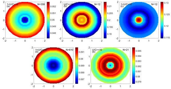
Figure 15.
The monopole distribution of EKE in the eddy. (a) Low nonlinearity anticyclonic eddy. (b) High nonlinearity anticyclonic eddy. (c) Low nonlinearity mode-water eddy. (d) Low nonlinearity cyclonic eddy. (e) High nonlinearity cyclonic eddy. (Unit: m2/s2).
3.5. Temporal Variations in Phytoplankton Size and Physiological Status Extracted from the Eddy-Interior Monopole Results
Figure 16 shows the time series of phytoplankton changes of different particle sizes in the center of the cyclonic and anticyclonic eddies. For different sizes of phytoplankton, the phytoplankton in the center of the cyclonic eddies usually increased, and the phytoplankton in the center of the anticyclonic eddy usually decreased. The changing trends of phytoplankton of different sizes were similar. The phytoplankton change in the eddy’s center was in the order of nanophytoplankton > microplankton > picoplankton. In addition, phytoplankton increased in the eddy’s center before and after winter. For example, in early 2004, early 2008, early 2012, and early 2016, there was a transient increase in phytoplankton in the eddy’s center. The phytoplankton in the eddy’s center usually decreased before and after summer, such as in summer in 2003, summer in 2007, and summer in 2009.
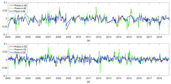
Figure 16.
Anomalous time series of phytoplankton of different sizes in the center of anticyclonic eddies (AEs) (a) and cyclonic eddies (CEs) (b) in the NSCS (unit: mg/m3).
Figure 17 shows the time series of changes in PP and POC in the center of the cyclonic and anticyclonic eddies. The PP and POC in the center of cyclonic eddies usually increased, and the PP and POC in the center of anticyclonic eddies usually decreased. PP and POC generally have similar cyclonic and anticyclonic eddy trends, which is similar to the phytoplankton changes in the eddy. During the time near winter, the PP and the POC in the eddy trend to increase, while the PP and the POC in the eddy trend to decreases near the summer.
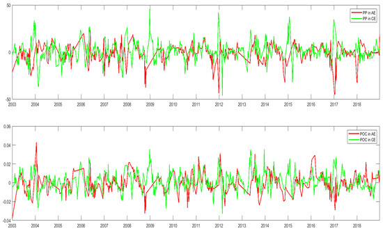
Figure 17.
Anomalous time series of PP and POC in the center of anticyclonic eddies (AEs) and cyclonic eddies (CEs) in the NSCS (unit: mg/m3).
4. Discussion
Figure 5 and Table 1 shows that there are more eddies in winter than in summer in the northern South China Sea, and most mesoscale eddies are observed at the west of Luzon Island, which most of travel westward and tend to move southward along the continental shelf. This study’s distribution of mesoscale eddies is consistent with previous reports [32,38,39,40]. There are few mode-water eddies, which are mainly in summer. The nonlinear eddies gathered near Luzon Island are mainly cyclonic eddies and anticyclonic eddies, most of which appear in winter. While previous studies have shown that nonlinear eddies can capture and transport water masses in the ocean. These eddies may affect the transport of water mass near Luzon Island to the NSCS. The amplitude of the mode-water eddy is more significant than that of the cyclonic eddy and smaller than that of the anticyclonic eddy, indicating that the influence of the mode-water eddy on the eddy pycnocline is between the cyclonic eddy and the anticyclonic eddy. The rotating speed of the mode-water eddy is slightly higher than that of the anti-cyclonic eddy, which is greater than the rotating speed of the cyclonic eddy, indicating that the mode-water eddy is agitated by a high eddy.
The mesoscale eddy-pumping mechanism regulates the increase and decrease in nutrient concentrations within the eddy by regulating the uplift and compress of the seasonal and main isopycnal within the eddy, thereby controlling the increase and decrease in phytoplankton concentration within the eddy. The phytoplankton concentration decreased in the low nonlinear anticyclonic eddy center. The phytoplankton concentration increased in the low nonlinear cyclonic eddy center. Siegel et al. found that a displacement of 4 m of isopycnic occurred per 1 cm of SLA, which was in good agreement with the theoretical value of 5.6 m of vertical isopycnal displacement per cm of dynamic topography [6]. The cyclonic eddy’s low amplitude and the anticyclonic eddy’s high amplitude suggest that this vertical transport of nutrients may be responsible for the chlorophyll changes near the eddy center. In addition, chlorophyll maxima were detected in the western North Pacific and at a depth of approximately 60 m in the South China Sea, with almost 55% of the chlorophyll in the entire water body in the subsurface chlorophyll maxima layer [40]. Therefore, the eddy-induced pumping mechanism cannot be ignored in the chlorophyll displacement in the study area. The higher chlorophyll near the center of the eddy is also reflected in the results of synthetic averaging and often observed as an inverse covariation relationship between SLA and chlorophyll.
Fronts occur at a wide range of scales and are ubiquitous throughout the ocean, curled by persistent wind stress or formed by spatially inhomogeneous surface fluxes of heat and freshwater. Horizontal gradients of buoyancy or fronts help to excite sub-mesoscale dynamics. In the region of the periphery front of the eddy, the isopycnal separates the less dense water from the denser water. When baroclinic instability occurs, an ageostrophic secondary circulation with upwelling and downwelling is generated in the frontal region to restore equilibrium [13]. In the low nonlinear anticyclonic eddy, the periphery of the eddy is the frontal area. There is a strong horizontal gradient with the surrounding water body, so a secondary circulation is generated, which inputs nutrients into the euphotic layer and promotes the growth of phytoplankton. For the high nonlinear anticyclonic eddy, it can be found from the temperature profile that the secondary circulation effect of the high nonlinear anticyclonic eddy is more substantial on the whole due to the enhancement of the horizontal gradient of the eddy periphery.
The concentration of phytoplankton of each size in the cyclonic eddy is generally higher than that in the anticyclonic eddy in the NSCS. Generally, there is a strong correlation between isopycnal displacement and sea level anomalies. The cyclonic eddy triggers upwelling, lifts the isopycnal, and brings the cold and nutrient-rich seawater below the euphotic layer into the euphotic layer. The abundant nutrients stimulate the growth of phytoplankton in the euphotic layer of the cyclonic eddy, and the concentration of chlorophyll on the surface increases; the anticyclonic eddy causes the downwelling to compress the isopycnal, transports the depleted water mass from the euphotic layer to the outside of the euphotic layer, depletes the nutrients in the euphotic layer, inhibits the increase in phytoplankton concentration, and reduces the surface chlorophyll concentration [4,36]. However, in some years, such as 2003, 2007, 2010, and 2016, the chlorophyll variation in the mesoscale eddy has a short time difference from the normal situation. This may indicate that the influence of mesoscale eddies on phytoplankton changes is not only the dynamic mechanism of the eddy itself, but also the influence of interannual changes. The promotional effect of cyclonic eddies on chlorophyll was greater than the inhibitory effect of anticyclonic eddies on chlorophyll. The effect of the mesoscale eddy on surface chlorophyll is not significant in summer, and the effect of mesoscale eddies on surface chlorophyll is significant in winter because the distance between the depth of the mixed layer and the main nutrient layer controls the effect of eddy Ekman suction on chlorophyll. The mesoscale eddy controls the interannual variation in the chlorophyll anomaly within the cyclonic eddy and is closely related to the El Niño Southern Oscillation. Chen et al. studied the cold eddy entering the South China Sea from the Luzon Strait and found that the center of the cyclonic eddy displayed great chlorophyll-a and enhanced nitrate production [21].
Since the NSCS is located in the subtropical water of the earth, from the perspective of biogeochemistry, the influence of the ocean on ecology in the subtropical circulation area is mainly dominated by nutrient limitation. For phytoplankton, the faster-growing cellular phytoplankton are usually microplankton and nanoplankton that cause blooms where nutrients are more readily available. In contrast, slower-growing picophytoplankton are commonly found in subtropical circulations, and for picophytoplankton, Synechococcus can reproduce using nitrate [41,42]. However, Prochlorococcus grows well under ammonium and urea conditions, and grows slowly under nitrate conditions as a nitrogen source. Prochlorococcus accounted for a large proportion of the phytoplankton biomass in the central basin area, but its number was less regulated by nutrients. The nutrient delivery mechanism is weak [13]. In the oligotrophic water of the northern South China Sea, the growth of microplankton and nanophytoplankton is inhibited due to nutrient limitation, and the concentration of phytoplankton in the NSCS is usually small. At the same time, picophytoplankton are weakly affected by nutrient limitation, so they can be abundant in the northern South China Sea. Therefore, the variation in picophytoplankton is dominant in a mesoscale eddy in the NSCS. However, because microplankton and nanophytoplankton are sensitive to nutrient stimulation when nutrients increase in the water, microplankton and nanophytoplankton utilize this part of the nutrients and multiply within a few days, resulting in blooms. When nutrients are depleted in water, the growth of microplankton and nanophytoplankton is again inhibited due to nutrient limitation, and the number of phytoplankton declines rapidly. Therefore, in the long-term series of the different eddies, there are rapid changes in the proportion of microplankton and nanophytoplankton at some time points. Both diatoms and microplankton thrive in cyclonic eddies [21,43]. According to Sathyendranath et al., small-cell phytoplankton predominated in the low chlorophyll-a region, and macro-cell phytoplankton predominated in the high chlorophyll-a region [44]. Phytoplankton size structure covariates with total phytoplankton chlorophyll-a biomass, and in oligotrophic seas, there is a background population of smaller cells that shifts to a larger cell population as nutrients increase the background population [34,45,46,47,48].
It can be known that the mesoscale eddy adjusts the vertical distribution of the eddy’s pycnocline through dynamic mechanics, thereby changing the nutrient environment inside the mesoscale eddy. At the same time, in the oligotrophic sea area, the growth of phytoplankton with larger cells is more sensitive to the stimulation of nutrient concentration. And the northern South China Sea is mainly dominated by nanophytoplankton [49]. Therefore, the decrease in the anticyclonic eddy is nano > micro > pico, and the increase in the cyclonic eddy is nano > micro > pico. In summary, the variation of phytoplankton in the mesoscale eddy is nano > micro > pico.
5. Conclusions
By analyzing the distribution of the different sizes of phytoplankton and related physiological status in different mesoscale eddies, it can be seen that the distribution of the different sizes of phytoplankton and physiological status in the eddies is regulated by the vertical effects of the eddies. The monopole decomposition in the cyclonic eddy indicated that the phytoplankton in the center of the eddy increased due to the vertical action of the eddy, and the corresponding PP and POC contents increased. In addition, the variation in phytoplankton concentration in the cyclonic eddy is nanophytoplankton > microplankton > picophytoplankton—the carbon sequestration efficiency of phytoplankton in cyclonic eddies decreases, resulting in increased new productivity effects. In addition, the variation in phytoplankton concentration in the anticyclonic eddy is nanophytoplankton > microplankton > picophytoplankton—the carbon sequestration efficiency of phytoplankton in the anticyclonic eddy increases, and the new productivity effect decreases. The vertical effects of high nonlinear eddies have more significant effects on the physiological status within the eddy than the vertical effects of low nonlinear eddies. In the low nonlinear mode-water eddy, the phytoplankton in the center of the eddy increases.
From the three-dimensional structure of the temperature anomaly and salinity anomaly in the eddy, it can be seen that the low nonlinear anticyclonic eddy exists in the center of the eddy due to the eddy-pumping effect compressing the seasonal and main isopycnal. The secondary circulation, generated by the large horizontal density gradient difference on both sides of the edge, produces strong upwelling at the periphery of the eddy. The density change in the high nonlinear anticyclonic eddy’s center is more significant than that in the weak nonlinear anticyclonic eddy, and the regulation effect of eddy pumping is more substantial. The secondary circulation effect in the periphery of the eddy increases. In low nonlinear cyclonic eddies, the eddy has seasonal and main isopycnal uplifts by eddy pumping. In the high nonlinear cyclonic eddy, the anomalous changes in temperature and salinity inside the eddy are more significant than those in the low nonlinear cyclonic eddy, indicating that the seasonal and the main isopycnal in the eddy are more significantly uplifted. The eddy-pumping effect is more substantial. The seasonal isopycnal of the mode-water eddy is uplifted, and the main isopycnal is compressed, which means that the mode-water eddy has a lens-shaped structure. This shows that the monopole structure of phytoplankton of each size in the eddy is regulated by the isopycnal changes caused by the vertical action in the eddy.
Author Contributions
Conceptualization, F.L.; Methodology, F.L.; Resources, F.L.; Writing—original draft, J.C.; Writing—review & editing, F.L. All authors have read and agreed to the published version of the manuscript.
Funding
This work was funded by the Strategic Priority Research Program of the Chinese Academy of Sciences (XDA19060502), the Innovation Group Project of Southern Marine Science and Engineering Guangdong Laboratory (Zhuhai) (No. 311020004), the special project for high-resolution earth observation (No. 30-H30C01-9004-19/21), the National Natural Science Foundation of China (grant numbers 41876207 and 41876200), and the Youth Creative Talent Project (Natural Science) of Guangdong (2019TQ05H114).
Institutional Review Board Statement
Not applicable for studies not involving humans or animals.
Informed Consent Statement
Not applicable as this study did not involve human or animal subjects.
Data Availability Statement
The data presented in this study are available on request from the first author or corresponding author.
Acknowledgments
We gratefully acknowledge the dataset obtained from the following sources. The HYCOM data were obtained from https://www.hycom.org/ (accessed on 17 November 2022). The OMEGA3D data and phytoplankton sizes data were obtained from https://marine.copernicus.eu/ (accessed on 17 November 2022). The SLA data were obtained from https://www.aviso.altimetry.fr/ (accessed on 17 November 2022). The POC and Chl data were obtained from https://hermes.acri.fr/ (accessed on 17 November 2022). The cruise data were obtained from https://seabass.gsfc.nasa.gov/ (accessed on 17 November 2022).
Conflicts of Interest
The authors declare no conflict of interest.
References
- McGillicuddy, D.J.; Anderson, L.A.; Bates, N.R.; Bibby, T.; Buesseler, K.O.; Carlson, C.A.; Davis, C.S.; Ewart, C.; Falkowski, P.G.; Goldthwait, S.A.; et al. Eddy/wind interactions stimulate extraordinary mid-ocean plankton blooms. Science 2007, 316, 1021–1026. [Google Scholar] [CrossRef]
- Mahadevan, A.; Thomas, L.N.; Tandon, A. Comment on “eddy/wind interactions stimulate extraordinary mid-ocean plankton blooms”. Science 2008, 320, 448. [Google Scholar] [CrossRef]
- McGillicuddy, D.J. Mechanisms of Physical-Biological-Biogeochemical Interaction at the Oceanic Mesoscale. Annu. Rev. Mar. Sci. 2016, 8, 125–159. [Google Scholar] [CrossRef]
- Siegel, D.A.; Peterson, P.; McGillicuddy, D.J.; Maritorena, S.; Nelson, N.B. Bio-optical footprints created by mesoscale eddies in the Sargasso Sea. Geophys. Res. Lett. 2011, 38, L13608. [Google Scholar] [CrossRef]
- Martin, A.P.; Pondaven, P. On estimates for the vertical nitrate flux due to eddy pumping. J. Geophys. Res.-Oceans 2003, 108, 3359. [Google Scholar] [CrossRef]
- Siegel, D.A.; McGillicuddy, D.J.; Fields, E.A. Mesoscale eddies, satellite altimetry, and new production in the Sargasso Sea. J. Geophys. Res.-Oceans 1999, 104, 13359–13379. [Google Scholar] [CrossRef]
- Gaube, P.; Chelton, D.B.; Samelson, R.M.; Schlax, M.G.; O’Neill, L.W. Satellite Observations of Mesoscale Eddy-Induced Ekman Pumping. J. Phys. Oceanogr. 2015, 45, 104–132. [Google Scholar] [CrossRef]
- Martin, A.P.; Richards, K.J.; Law, C.S.; Liddicoat, M. Horizontal dispersion within an anticyclonic mesoscale eddy. Deep-Sea Res. Part II 2001, 48, 739–755. [Google Scholar] [CrossRef]
- Eden, C.; Dietze, H. Effects of mesoscale eddy/wind interactions on biological new production and eddy kinetic energy. J. Geophys. Res.-Oceans 2009, 114, C05023. [Google Scholar] [CrossRef]
- Kahru, M.; Fiedler, P.C.; Gille, S.T.; Manzano, M.; Mitchell, B.G. Sea level anomalies control phytoplankton biomass in the Costa Rica Dome area. Geophys. Res. Lett. 2007, 34, L22601. [Google Scholar] [CrossRef]
- Kahru, M.; Mitchell, B.G.; Gille, S.T.; Hewes, C.D.; Holm-Hansen, O. Eddies enhance biological production in the Weddell-Scotia confluence of the southern ocean. Geophys. Res. Lett. 2007, 34, L14603. [Google Scholar] [CrossRef]
- Liu, F.F.; Tang, S.L.; Huang, R.X.; Yin, K.D. The asymmetric distribution of phytoplankton in anticyclonic eddies in the western South China Sea. Deep-Sea Res. Part I 2017, 120, 29–38. [Google Scholar] [CrossRef]
- Mahadevan, A. The Impact of Submesoscale Physics on Primary Productivity of Plankton. Annu. Rev. Mar. Sci. 2016, 8, 161–184. [Google Scholar] [CrossRef]
- Mizobata, K.; Saitoh, S.I.; Shiomoto, A.; Miyamura, T.; Shiga, N.; Imai, K.; Toratani, M.; Kajiwara, Y.; Sasaoka, K. Bering Sea cyclonic and anticyclonic eddies observed during summer 2000 and 2001. Prog. Oceanogr. 2002, 55, 65–75. [Google Scholar] [CrossRef]
- Liu, F.F.; Tang, S.L.; Chen, C.Q. Impact of nonlinear mesoscale eddy on phytoplankton distribution in the northern South China Sea. J. Mar. Syst. 2013, 123, 33–40. [Google Scholar] [CrossRef]
- Ning, X.; Chai, F.; Xue, H.; Cai, Y.; Liu, C.; Shi, J. Physical-biological oceanographic coupling influencing phytoplankton and primary production in the South China Sea. J. Geophys. Res.-Oceans 2004, 109, C10005. [Google Scholar] [CrossRef]
- Xiu, P.; Chai, F.; Shi, L.; Xue, H.J.; Chao, Y. A census of eddy activities in the South China Sea during 1993–2007. J. Geophys. Res.-Oceans 2010, 115, C03012. [Google Scholar] [CrossRef]
- Li, Q.Y.; Sun, L.; Liu, S.S.; Xian, T.; Yan, Y.F. A new mononuclear eddy identification method with simple splitting strategies. Remote Sens. Lett. 2014, 5, 65–72. [Google Scholar] [CrossRef]
- Lin, I.I.; Lien, C.C.; Wu, C.R.; Wong, G.T.F.; Huang, C.W.; Chiang, T.L. Enhanced primary production in the oligotrophic South China Sea by eddy injection in spring. Geophys. Res. Lett. 2010, 37, L16602. [Google Scholar] [CrossRef]
- Treguer, P.; Bowler, C.; Moriceau, B.; Dutkiewicz, S.; Gehlen, M.; Aumont, O.; Bittner, L.; Dugdale, R.; Finkel, Z.; Iudicone, D.; et al. Influence of diatom diversity on the ocean biological carbon pump. Nat. Geosci. 2018, 11, 27–37. [Google Scholar] [CrossRef]
- Chen, Y.L.L.; Chen, H.Y.; Lin, I.I.; Lee, M.A.; Chang, J. Effects of cold eddy on Phytoplankton production and assemblages in Luzon Strait bordering the South China Sea. J. Oceanogr. 2007, 63, 671–683. [Google Scholar] [CrossRef]
- Ellwood, M.J.; Strzepek, R.F.; Strutton, P.G.; Trull, T.W.; Fourquez, M.; Boyd, P.W. Distinct iron cycling in a Southern Ocean eddy. Nat. Commun. 2020, 11, 825. [Google Scholar] [CrossRef]
- Frenger, I.; Munnich, M.; Gruber, N.; Knutti, R. Southern Ocean eddy phenomenology. J. Geophys. Res.-Oceans 2015, 120, 7413–7449. [Google Scholar] [CrossRef]
- McGillicuddy, D.J., Jr.; Robinson, A.R.; Siegel, D.A.; Jannasch, H.W.; Johnson, R.; Dickey, T.D.; McNeil, J.; Michaels, A.F.; Knap, A.H. Influence of mesoscale eddies on new production in the Sargasso Sea. Nature 1998, 394, 263–266. [Google Scholar] [CrossRef]
- Barcelo-Llull, B.; Mason, E.; Capet, A.; Pascual, A. Impact of vertical and horizontal advection on nutrient distribution in the southeast Pacific. Ocean Sci. 2016, 12, 1003–1011. [Google Scholar] [CrossRef]
- Xi, H.; Losa, S.N.; Mangin, A.; Garnesson, P.; Bretagnon, M.; Demaria, J.; Soppa, M.A.; D’Andon, O.H.F.; Bracher, A. Global Chlorophyll a Concentrations of Phytoplankton Functional Types With Detailed Uncertainty Assessment Using Multisensor Ocean Color and Sea Surface Temperature Satellite Products. J. Geophys. Res.-Oceans 2021, 126, e2020JC017127. [Google Scholar] [CrossRef]
- Maritorena, S.; d’Andon, O.H.F.; Mangin, A.; Siegel, D.A. Merged satellite ocean color data products using a bio-optical model: Characteristics, benefits and issues. Remote Sens. Environ. 2010, 114, 1791–1804. [Google Scholar] [CrossRef]
- Stramski, D.; Reynolds, R.A.; Babin, M.; Kaczmarek, S.; Lewis, M.R.; Rottgers, R.; Sciandra, A.; Stramska, M.; Twardowski, M.S.; Franz, B.A.; et al. Relationships between the surface concentration of particulate organic carbon and optical properties in the eastern South Pacific and eastern Atlantic Oceans. Biogeosciences 2008, 5, 171–201. [Google Scholar] [CrossRef]
- Behrenfeld, M.J.; Falkowski, P.G. A consumer’s guide to phytoplankton primary productivity models. Limnol. Oceanogr. 1997, 42, 1479–1491. [Google Scholar] [CrossRef]
- Yoshie, N.; Suzuki, K.; Kuwata, A.; Nishioka, J.; Saito, H. Temporal and spatial variations in photosynthetic physiology of diatoms during the spring bloom in the western subarctic Pacific. Mar. Ecol. Prog. Ser. 2010, 399, 39–52. [Google Scholar] [CrossRef]
- Bleck, R. An oceanic general circulation model framed in hybrid isopycnic-Cartesian coordinates. Ocean Model. 2002, 4, 55–88. [Google Scholar] [CrossRef]
- Halliwell, G.R. Evaluation of vertical coordinate and vertical mixing algorithms in the HYbrid-Coordinate Ocean Model (HYCOM). Ocean Model. 2004, 7, 285–322. [Google Scholar] [CrossRef]
- Vidussi, F.; Claustre, H.; Manca, B.B.; Luchetta, A.; Marty, J.C. Phytoplankton pigment distribution in relation to upper thermocline circulation in the eastern Mediterranean Sea during winter. J. Geophys. Res.-Oceans 2001, 106, 19939–19956. [Google Scholar] [CrossRef]
- Uitz, J.; Claustre, H.; Morel, A.; Hooker, S.B. Vertical distribution of phytoplankton communities in open ocean: An assessment based on surface chlorophyll. J. Geophys. Res.-Oceans 2006, 111, C08005. [Google Scholar] [CrossRef]
- Gieskes, W.W.C.; Kraay, G.W.; Nontji, A.; Setiapermana, D.; Sutomo. Monsoonal alternation of a mixed and a layered structure in the phytoplankton of the euphotic zone of the banda sea (Indonesia): A mathematical analysis of algal pigment fingerprints. Neth. J. Sea Res. 1988, 22, 123–137. [Google Scholar] [CrossRef]
- Chelton, D.B.; Schlax, M.G.; Samelson, R.M. Global observations of nonlinear mesoscale eddies. Prog. Oceanogr. 2011, 91, 167–216. [Google Scholar] [CrossRef]
- Schutte, F.; Brandt, P.; Karstensen, J. Occurrence and characteristics of mesoscale eddies in the tropical northeastern Atlantic Ocean. Ocean Sci. 2016, 12, 663–685. [Google Scholar] [CrossRef]
- Ho, C.R.; Kuo, N.J.; Zheng, Q.N.; Soong, Y.S. Dynamically active areas in the South China Sea detected from TOPEX/POSEIDON satellite altimeter data. Remote Sens. Environ. 2000, 71, 320–328. [Google Scholar] [CrossRef]
- Wang, D.X.; Xu, H.Z.; Lin, J.; Hu, J.Y. Anticyclonic Eddies in the Northeastern South China Sea during Winter 2003/2004. J. Oceanogr. 2008, 64, 925–935. [Google Scholar] [CrossRef]
- Wang, G.H.; Chen, D.; Su, J.L. Winter eddy genesis in the eastern south china sea due to orographic wind jets. J. Phys. Oceanogr. 2008, 38, 726–732. [Google Scholar] [CrossRef]
- DuRand, M.D.; Olson, R.J.; Chisholm, S.W. Phytoplankton population dynamics at the Bermuda Atlantic Time-series station in the Sargasso Sea. Deep-Sea Res. Part II 2001, 48, 1983–2003. [Google Scholar] [CrossRef]
- Lindell, D.; Post, A.F. Ultraphytoplankton succession is triggered by deep winter mixing in the gulf of Aqaba (Eilat), Red Sea. Limnol. Oceanogr. 1995, 40, 1130–1141. [Google Scholar] [CrossRef]
- Chen, Y.L.L. Comparisons of primary productivity and phytoplankton size structure in the marginal regions of southern East China Sea. Cont. Shelf Res. 2000, 20, 437–458. [Google Scholar] [CrossRef]
- Sathyendranath, S.; Cota, G.; Stuart, V.; Maass, H.; Platt, T. Remote sensing of phytoplankton pigments: A comparison of empirical and theoretical approaches. Int. J. Remote Sens. 2001, 22, 249–273. [Google Scholar] [CrossRef]
- Ciotti, A.M.; Lewis, M.R.; Cullen, J.J. Assessment of the relationships between dominant cell size in natural phytoplankton communities and the spectral shape of the absorption coefficient. Limnol. Oceanogr. 2002, 47, 404–417. [Google Scholar] [CrossRef]
- Kostadinov, T.S.; Siegel, D.A.; Maritorena, S. Retrieval of the particle size distribution from satellite ocean color observations. J. Geophys. Res.-Oceans 2009, 114, C09015. [Google Scholar] [CrossRef]
- Raimbault, P.; Taupier-Letage, I.; Rodier, M. Vertical Size Distribution of Phytoplankton in the Western Mediterranean Sea during Early Summer. Mar. Ecol. Prog. Ser. 1988, 45, 153–158. [Google Scholar] [CrossRef]
- Yentsch, C.S.; Phinney, D.A. A bridge between ocean optics and microbial ecology. Limnol. Oceanogr. 1989, 34, 1694–1705. [Google Scholar] [CrossRef]
- Li, D.; Yang, S.; Wei, Y.; Wang, X.; Mao, Y.; Guo, C.; Sun, J. Response of Size-Fractionated Chlorophyll a to Upwelling and Kuroshio in Northeastern South China Sea. J. Mar. Sci. Eng. 2022, 10, 784. [Google Scholar] [CrossRef]


Disclaimer/Publisher’s Note: The statements, opinions and data contained in all publications are solely those of the individual author(s) and contributor(s) and not of MDPI and/or the editor(s). MDPI and/or the editor(s) disclaim responsibility for any injury to people or property resulting from any ideas, methods, instructions or products referred to in the content. |
© 2022 by the authors. Licensee MDPI, Basel, Switzerland. This article is an open access article distributed under the terms and conditions of the Creative Commons Attribution (CC BY) license (https://creativecommons.org/licenses/by/4.0/).