Multiscale Feature Fusion for the Multistage Denoising of Airborne Single Photon LiDAR
Abstract
:1. Introduction
- (1)
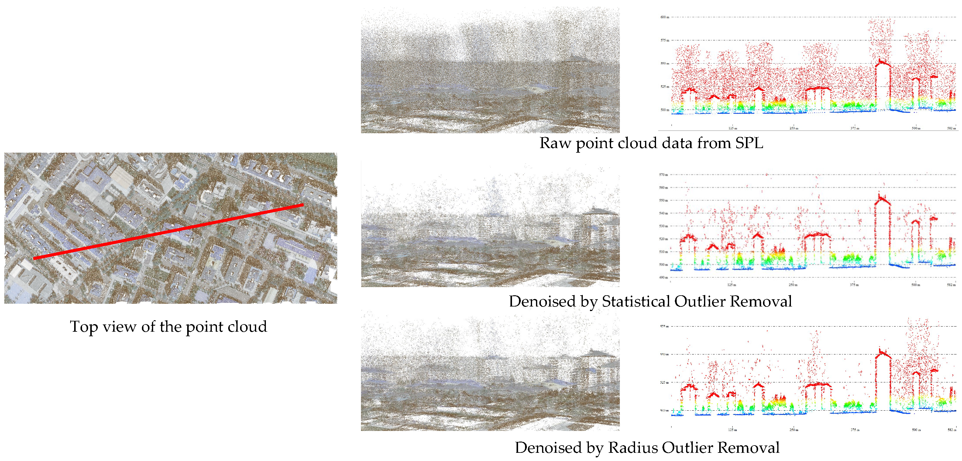
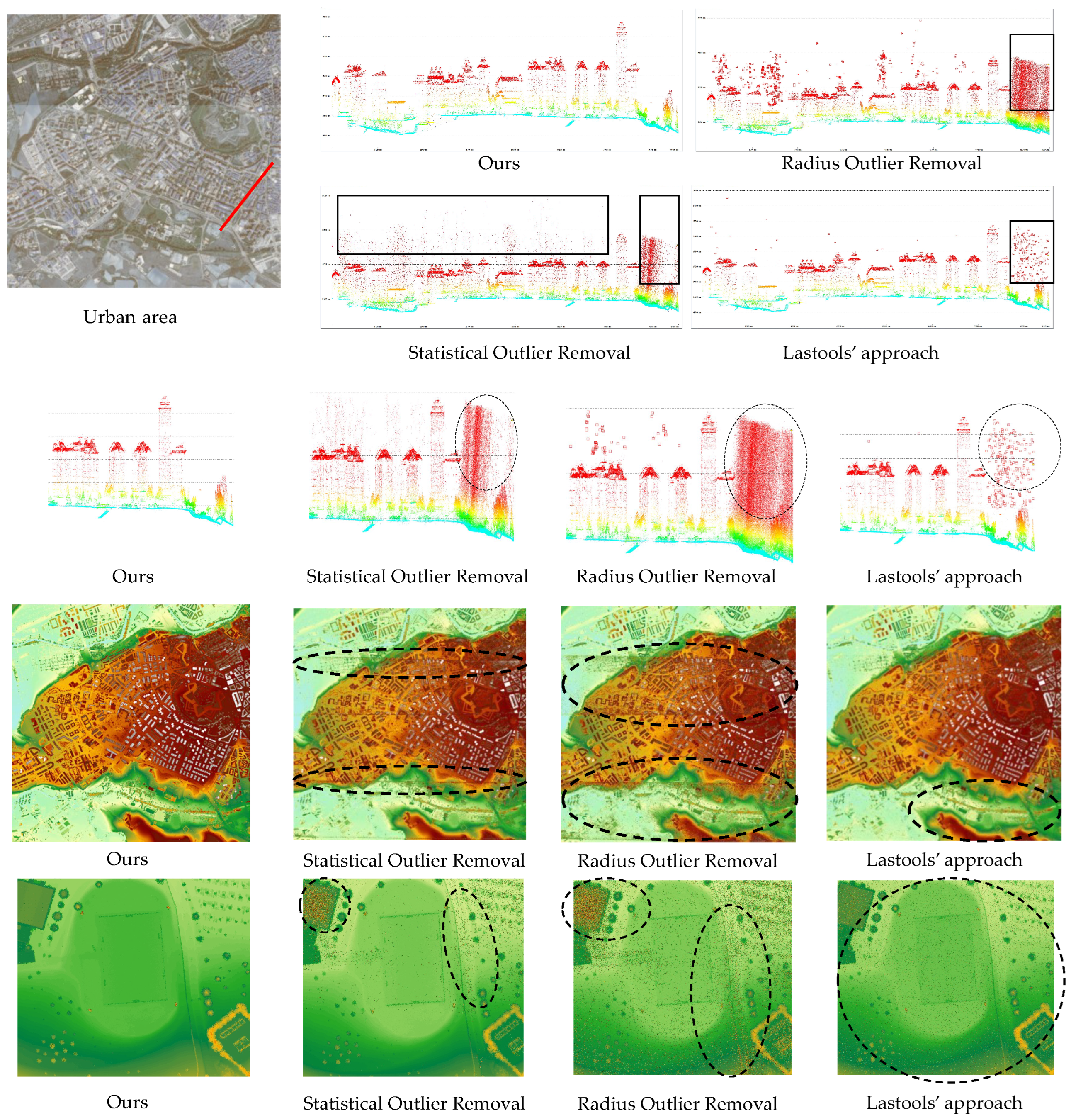
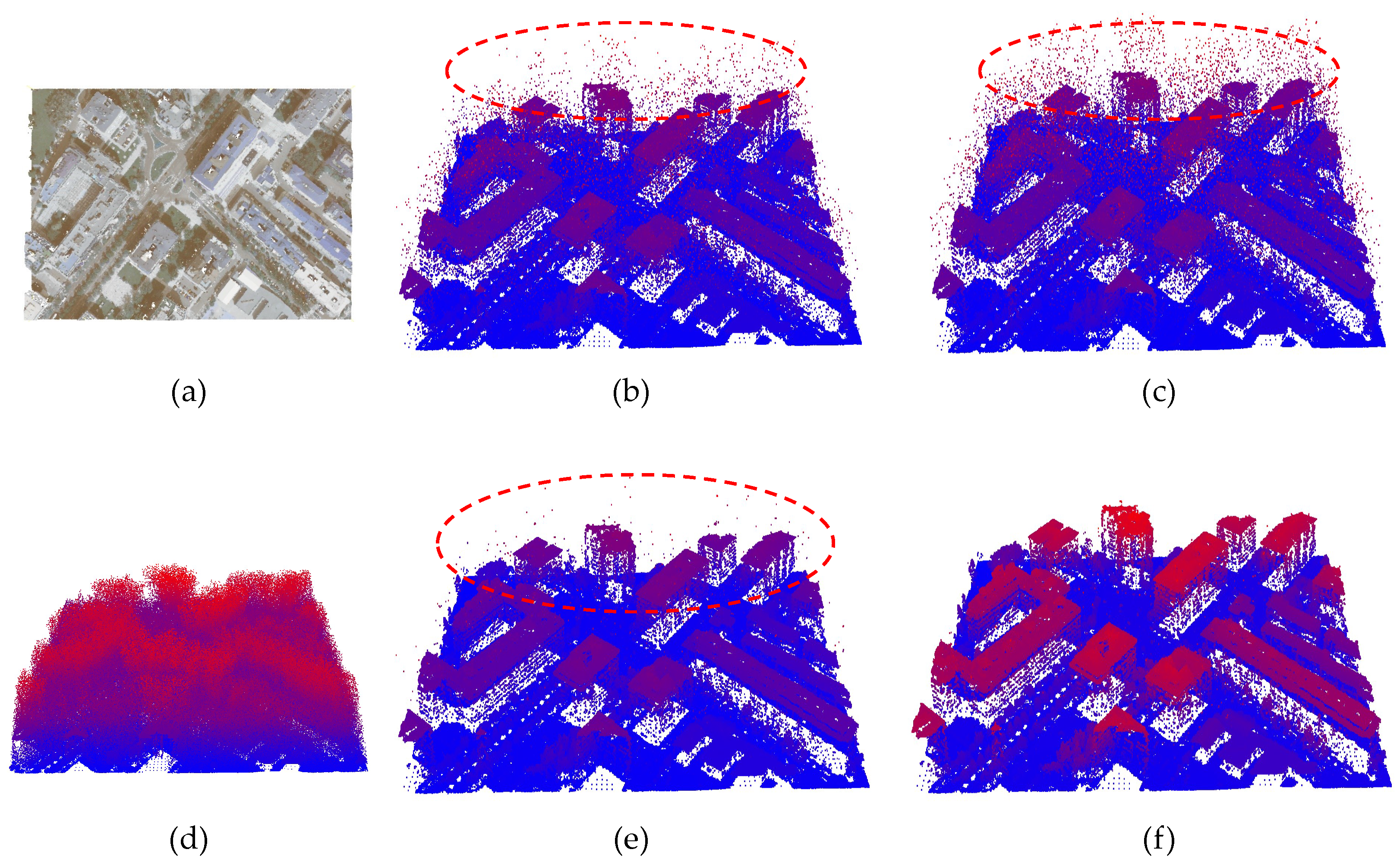
- The sparsity assumption of point cloud noise does not hold: The noise in the LML point clouds is generally sparse, and many existing denoising algorithms have been proposed based on the sparsity assumption. However, the high photon sensitivity of SPL results in numerous noisy points. The noisy point density in the SPL point clouds far exceeds that in the LML point clouds. Therefore, it is hard to remove the noisy points in SPL using existing denoising algorithms (see the second and third rows of Figure 1).
- (2)
- The noisy points cannot be identified with a clear mechanism of generation: The noise in the LML point clouds is primarily due to low outliers generated by the multiple path errors. The low outliers can be removed by morphological opening and closing. In contrast, noisy points in the SPL point clouds are generated for various uncertain reasons, thus, it is difficult to construct a denoising model using a priori knowledge-based method [13].
2. Related Work
2.1. Single-Photon LiDAR
2.2. Point Cloud Denoising
2.3. Point Cloud Features
2.3.1. Neighborhood Definition
2.3.2. Feature Selection
2.3.3. Multiscale Construction
3. Methodology
3.1. Architecture Overview
3.2. Multiscale Hybrid Features of Single-Photon LiDAR
3.2.1. Point-Wise Features
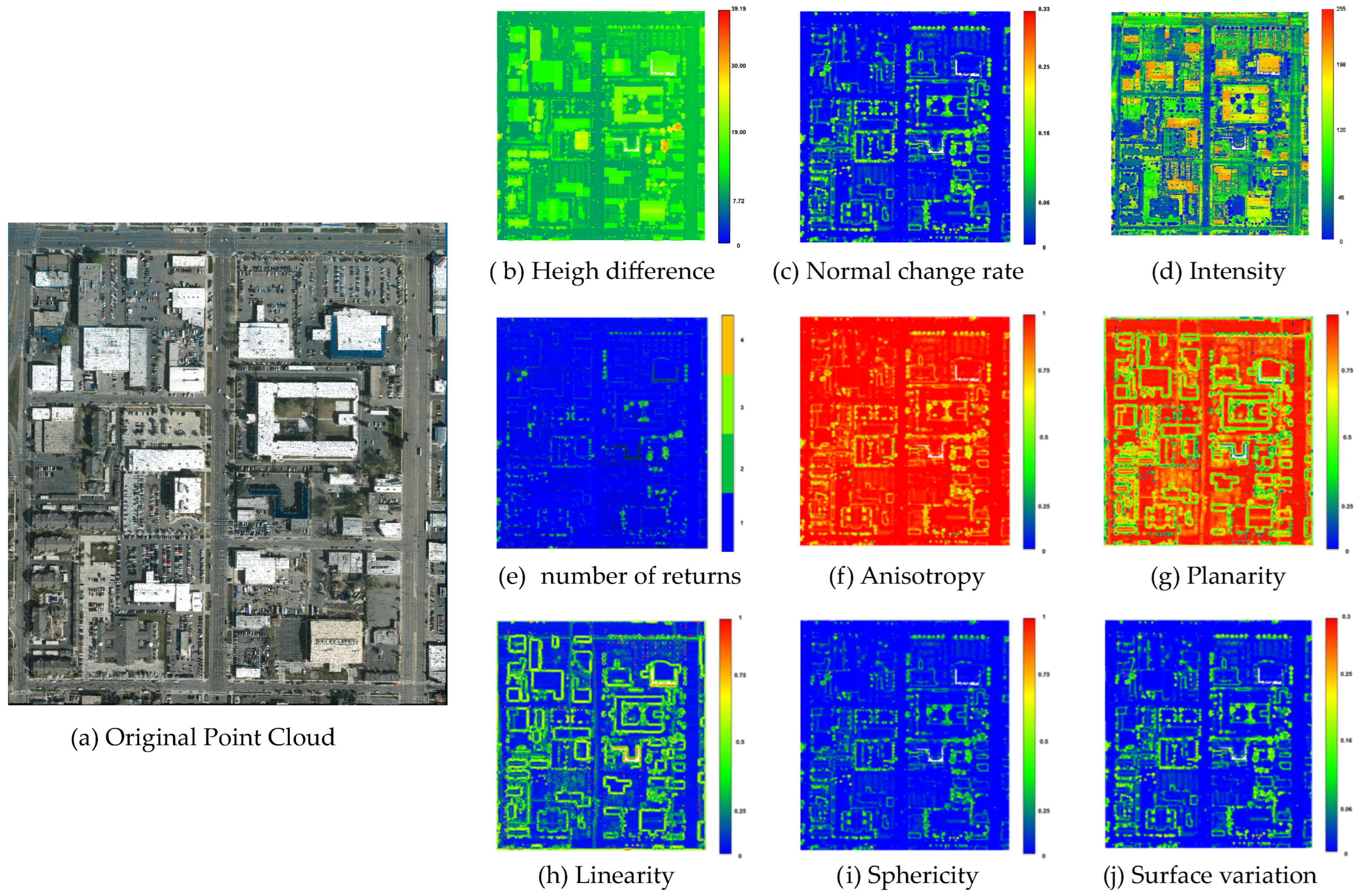
- Intensity-based features: The intensity values reflect the intensity of the reflected signals by the object being measured. The intensity values can distinguish some noisy points from building points, since the intensity of some background noisy points is much lower than that of building points (Figure 3d).
- Echo-based features: N and can describe the echo-based features, where N represents the total number of echoes contained in the current pulse and stands for the normalized number of echoes. Echo-based features can initially extract the vegetation points, since there may be multiple echoes from the same pulse in the vegetation areas (Figure 3e).
3.2.2. Neighborhood-Wise Features
- Height-based features predominantly include height difference (), height standard deviation (), and normal change rate (C). The values of height-based features will be larger in vegetated areas, high noise areas, and building boundaries, where there are more undulations (Figure 3c). We can therefore use height-based features to highlight smooth areas such as ground and building roofs.
- Eigenvalue-based features are widely used for local feature extraction from point clouds, which can effectively portray the distribution of the point cloud in the neighborhood. The eigenvalue-based features are based on the covariance matrix computed within the neighborhood following Equation (1):Here, is a point contained in the neighborhood . The geometric center can be defined by Equation (2):Since the covariance matrix is a symmetric positive-definite matrix, its three eigenvalues , and () exist. Therefore, the eigenvalues can be used to characterize the local neighborhood shapes by calculating the eigenvalue-based features represented by Anisotropy (), Planarity (), Sphericity (), and Linearity (), according to Equations (3)–(6):as shown in Figure 3f–i.
3.2.3. Multiscale Neighborhood Features
3.3. Noise Removal Using Random Forests
4. Experiment
4.1. Datasets
4.2. Evaluation Metrics
4.3. Comparison of Experimental Results
4.3.1. Experiments in the Urban Area
4.3.2. Experiments in the Suburban Area
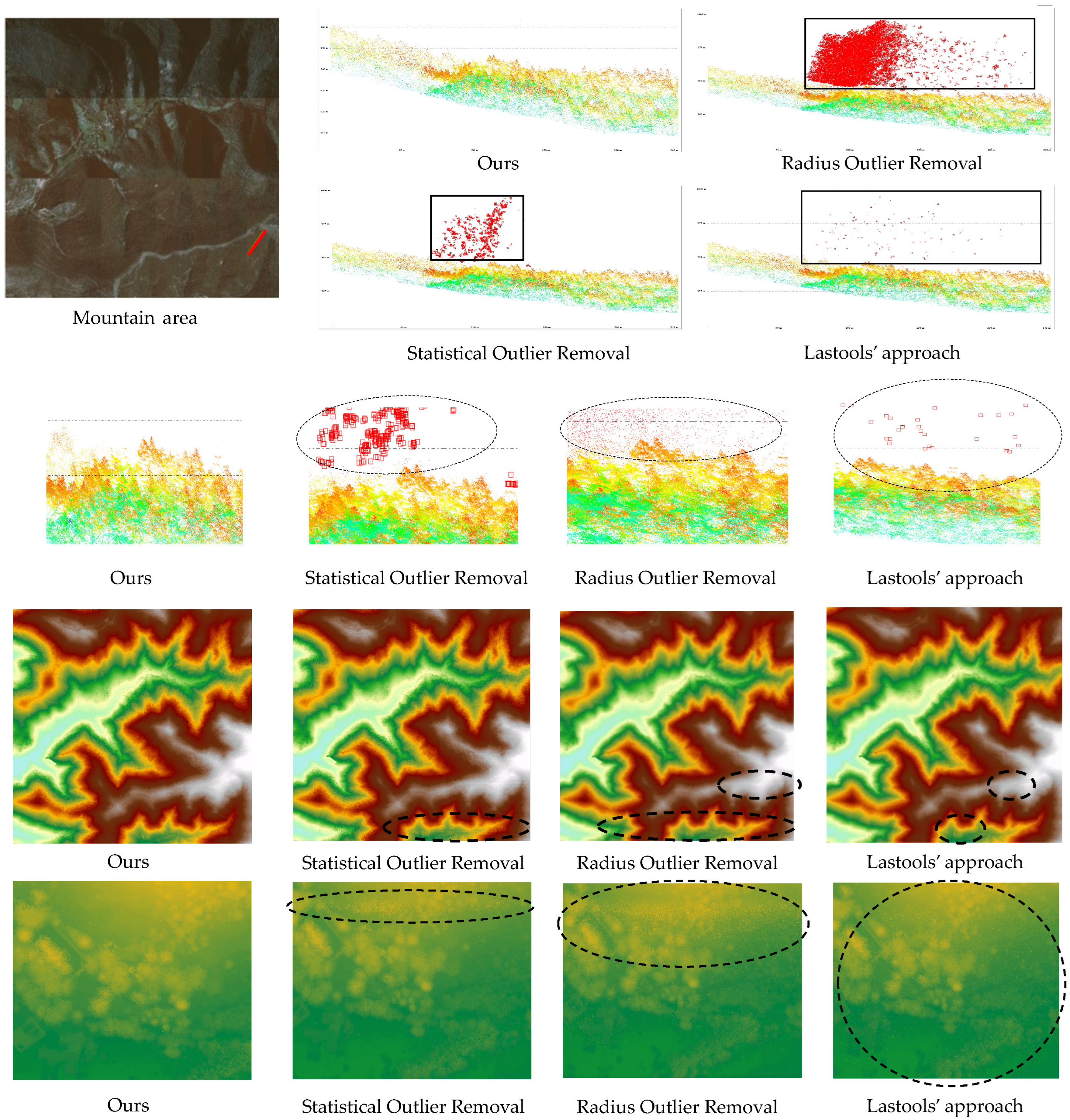
4.3.3. Experiments in the Mountain Area
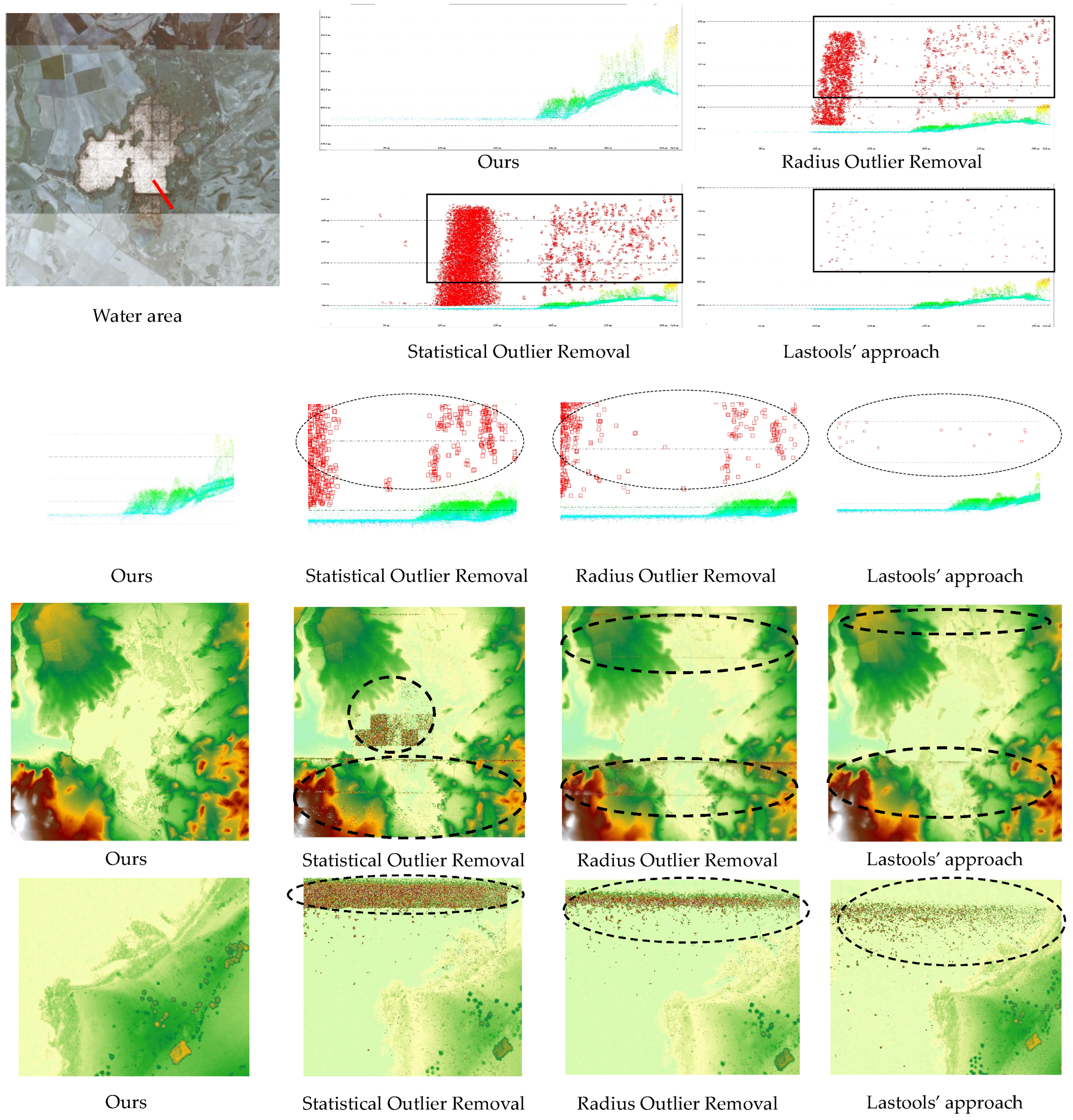
4.3.4. Experiments in the Water Area
4.4. Result Analysis
4.4.1. Analysis of Multiscale Features
4.4.2. Analysis of Multistage Denoising
5. Conclusions
Author Contributions
Funding
Data Availability Statement
Conflicts of Interest
References
- Ye, Z.; Xu, Y.; Huang, R.; Tong, X.; Li, X.; Liu, X.; Luan, K.; Hoegner, L.; Stilla, U. Lasdu: A large-scale aerial lidar dataset for semantic labeling in dense urban areas. ISPRS Int. J. Geo-Inf. 2020, 9, 450. [Google Scholar] [CrossRef]
- Mohtashami, S.; Eliasson, L.; Hansson, L.; Willén, E.; Thierfelder, T.; Nordfjell, T. Evaluating the effect of DEM resolution on performance of cartographic depth-to-water maps, for planning logging operations. Int. J. Appl. Earth Obs. Geoinf. 2022, 108, 102728. [Google Scholar] [CrossRef]
- Jovanović, D.; Milovanov, S.; Ruskovski, I.; Govedarica, M.; Sladić, D.; Radulović, A.; Pajić, V. Building virtual 3D city model for Smart Cities applications: A case study on campus area of the University of Novi Sad. ISPRS Int. J. Geo-Inf. 2020, 9, 476. [Google Scholar] [CrossRef]
- Kukkonen, M.; Maltamo, M.; Korhonen, L.; Packalen, P. Fusion of crown and trunk detections from airborne UAS based laser scanning for small area forest inventories. Int. J. Appl. Earth Obs. Geoinf. 2021, 100, 102327. [Google Scholar] [CrossRef]
- Li, W.; Niu, Z.; Shang, R.; Qin, Y.; Wang, L.; Chen, H. High-resolution mapping of forest canopy height using machine learning by coupling ICESat-2 LiDAR with Sentinel-1, Sentinel-2 and Landsat-8 data. Int. J. Appl. Earth Obs. Geoinf. 2020, 92, 102163. [Google Scholar] [CrossRef]
- Ahola, J.M.; Heikkilä, T.; Raitila, J.; Sipola, T.; Tenhunen, J. Estimation of breast height diameter and trunk curvature with linear and single-photon LiDARs. Ann. For. Sci. 2021, 78, 79. [Google Scholar] [CrossRef]
- Li, Q.; Degnan, J.; Barrett, T.; Shan, J. First Evaluation on Single Photon-Sensitive Lidar Data. Photogramm. Eng. Remote Sens. 2016, 82, 455–463. [Google Scholar] [CrossRef]
- Brown, R.; Hartzell, P.; Glennie, C. Evaluation of SPL100 Single Photon Lidar Data. Remote Sens. 2020, 12, 722. [Google Scholar] [CrossRef] [Green Version]
- Wang, X.; Glennie, C.; Pan, Z. Adaptive noise filtering for single photon Lidar observations. In Proceedings of the 2017 IEEE International Geoscience and Remote Sensing Symposium (IGARSS), Fort Worth, TX, USA, 23–28 July 2017; pp. 3361–3364. [Google Scholar]
- Stoker, J.M.; Abdullah, Q.A.; Nayegandhi, A.; Winehouse, J. Evaluation of Single Photon and Geiger Mode Lidar for the 3D Elevation Program. Remote Sens. 2016, 8, 767. [Google Scholar] [CrossRef] [Green Version]
- White, J.; Woods, M.; Krahn, T.; Papasodoro, C.; Bélanger, D.; Onafrychuk, C.; Sinclair, I. Evaluating the capacity of single photon lidar for terrain characterization under a range of forest conditions. Remote Sens. Environ. 2021, 252, 112169. [Google Scholar] [CrossRef]
- Degnan, J.J. Scanning, Multibeam, Single Photon Lidars for Rapid, Large Scale, High Resolution, Topographic and Bathymetric Mapping. Remote Sens. 2016, 8, 958. [Google Scholar] [CrossRef] [Green Version]
- Mongus, D.; Žalik, B. Parameter-free ground filtering of LiDAR data for automatic DTM generation. ISPRS J. Photogramm. Remote Sens. 2012, 67, 1–12. [Google Scholar] [CrossRef]
- Itzler, M.A.; Entwistle, M.; Wilton, S.; Kudryashov, I.; Kotelnikov, J.; Piccione, B.; Owens, M.; Rangwala, S. Geiger-Mode LiDAR: From Airborne Platforms To Driverless Cars. In Proceedings of the Applied Industrial Optics: Spectroscopy, Imaging and Metrology, San Francisco, CA, USA, 26–29 June 2017; Optical Society of America: Washington, DC, USA, 2017; p. ATu3A.3. [Google Scholar]
- Wu, D.; Zheng, T.; Wang, L.; Chen, X.; Yang, L.; Li, Z.; Wu, G. Multi-beam single-photon LiDAR with hybrid multiplexing in wavelength and time. Opt. Laser Technol. 2022, 145, 107477. [Google Scholar] [CrossRef]
- Abdullah, Q.A. A star is born: The state of new lidar technologies. Photogramm. Eng. Remote Sens. 2016, 82, 307–312. [Google Scholar] [CrossRef]
- Leica. Leica SPL100 Single Photon LiDAR Sensor Data Sheet. Available online: https://leica-geosystems.com/en-us/products/airborne-systems/topographic-lidar-sensors/leica-spl100 (accessed on 17 February 2017).
- Mandlburger, G.; Lehner, H.; Pfeifer, N. A comparison of single photon and full waveform LiDAR. ISPRS Ann. Photogramm. Remote Sens. Spat. Inf. Sci. 2019, 4, 397–404. [Google Scholar] [CrossRef] [Green Version]
- Mandlburger, G.; Jutzi, B. On the Feasibility of Water Surface Mapping with Single Photon LiDAR. ISPRS Int. J. Geo-Inf. 2019, 8, 188. [Google Scholar] [CrossRef] [Green Version]
- Jutzi, B. Less Photons for More LiDAR? A Review from Multi-Photon Detection to Single Photon Detection. In Proceedings of the 56th Photogrammetric Week (PhoWo 2017), Stuttgart, Germany, 11–15 September 2017; p. 6S. [Google Scholar]
- Swatantran, A.; Tang, H.; Barrett, T.; DeCola, P.; Dubayah, R. Rapid, High-Resolution Forest Structure and Terrain Mapping over Large Areas using Single Photon Lidar. Sci. Rep. 2016, 6, 28277. [Google Scholar] [CrossRef] [Green Version]
- Wang, X.; Glennie, C.; Pan, Z. Weak Echo Detection from Single Photon Lidar Data Using a Rigorous Adaptive Ellipsoid Searching Algorithm. Remote Sens. 2018, 10, 1035. [Google Scholar] [CrossRef] [Green Version]
- Vacek, M.; Peca, M.; Michalek, V.; Prochazka, I. Single photon laser altimeter data processing, analysis and experimental validation. Adv. Space Res. 2015, 56, 1307–1318. [Google Scholar] [CrossRef]
- Chen, B.; Pang, Y. A denoising approach for detection of canopy and ground from ICESat-2’s airborne simulator data in Maryland, USA. In AOPC 2015: Advances in Laser Technology and Applications; SPIE: Bellingham, WA, USA, 2015; Volume 9671, p. 96711S. [Google Scholar]
- Zhao, Q.; Gao, X.; Li, J.; Luo, L. Optimization Algorithm for Point Cloud Quality Enhancement Based on Statistical Filtering. J. Sens. 2021, 2021, e7325600. [Google Scholar] [CrossRef]
- Duan, Y.; Yang, C.; Chen, H.; Yan, W.; Li, H. Low-complexity point cloud denoising for LiDAR by PCA-based dimension reduction. Opt. Commun. 2021, 482, 126567. [Google Scholar] [CrossRef]
- Zhang, H.; Zhu, L.; Cai, X.; Dong, L. Noise removal algorithm based on point cloud classification. In Proceedings of the 2022 International Seminar on Computer Science and Engineering Technology (SCSET), Indianapolis, IN, USA, 8–9 January 2022; pp. 93–96. [Google Scholar]
- Balta, H.; Velagic, J.; Bosschaerts, W.; De Cubber, G.; Siciliano, B. Fast Statistical Outlier Removal Based Method for Large 3D Point Clouds of Outdoor Environments. IFAC-PapersOnLine 2018, 51, 348–353. [Google Scholar] [CrossRef]
- Wang, X.; Pan, Z.; Glennie, C. A Novel Noise Filtering Model for Photon-Counting Laser Altimeter Data. IEEE Geosci. Remote Sens. Lett. 2016, 13, 947–951. [Google Scholar] [CrossRef]
- Lin, R.; Hu, H.; Wen, Z.; Yin, L. Research on denoising and segmentation algorithm application of pigs’ point cloud based on DBSCAN and PointNet. In Proceedings of the 2021 IEEE International Workshop on Metrology for Agriculture and Forestry (MetroAgriFor), Trento-Bolzano, Italy, 3–5 November 2021; pp. 42–47. [Google Scholar]
- Zhu, X.; Nie, S.; Wang, C.; Xi, X.; Wang, J.; Li, D.; Zhou, H. A Noise Removal Algorithm Based on OPTICS for Photon-Counting LiDAR Data. IEEE Geosci. Remote Sens. Lett. 2021, 18, 1471–1475. [Google Scholar] [CrossRef]
- Zaman, F.; Wong, Y.P.; Ng, B.Y. Density-Based Denoising of Point Cloud. In Proceedings of the 9th International Conference on Robotic, Vision, Signal, Processing and Power Applications; Springer: Singapore, 2017; pp. 287–295. [Google Scholar]
- Liu, Z.; Xiao, X.; Zhong, S.; Wang, W.; Li, Y.; Zhang, L.; Xie, Z. A feature-preserving framework for point cloud denoising. Comput.-Aided Des. 2020, 127, 102857. [Google Scholar] [CrossRef]
- Digne, J.; de Franchis, C. The Bilateral Filter for Point Clouds. Image Process. On Line 2017, 7, 278–287. [Google Scholar] [CrossRef] [Green Version]
- Han, X.F.; Jin, J.S.; Wang, M.J.; Jiang, W.; Gao, L.; Xiao, L. A review of algorithms for filtering the 3D point cloud. Signal Process. Image Commun. 2017, 57, 103–112. [Google Scholar] [CrossRef]
- Ji, C.; Li, Y.; Fan, J.; Lan, S. A Novel Simplification Method for 3D Geometric Point Cloud Based on the Importance of Point. IEEE Access 2019, 7, 129029–129042. [Google Scholar] [CrossRef]
- Weinmann, M.; Jutzi, B.; Hinz, S.; Mallet, C. Semantic point cloud interpretation based on optimal neighborhoods, relevant features and efficient classifiers. ISPRS J. Photogramm. Remote Sens. 2015, 105, 286–304. [Google Scholar] [CrossRef]
- Wang, Y.; Chen, Q.; Liu, L.; Li, K. A Hierarchical unsupervised method for power line classification from airborne LiDAR data. Int. J. Digit. Earth 2019, 12, 1406–1422. [Google Scholar] [CrossRef]
- Blomley, R.; Weinmann, M. Using multiscale features for the 3D semantic labeling of airborne laser scanning data. ISPRS Ann. Photogramm. Remote Sens. Spat. Inf. Sci. 2017, 4, 43–50. [Google Scholar] [CrossRef] [Green Version]
- Dittrich, A.; Weinmann, M.; Hinz, S. Analytical and numerical investigations on the accuracy and robustness of geometric features extracted from 3D point cloud data. ISPRS J. Photogramm. Remote Sens. 2017, 126, 195–208. [Google Scholar] [CrossRef]
- Singh, S.; Sreevalsan-Nair, J. Adaptive Multiscale Feature Extraction in a Distributed System for Semantic Classification of Airborne LiDAR Point Clouds. IEEE Geosci. Remote Sens. Lett. 2022, 19, 1–5. [Google Scholar] [CrossRef]
- Che, E.; Jung, J.; Olsen, M.J. Object Recognition, Segmentation, and Classification of Mobile Laser Scanning Point Clouds: A State of the Art Review. Sensors 2019, 19, 810. [Google Scholar] [CrossRef] [Green Version]
- Tomková, M.; Lysák, J.; Potůčková, M. Semantic classification of sandstone landscape point cloud based on neighbourhood features. Int. Arch. Photogramm. Remote Sens. Spat. Inf. Sci. 2020, 43, 333–338. [Google Scholar] [CrossRef]
- Gallwey, J.; Eyre, M.; Coggan, J. A machine learning approach for the detection of supporting rock bolts from laser scan data in an underground mine. Tunn. Undergr. Space Technol. 2021, 107, 103656. [Google Scholar] [CrossRef]
- Ni, H.; Lin, X.; Zhang, J. Classification of ALS Point Cloud with Improved Point Cloud Segmentation and Random Forests. Remote Sens. 2017, 9, 288. [Google Scholar] [CrossRef] [Green Version]
- Vetrivel, A.; Gerke, M.; Kerle, N.; Nex, F.; Vosselman, G. Disaster damage detection through synergistic use of deep learning and 3D point cloud features derived from very high resolution oblique aerial images, and multiple-kernel-learning. ISPRS J. Photogramm. Remote Sens. 2018, 140, 45–59. [Google Scholar] [CrossRef]
- Thomas, H.; Goulette, F.; Deschaud, J.E.; Marcotegui, B.; LeGall, Y. Semantic classification of 3D point clouds with multiscale spherical neighborhoods. In Proceedings of the 2018 International Conference on 3D vision (3DV), Verona, Italy, 5–8 September 2018; IEEE: Piscataway, NJ, USA, 2018; pp. 390–398. [Google Scholar]
- Wang, C.; Shu, Q.; Wang, X.; Guo, B.; Liu, P.; Li, Q. A random forest classifier based on pixel comparison features for urban LiDAR data. ISPRS J. Photogramm. Remote Sens. 2019, 148, 75–86. [Google Scholar] [CrossRef]
- Yastikli, N.; Cetin, Z. Classification of LiDAR data with point based classification methods. ISPRS Int. Arch. Photogramm. Remote Sens. Spat. Inf. Sci. 2016, XLI-B3, 441–445. [Google Scholar] [CrossRef]
- Lucas, C.; Bouten, W.; Koma, Z.; Kissling, W.D.; Seijmonsbergen, A.C. Identification of Linear Vegetation Elements in a Rural Landscape Using LiDAR Point Clouds. Remote Sens. 2019, 11, 292. [Google Scholar] [CrossRef] [Green Version]
- Brodu, N.; Lague, D. 3D terrestrial lidar data classification of complex natural scenes using a multiscale dimensionality criterion: Applications in geomorphology. ISPRS J. Photogramm. Remote Sens. 2012, 68, 121–134. [Google Scholar] [CrossRef] [Green Version]
- Dong, W.; Lan, J.; Liang, S.; Yao, W.; Zhan, Z. Selection of LiDAR geometric features with adaptive neighborhood size for urban land cover classification. Int. J. Appl. Earth Obs. Geoinf. 2017, 60, 99–110. [Google Scholar] [CrossRef]
- Demantke, J.; Mallet, C.; David, N.; Vallet, B. Dimensionality based scale selection in 3D LiDAR point clouds. ISPRS Int. Arch. Photogramm. Remote Sens. Spat. Inf. Sci. 2011, 38, W12. [Google Scholar] [CrossRef] [Green Version]
- Huang, R.; Hong, D.; Xu, Y.; Yao, W.; Stilla, U. Multi-Scale Local Context Embedding for LiDAR Point Cloud Classification. IEEE Geosci. Remote Sens. Lett. 2020, 17, 721–725. [Google Scholar] [CrossRef]
- Singh, S.K.; Raval, S.; Banerjee, B. A robust approach to identify roof bolts in 3D point cloud data captured from a mobile laser scanner. Int. J. Min. Sci. Technol. 2021, 31, 303–312. [Google Scholar] [CrossRef]
- Breiman, L. Random Forests. Mach. Learn. 2001, 45, 5–32. [Google Scholar] [CrossRef] [Green Version]
- Blanco, J.L.; Rai, P.K. Nanoflann: A C++ header-only fork of FLANN, a library for Nearest Neighbor (NN) with KD-trees. 2014. Available online: https://github.com/jlblancoc/nanoflann (accessed on 2 May 2014).
- Wright, M.N.; Ziegler, A. Ranger: A Fast Implementation of Random Forests for High Dimensional Data in C++ and R. J. Stat. Softw. 2017, 77, 1–17. [Google Scholar] [CrossRef] [Green Version]
- Mandlburger, G.; Jutzi, B. Feasibility investigation on single photon LiDAR based water surface mapping. ISPRS Ann. Photogramm. Remote Sens. Spat. Inf. Sci. 2018, IV-1, 109–116. [Google Scholar] [CrossRef]
- Government, N. Navarra Dataset. Available online: https://filescartografia.navarra.es (accessed on 19 March 2019).
- Hu, Q.; Yang, B.; Xie, L.; Rosa, S.; Guo, Y.; Wang, Z.; Trigoni, N.; Markham, A. RandLA-Net: Efficient Semantic Segmentation of Large-Scale Point Clouds. In Proceedings of the IEEE/CVF Conference on Computer Vision and Pattern Recognition (CVPR), Seattle, WA, USA, 13–19 June 2020; pp. 11108–11117. [Google Scholar]
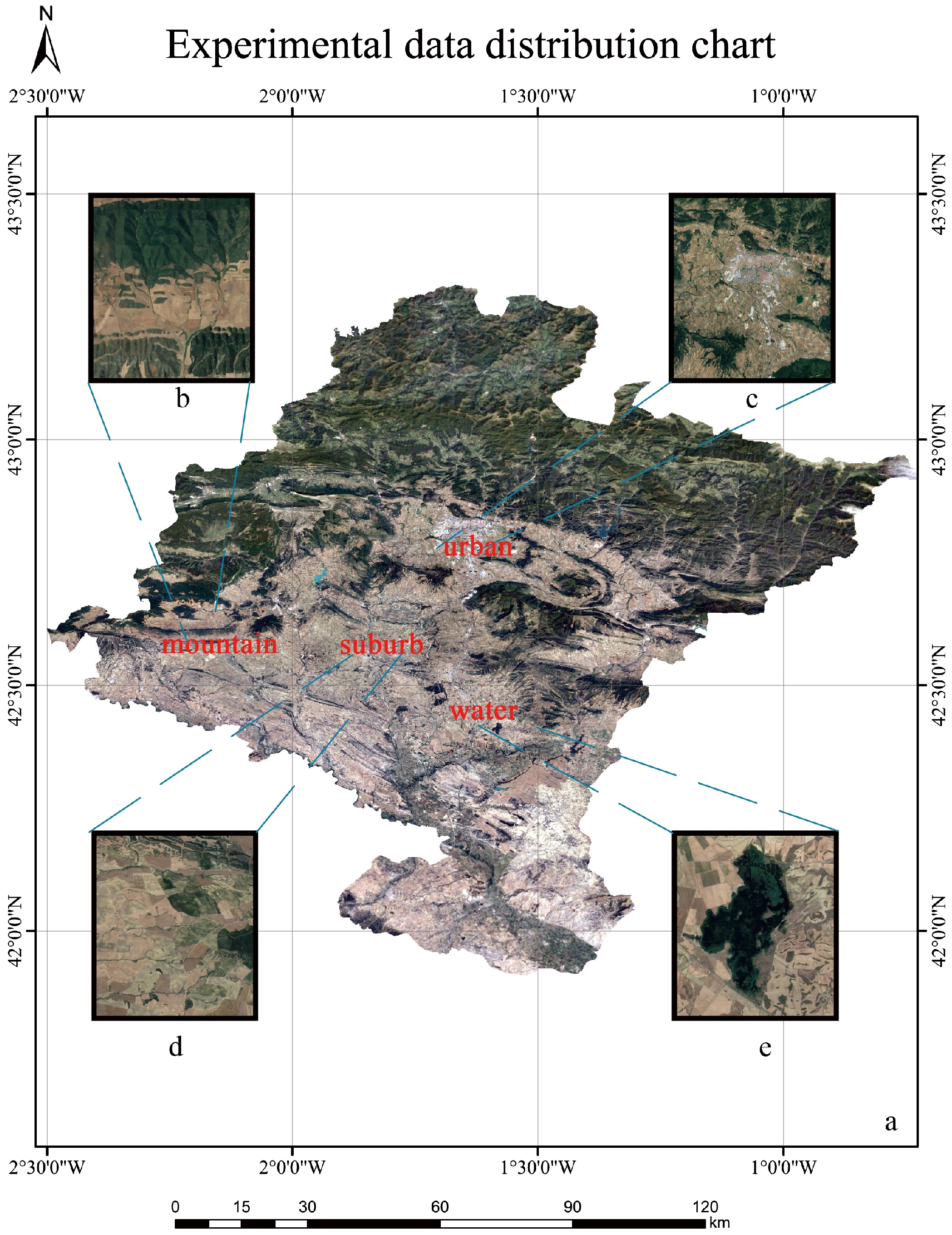


| Dataset Name | Navarra Dataset |
|---|---|
| LiDAR system | SPL100 |
| Point density | 14.5 points/m |
| Flight height | 4200 m (AGL) |
| Field of view (FoV) | 30° |
| Flight speed | 90 m/s |
| Swath width | 2260 m |
| Effective scan rate | 6 MHz |
| Data coverage | The Navarra province of Spain |
| Coordinate system | ETRS89 / UTM zone 30 N (EPSG25830) |
| Methods | Recall (%) | Precision (%) | Accuracy (%) | F1-Score (%) |
|---|---|---|---|---|
| Radius Outlier Removal | 82.63 | 98.51 | 93.71 | 89.87 |
| Statistical Outlier Removal | 65.34 | 99.55 | 88.19 | 78.89 |
| Lastools’ Denoising Workflow | 88.84 | 99.25 | 95.83 | 93.76 |
| RandLA-Net | 93.98 | 94.76 | 94.07 | 94.37 |
| Ours | 96.82 | 98.35 | 98.38 | 97.58 |
| Methods | Recall (%) | Precision (%) | Accuracy (%) | F1-Score (%) |
|---|---|---|---|---|
| Radius Outlier Removal | 94.01 | 99.97 | 98.70 | 96.90 |
| Statistical Outlier Removal | 93.05 | 99.99 | 98.49 | 96.39 |
| Lastools’ Denoising Workflow | 88.52 | 99.98 | 97.22 | 93.91 |
| RandLA-Net | 98.81 | 99.20 | 98.81 | 99.01 |
| Ours | 99.86 | 99.31 | 99.82 | 99.59 |
| Methods | Recall (%) | Precision (%) | Accuracy (%) | F1-Score (%) |
|---|---|---|---|---|
| Radius Outlier Removal | 88.86 | 99.04 | 97.46 | 93.68 |
| Statistical Outlier Removal | 87.90 | 99.44 | 97.33 | 93.32 |
| Lastools’ Denoising Workflow | 87.36 | 99.74 | 96.99 | 93.14 |
| RandLA-Net | 96.48 | 94.26 | 96.48 | 95.35 |
| Ours | 99.47 | 92.22 | 98.11 | 95.70 |
| Methods | Recall (%) | Precision (%) | Accuracy (%) | F1-Score (%) |
|---|---|---|---|---|
| Radius Outlier Removal | 37.58 | 87.11 | 71.57 | 52.51 |
| Statistical Outlier Removal | 31.19 | 98.63 | 71.04 | 47.40 |
| Lastools’ Denoising Workflow | 45.74 | 98.41 | 74.19 | 62.46 |
| Ours | 71.49 | 85.61 | 83.05 | 77.92 |
| Areas | Metrics | Neighborhood (m) | ||||
|---|---|---|---|---|---|---|
| 5 | 10 | 15 | 5, 10 | 5, 10, 15 | ||
| Urban | Accuracy | 96.60 | 97.15 | 97.74 | 98.04 | 98.38 |
| F1-score | 94.97 | 95.72 | 96.61 | 97.08 | 97.58 | |
| Mountain | Accuracy | 94.82 | 95.33 | 95.37 | 96.91 | 98.11 |
| F1-score | 88.86 | 89.81 | 89.98 | 93.16 | 95.70 | |
| Suburban | Accuracy | 98.54 | 98.83 | 99.27 | 99.59 | 99.82 |
| F1-score | 96.70 | 97.28 | 98.31 | 99.06 | 99.59 | |
| Water | Accuracy | 77.35 | 79.66 | 79.44 | 82.65 | 83.05 |
| F1-score | 71.46 | 74.35 | 72.71 | 77.49 | 77.92 | |
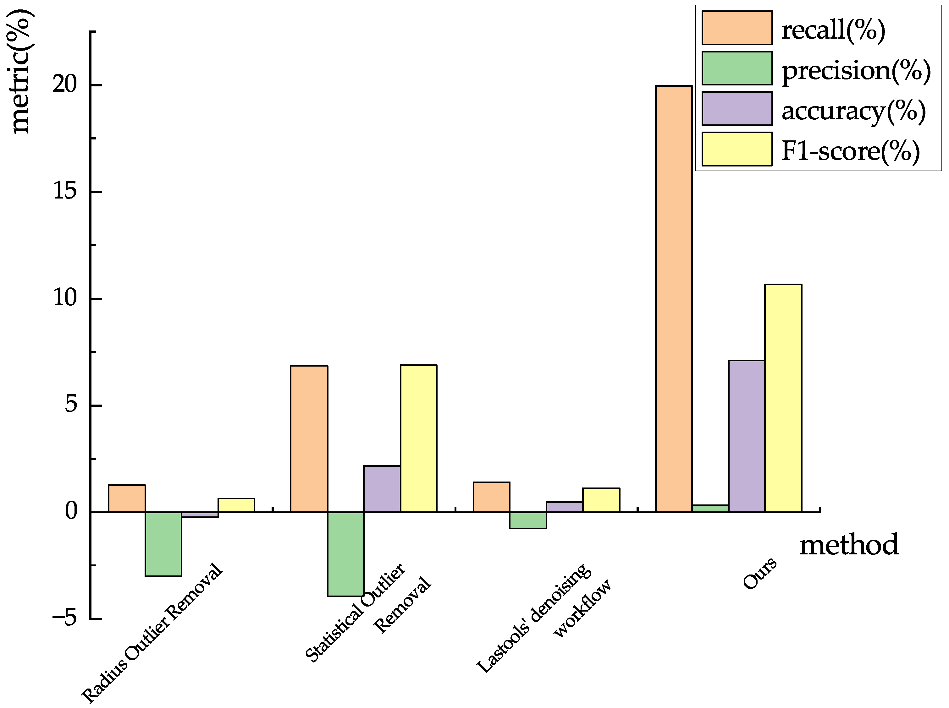
| Methods | Metric | First Denoising | Second Denoising | Improvement |
|---|---|---|---|---|
| Radius Outlier Removal | Recall (%) | 37.58 | 38.85 | 1.27 |
| Precision (%) | 87.11 | 84.12 | −2.99 | |
| Accuracy (%) | 71.57 | 71.35 | −0.22 | |
| F1-score (%) | 52.51 | 53.15 | 0.64 | |
| Statistical Outlier Removal | Recall (%) | 31.19 | 38.05 | 6.86 |
| Precision (%) | 98.63 | 94.70 | −3.93 | |
| Accuracy (%) | 71.04 | 73.20 | 2.16 | |
| F1-score (%) | 47.40 | 54.29 | 6.89 | |
| Lastools’ Denoising Workflow | Recall (%) | 45.74 | 47.14 | 1.40 |
| Precision (%) | 98.41 | 97.64 | −0.77 | |
| Accuracy (%) | 74.19 | 74.66 | 0.47 | |
| F1-score (%) | 62.46 | 63.58 | 1.12 | |
| Ours | Recall (%) | 71.49 | 91.44 | 19.95 |
| Precision (%) | 85.61 | 85.94 | 0.33 | |
| Accuracy (%) | 83.05 | 90.16 | 7.11 | |
| F1-score (%) | 77.92 | 88.60 | 10.68 |
Disclaimer/Publisher’s Note: The statements, opinions and data contained in all publications are solely those of the individual author(s) and contributor(s) and not of MDPI and/or the editor(s). MDPI and/or the editor(s) disclaim responsibility for any injury to people or property resulting from any ideas, methods, instructions or products referred to in the content. |
© 2023 by the authors. Licensee MDPI, Basel, Switzerland. This article is an open access article distributed under the terms and conditions of the Creative Commons Attribution (CC BY) license (https://creativecommons.org/licenses/by/4.0/).
Share and Cite
Si, S.; Hu, H.; Ding, Y.; Yuan, X.; Jiang, Y.; Jin, Y.; Ge, X.; Zhang, Y.; Chen, J.; Guo, X. Multiscale Feature Fusion for the Multistage Denoising of Airborne Single Photon LiDAR. Remote Sens. 2023, 15, 269. https://doi.org/10.3390/rs15010269
Si S, Hu H, Ding Y, Yuan X, Jiang Y, Jin Y, Ge X, Zhang Y, Chen J, Guo X. Multiscale Feature Fusion for the Multistage Denoising of Airborne Single Photon LiDAR. Remote Sensing. 2023; 15(1):269. https://doi.org/10.3390/rs15010269
Chicago/Turabian StyleSi, Shuming, Han Hu, Yulin Ding, Xuekun Yuan, Ying Jiang, Yigao Jin, Xuming Ge, Yeting Zhang, Jie Chen, and Xiaocui Guo. 2023. "Multiscale Feature Fusion for the Multistage Denoising of Airborne Single Photon LiDAR" Remote Sensing 15, no. 1: 269. https://doi.org/10.3390/rs15010269
APA StyleSi, S., Hu, H., Ding, Y., Yuan, X., Jiang, Y., Jin, Y., Ge, X., Zhang, Y., Chen, J., & Guo, X. (2023). Multiscale Feature Fusion for the Multistage Denoising of Airborne Single Photon LiDAR. Remote Sensing, 15(1), 269. https://doi.org/10.3390/rs15010269


