Time Series Analysis Methods and Detectability Factors for Ground-Based Imaging of the LCROSS Impact Plume

Abstract

On 9 October 2009, multiple telescopes were used in a coordinated international observing campaign to acquire ground-based time series imaging to monitor the evolution of the impact plume from NASA’s Lunar CRater Observation and Sensing Satellite (LCROSS) mission. Although standard image processing techniques applied to these data were unsuccessful at detecting the presence of any impact plume, one detection was reported after processing images with Principal Component Analysis (PCA) filtering. In this work, we develop improvements to PCA filtering that increase the signal-to-noise ratio (SNR) of plume lightcurves. We use this updated methodology to remove atmospheric seeing effects not accounted for in the previous work, such as geometric distortions. We assess the robustness of PCA filtering as we search for plume detections in observations from five additional cameras in comparison with each pixel’s lightcurve during the final 40 s prior to impact to match the approximate duration of post-impact excess brightness. We explore the resulting combination of three detections and three non-detections to determine criteria for detectability in future observations of low SNR transient events. Our results indicate three observational setup constraints for optimizing the success of PCA filtering: (1) full-frame scattered light should not exceed the dynamic range between the illuminated and unilluminated surfaces, (2) the camera’s analog-to-digital conversion (ADC) should use at least 16-bit resolution, and (3) the ADC should not use gamma correction. We find that poor spatial or temporal resolution do not significantly degrade detectability, which suggests that any future LCROSS-like events may be detectable in PCA-filtered amateur observations.

1. Introduction

The 2009 Lunar CRater Observation and Sensing Satellite (LCROSS) mission directed a kinetic impactor into a permanently shadowed region (PSR) within Cabeus crater near the southern lunar pole. This functioned both as a probe for cold-trapped volatiles and as a cratering experiment [1,2]. Such shadowed locations are difficult to observe from the Earth, and indirect methods (e.g., neutron spectrometry [3,4,5] or impact excavation [6]) are needed for ice identification. (Ultimately, in situ data will give the final answer on the occurrence of ice. A NASA-ESA collaboration is planned to conduct 1 m deep drilling [7]). The 2366-kg impactor—the spent upper stage of the Centaur rocket used to launch the Lunar Reconnaissance Orbiter—arrived on 9 October 2009 at 11:31:19.5 UTC with a speed of 2.5 km s⁻¹ [8]. A Shepherding Spacecraft acquired in situ spectra and images with positive detections of the debris plume material and impacted onto the lunar surface four minutes later [1,6,9].

More than 11 ground-based observatories and two in Earth orbit acquired spectra and images in support of the LCROSS event [8]. From these Earth-based data, Killen et al. [10] detected the temporal spectral signature of sodium in the lunar exosphere, and no one reported a detection of the dust plume using standard image processing techniques [8]. Two observational campaigns presented detailed analyses of their imaging non-detections [11,12]. In their time series V-band imaging, Chanover et al. [11] found that their non-detection implied a limiting plume surface brightness of 189 times fainter than the brightest illuminated surface in a foreground ridge adjacent to Cabeus.

Strycker et al. [13] reanalyzed the Chanover et al. [11] data using principal component analysis (PCA), the nature of which allows for blind (i.e., no input guesses and no training set) separation of statistically independent variations [14]. Strycker et al. [13] identified and removed lunar contributions to lightcurves associated with four principal components (PCs) describing variations in four quantities: frame-to-frame variations in the dynamic range of the static lunar landscape (PC1), the light bleeding into Cabeus due to atmospheric seeing (PC2), and the sub-pixel imperfections in image coregistration in orthogonal axes (PCs 3–4). This PCA filtering technique enabled Strycker et al. [13] to detect and characterize a plume 251 times fainter than the foreground ridge obscuring the impact site. In this study, we improve upon the Strycker et al. [13] plume detection with updated image coregistration and PCA filtering algorithms. We also search for plume detections in the remaining three data sets for which ground-based imaging of the LCROSS impact event were publicly archived in NASA’s Planetary Data System (PDS) in 2010 and in two that were not publicly archived prior to this work, which we have made available (see the Data Availability Statement).

In Section 2, we give an overview of the observations and the standard data reduction needed for each data set. We present new methodologies for image coregistration and PCA filtering in Section 3. In Section 4, we present the corresponding plume lightcurve detections, non-detections, and retrieve lightcurves from synthetically degraded data containing plume detections in order to probe the limitations of PCA filtering. We explore a wider parameter space of detectability factors in Section 5. We present our conclusions in Section 6 and discuss the implications for remote sensing of low signal-to-noise ratio (low SNR) transient events.

2. Data

Figure 1 and

Table 1. Data acquisition attributes. The MMT, NMSU, and TMO data sets do not contain plume detections. Values marked in bold likely account for the non-detection in that data set. * Dichroic channel. ^† Based on Agile, which was 40 m away, and visual inspection. ^‡ Based on visual inspection.

Data Set	Agile	GJON	DOC	MMT	NMSU	TMO
Wavelength	MSSS V	blue *	red *	0.70 ± 0.02 μm	R	NIR
Neutral Density or U Filter	ND2.5	U	U	ND2.5	-	-
Lunagraph (to reduce scattered light)	Yes	-	-	-	-	-
ADC Resolution	16-bit	16-bit	16-bit	16-bit	8-bit	8-bit
ADC Gamma Correction	-	-	-	-	0.45	-
Telescope Diameter (m)	3.5	2.4	2.4	6.5	1.0	0.6
Adaptive Optics	-	-	-	Yes	-	-
Seeing Point Spread Function (arcsec)	0.8–1.4	2	2	0.38	0.8–1.4 †	1 ‡
Image Scale (arcsec pixel−1)	0.26	0.27	0.29	0.27	0.28–0.33	0.22
Scale at Lunar Distance (km pixel−1)	0.46	0.49	0.51	0.48	0.51–0.60	0.39
Dimensions of Usable Image (pixels)	466 × 256	165 × 161	165 × 162	56 × 57	643 × 313	652 × 273
FOV at Lunar Distance (km)	214 × 118	80 × 78	84 × 83	27 × 27	328 × 188	254 × 106
Frame Integration Time (s)	0.5	0.032	0.032	0.071	0.001	0.019
Frame Cadence (s)	0.5	0.034	0.034	0.079	0.033	0.033
Total Observation Duration (s)	968	442	442	1482	120	447

are a visual and tabular summary of all data analyzed for this work. More details about each data set are provided below.

2.1. Astrophysical Research Consortium 3.5 m Telescope Agile Camera

The Chanover et al. [11] time series imaging was acquired with the Agile instrument on the Astrophysical Research Consortium (ARC) 3.5 m telescope at Apache Point Observatory (APO) in Sunspot, NM. Observation details are also described in Heldmann et al. [8]. The raw Agile data are archived in the PDS.

Agile is a high speed time series CCD-based optical photometer with a minimum exposure time of 0.5 s [15]. The wavelength bandpass was constrained with an MSSS V filter, and an ND2.5 neutral density filter prevented overexposure. The images were taken in 2 × 2 binned mode with a pixel scale of 0.26″ pixel⁻¹, which translates to 0.46 km pixel⁻¹ at the Moon distance. This is the typical spatial scale for all data sets.

Chanover et al. [11] used a “lunagraph”, a dark slide partially obscuring the illuminated disk of the Moon both in Agile’s field of view (FOV) and outside of it toward lower latitudes, to reduce scattered light from the lunar disk. The attenuation of light in the FOV due to the lunagraph extended beyond the unilluminated portion of the CCD, as noted by Chanover et al. [11]. (Hereafter, FOV typically refers to a subset of a camera’s field of view.) The FOV used in this work was determined by visual inspection of PCA results post-coregistration to find the lowest latitude unaffected by motion of the FOV relative to the lunagraph. Our usable FOV is approximately eight times larger than the area analyzed by Strycker et al. [13] (see Figure 1). Table 1 contains further attributes at the time of acquisition for the Agile data and all data sets.

2.2. Magdalena Ridge Observatory 2.4 m Telescope Two-Channel Dichroic PHOTGJON and PHOTDOC

Two high speed frame transfer CCD cameras, PHOTGJON and PHOTDOC (hereafter referred to as GJON and DOC), were designed to observe occultations, where high time resolution is required [16]. They were mounted on a two-channel dichroic (a beam splitter separating light that is shorter or longer than a set wavelength) at the Magdalena Ridge Observatory (MRO) 2.4 m telescope in Magdalena, NM. GJON imaged the blue channel while DOC imaged the red channel. Observation details are described in Heldmann et al. [8]. The raw MRO data are archived in the PDS.

On the night of the LCROSS observations, the lunar disk was so saturated that an ultraviolet bandpass (U) filter was placed in front of the beam splitter. The U filter prevented overexposure, but further research into the characteristics of the dichroic and filter revealed that the resulting effective wavelength for both channels was the same. The exposure time used for both cameras for all LCROSS campaign images was 0.032 s, and the interval between frames was 0.034 s. The total time series acquired by each camera amounted to nearly 13,000 frames from −58.472 to 383.460 s relative to impact. Given the rapid time cadence and large number of frames, we chose to remove the frames with cosmic rays (<0.29% of all frames) from the data set rather than apply median filtering. A ghost image—approximately 40 pixels higher than the limb of the Moon—is visible to the eye in both cameras in the raw data.

2.3. 6.5 m Fred Lawrence Whipple Multiple Mirror Telescope Observatory 0.7 μm CCD47

The 6.5 m Fred Lawrence Whipple Multiple Mirror Telescope Observatory (MMT) in Mt. Hopkins, AZ, was used to observe the LCROSS event in conjunction with a high speed frame transfer CCD camera named CCD47. Observation details are described in Heldmann et al. [8]. The raw MMT data are archived in the PDS.

The MMT has adaptive optics capability with an adaptive f/15 secondary mirror. During the LCROSS observations, the f/15 adaptive optics secondary was used with the MMT natural guide star top box; inside the top box, a beam splitter divided the incoming light into visible and infrared components, with the light at wavelengths <950 nm sent to CCD47. An ND2.5 neutral density filter prevented overexposure and was followed by a 700 nm filter with a 40 nm wide bandpass. The atmospheric seeing was measured by a wavefront sensor to be 0.38″.

CCD47 was operated in 16 × 16 binned mode to increase the frame cadence to 0.079 s. The data had a 20″ × 20″ FOV and the images oriented so that the lunar south pole was to the right, but we rotated them to make south up. Figure 1 shows that more than half of the eastern side of Cabeus (Figure 1 left) was fully visible across the time series. Overall instrumental response decreased significantly from west to east (Figure 1 right to left). Although flatfields were taken of the sky near the Moon, these were unable to properly flatfield the images of Cabeus because the spatial distribution of scattered light varied strongly with the relative positions of the Moon and the telescope pointing. Without the use of sky flats, the instrumental response gradient and pixel-to-pixel variations remained.

We subtracted the bias images from the science images. The lower-latitude half of the CCD did not contain Cabeus and was systematically darker, even after bias subtraction. We divided the darker half by 0.944, which was the median ratio of dark pixels to bright pixels on the dividing line. This removed the disparity under visual inspection. A moving glint on the scale of a couple arcseconds on the western edge (Figure 1 right) midway between the bottom of Cabeus and the lowest latitude of the FOV dominated the variance in the time series and was not removable. We removed frames with cosmic rays.

2.4. New Mexico State University 1.0 m Telescope StellaCam Video

Chanover et al. [11] acquired a second set of LCROSS event observations through the New Mexico State University (NMSU) 1.0 m telescope at APO (hereafter referred to as the NMSU data) with a Johnson-Cousins R filter. Their analog-to-digital conversion (ADC) included a gamma correction of 0.45. This enabled them to increase the dynamic range of the instrument—which was limited due to 8-bit ADC—yet still discern small brightness variations of the faintest sources. Observation details are given in Table 1 and also described Heldmann et al. [8]. The data were not publicly archived prior to this work. We removed frames with cosmic rays.

2.5. Tortugas Mountain Observatory 0.6 m Telescope Goodrich Video

Chanover et al. [11] acquired a third set of LCROSS event observations through the NMSU Tortugas Mountain Observatory (TMO) 0.6 m telescope (hereafter referred to as the TMO data) in Las Cruces, NM, using a near-infrared Goodrich Sensors Unlimited SU640KTSX. Observation details are described in Chanover et al. [11] and Heldmann et al. [8]. The data were not publicly archived prior to this work.

The Goodrich video system is similar to those used on the LCROSS shepherding spacecraft [17]. Vertical bands, with a horizontal span of approximately ten pixels, systematically rose and fell by two counts. This vertical banding was removed by subtracting a bias of two counts from the brighter vertical lines. No vertical banding was subsequently detectable. There were, however, what appear to be compression artifacts present. We removed frames with cosmic rays.

3. Methodology

The new methodologies we present here aim to mitigate frame-to-frame variability produced by atmospheric effects in time series imagery. We address effects that fall into two broad categories: point spread function (PSF) and geometry. First, a larger PSF of any shape—worse seeing—spreads light farther from its source, while better seeing makes source positions (the positions that sources would have in the image given a perfect, infinitesimal PSF) brighter and off-source positions darker. This affects the lightcurve of a pixel as it receives a varying contribution of light spread from a source. Second, geometric distortions change the relative positions of sources. Thus, a pixel’s lightcurve fluctuates as a source’s distorted distance in pixels varies. Any number of unique geometric distortions may be superimposed with a unique PSF, and these individual effects combine to produce an overall result in each frame. However, each instance of PSF or geometric change remains statistically independent of real changes in a source’s position or flux incident on the atmosphere.

When time series imagery captures the changing manifestations of variable underlying causes, PCA can approximate the contribution of each statistically independent cause. PCA separates statistically independent variations into PCs, where each PC is a lightcurve–image pair: the lightcurve describes a correlation existing between pixels, and the image shows the extent of its presence in each pixel. A time series is represented fully (in a lossless manner) by the same number of PCs as there are frames. Whereas a frame holds all the data specific to a single exposure across all pixels, a PC holds all the data specific to a statistically independent variation across all frames. By removing from the data a PC that describes lightcurve variations due to a cause other than the sources (e.g., due to the atmosphere or optical system), we make the temporally resolved positions and fluxes of all sources in the FOV more accurate. We refer to this as PCA filtering. Strycker et al. [13] give the detailed mathematics of PCA filtering under that heading in their methods section. Despite the fact that PCA filtering yields the contribution to the original data from an arbitrary set of PCs, Strycker et al. [13] exclusively used PCs 5-N, where N was the total number of PCs. PCs 1–4 were excluded because they were the only variations of background signals that were straightforward to reproduce in synthetic observations. Here we consider what additional utility would be possible without that constraint, so we do not approach PCA filtering with a predetermined set of PCs.

The ability to mitigate PSF and geometric distortions with PCA filtering has two applications for the data reduction of time series imagery. In Section 3.1, we describe our production of a high SNR fiducial reference image and its use in coregistration. In Section 3.2, we explore the maximum achievable improvement in the SNR of faint sources’ lightcurves by the cumulative sequential elimination of lower-order PCs from a data set. The software we developed to implement these applications is available in Zenodo at https://doi.org/10.5281/zenodo.7268912.

3.1. Coregistration Employing a PCA-Filtered Reference Image

An accurate coregistration was essential to these time series data of the Cabeus crater region around the time of the LCROSS impact, since any misalignment would diminish an already weak plume signal by smearing it from frame to frame. Although PCA filtering applied post-coregistration can mitigate the effects of coregistration imperfections (PCs 3–4 in Strycker et al. [13]), the improvement consists in correcting the ubiquitous, dominant signals in the time series (i.e., the lunar landscape) leading to a cleaner removal of them. PCA filtering post-coregistration does not correct those same coregistration imperfections for the remaining signals (e.g., the counts that belong to the far weaker plume signal) that are uncorrelated in time with the dominant signals. Correctly shifting the plume counts must be achieved in the coregistration itself.

The accuracy of coregistration depends in no small part on the quality of the reference image. Although the quality of the individual frames clearly matters, the choice of the fiducial reference image (a reference that is generated from some or all of the frames in a time series) affects the entire result. The more noise it contains, the greater the chance that spurious count values within it will draw the best-fit alignment solution for an individual frame off center. The worse the seeing in the reference image, the less unique the best-fit alignment solutions become. The solution uniqueness problem is exacerbated by the presence of geometric distortions.

Standard coregistration methods make a reference image by selecting the frame with the best seeing—i.e., with the highest spatial frequencies found with a fast Fourier transform (FFT). The top few frames ranked by FFT can be coregistered and combined with a median filter to reduce the noise and geometric distortions that are unavoidably present in any one frame. However, there is no guarantee that the resulting fiducial reference image represents the average geometry of the entire time series, and any coregistration imperfections present across these top ranked frames degrades its referential quality.

The coregistration method described in this work addresses the noise, seeing, and geometric distortion in the reference image by employing two rounds of coregistration. The flowchart in Figure 2 illustrates the process. Round one yields an intermediate coregistered time series. We then apply PCA filtering to it to produce a better reference image, which we use for the second, final coregistration.

The first coregistration uses the top ranked frame by FFT as the reference. We apodize this image to confine its spatial information to the bright landscape surrounding Cabeus crater. With a precision of 0.1 pixels, the coregistration finds the position of the maximum value of the convolution between the FFT of the apodized reference and the FFT of each individual frame. We shift all frames to align the positions of the convolutions’ maximum values. The time series is then spatially cropped to the FOV common to all shifted frames.

We then perform PCA on this intermediate coregistered time series. PC1 pixel amplitudes (the image of the lightcurve–image pair described above) are a high SNR fiducial image of the time series—in this case, the static lunar landscape—with the typical quality of seeing across the time series. They contain negligible amounts of both shot noise and contamination from temporal variations of any kind (e.g., geometric distortions due to seeing, changes in the relative brightness of features due to seeing, drifting rotation of the FOV). These temporal variations are not removed from the data set by a mean or median. Rather, each variation is accounted for in its own higher-order PC, which prevents the contaminating counts associated with it from influencing the determination of counts that belong with the static lunar landscape. Thus, PC1 images themselves are excellent as fiducial reference images for coregistration.

However, given that PC1 has typical seeing, we created a fiducial reference image that approaches the seeing in the best reduced frame. This required PCA filtering (i.e., removing) all PCs from the intermediate coregistered time series except PC1 and the lowest-order PC associated with seeing. The meanings of higher-order PCs are rarely obvious from their images alone. We find a PC’s characteristics by adding its image with increasing strength to the PC1 image, which visibly grows that PC’s effect—seeing, a geometric distortion, a real change in fluxes or positions of sources, or noise. The lowest-order seeing PC will cause a ubiquitous worsening of seeing when added to PC1 and an improving of seeing when subtracted from PC1. (The blind nature of PCA produces an arbitrary algebraic sign on each PC. Adding a seeing PC to PC1 will either improve or worsen seeing, and subtracting it will do the opposite).

Once PCA filtered to retain just the fiducial landscape and the lowest-order seeing variations, we perform a new FFT on the frames in the intermediate time series. The new top ranked frame becomes the PCA-filtered reference image. The frame number is not necessarily the same as the first round, because the highest spatial frequency features in the best reduced image are described by more PCs than merely PC1 plus one PC with the gross seeing variations. Since these additional PCs were removed, the seeing quality of the best PCA-filtered images is lower than that of the best reduced images, yet it is better than the average seeing. Regardless of whether or not the frame number changes, the image used for the second reference is different than that used for the first round of coregistration because this second one is a PCA-filtered image—we have traded a small loss of sharpness in favor of large reductions in both noise and geometric distortions. We apodize this second reference and perform the coregistration and cropping of the reduced frames in the same manner as the first round.

After this second coregistration, the reduced frames became a reduced time series. We ran PCA on each reduced time series. (The PCA results for the intermediate coregistered time series only apply to that unique set of intermediate shifts and do not apply to the reduced time series). The PC1 results for each data set are given in Figure 1.

3.2. Faint Lightcurve Detection by Cumulative Sequential Elimination of PCs

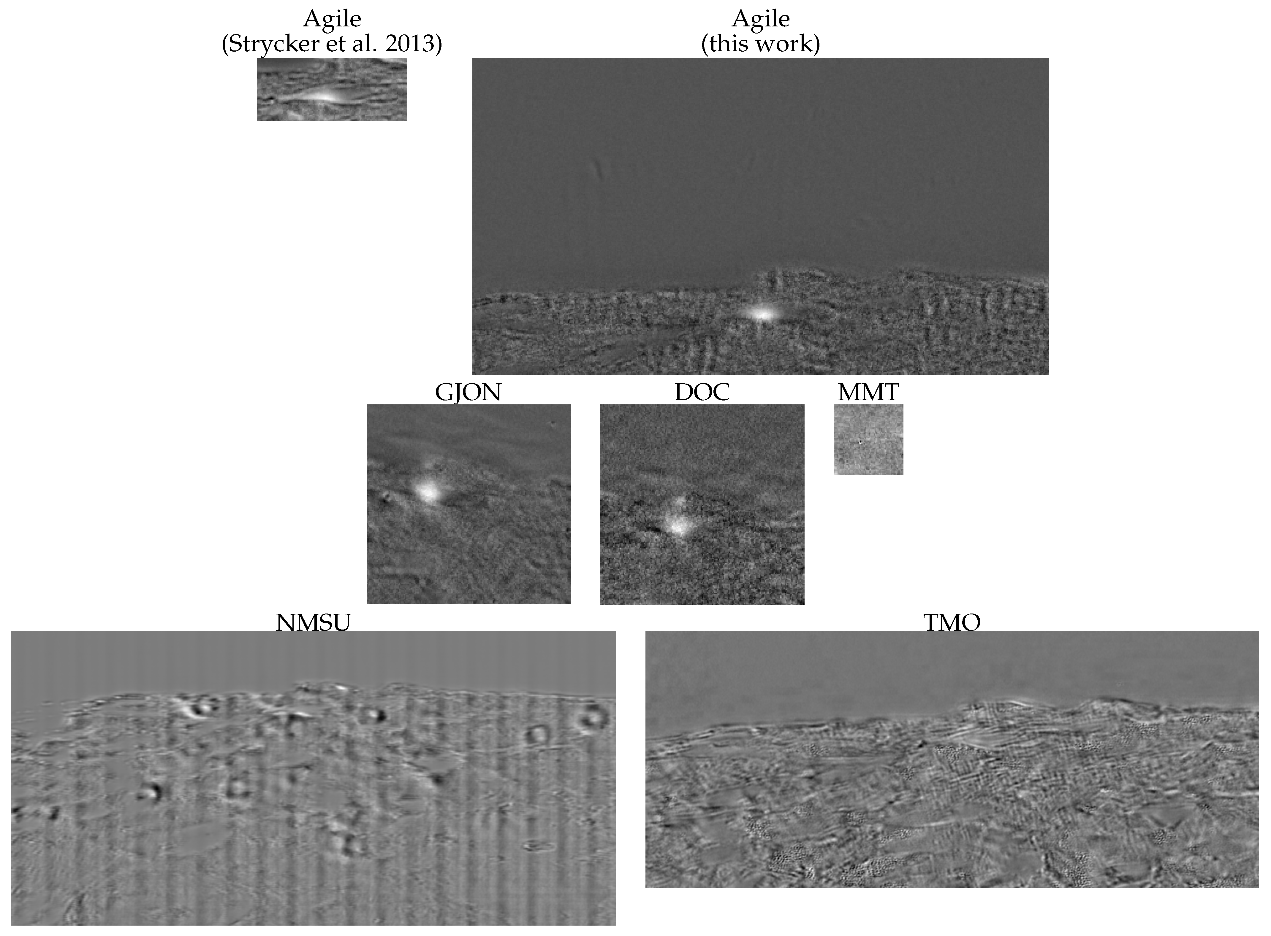
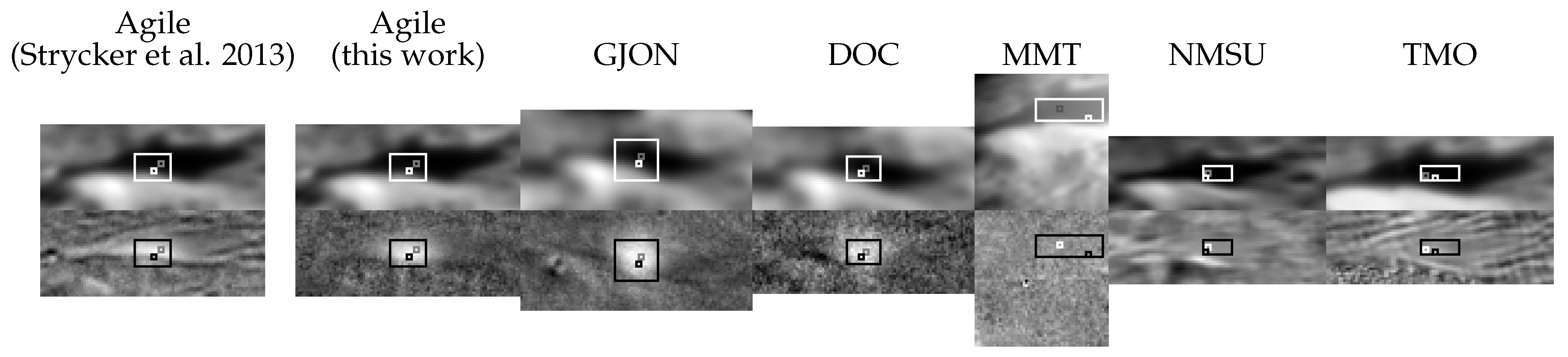
The search for pixel-specific lightcurves of the LCROSS plume consisted in finding a way to effectively remove the Moon from the data. If the lunar signal were unchanged by the turbulent atmosphere, drifting rotation of the FOV (due to slight mismatch between the target’s changing position angle caused by Earth’s rotation relative to the target and the observer’s preset mechanical derotation rate of the optical port that mounts the camera to the telescope that is intended to offset this effect), and imperfect coregistration, then removing PC1 from the data would cleanly remove the static lunar signal, though not its shot noise. In the actual situation, removing PC1 alone will leave residual counts wherever that frame’s landscape was blurrier, sharper, warped, shifted, or rotated compared to PC1. As more atmospheric and full-frame-correcting PCs are included with PC1, their sum will increasingly match and remove the lunar signal actually detected (see Figure 3, Figure 4, Figure 5 and Figure 6).

PCA ranks PCs by the amount of variance they account for in the time series from greatest to least. The data sets considered here have variance dominated by the high counts in the illuminated lunar surface (see

Table 2. Characteristics of each data set prior to PCA filtering measured over the total observation duration. Full-frame scattered light is measured at the maximum SNR pixel (see Figure 4). Illuminated surface values are from the pixel of maximum brightness in the foreground ridge obscuring the impact site, which is the brightest illuminated surface in the vicinity of Cabeus. (This feature is necessarily within the FOV for observations designed to view ejecta at the lowest possible altitudes). We overestimate the SNR here by assuming that the illuminated surface has a signal strength equal to the dynamic range and is affected by Poisson noise only. Values marked in bold likely account for the non-detection in that data set.

Data Set	Agile	GJON	DOC	MMT	NMSU	TMO
Illuminated Surface (counts)	58,325	10,359	1555	13,620	1520	228
Full-frame Scattered Light (counts)	4274	2204	341	8318	45	41
Dynamic Range (counts)	54,051	8155	1214	5302	1475	187
SNR of Illuminated Surface	232	90	35	73	38	14
Dynamic Range/Full-frame Scattered Light	12.6	3.7	3.6	0.6	33	4.6
Wavelength Band (to indicate solar insolation)	V	visible	visible	0.7 μm	R	J & H
Total Usable Frames	1937	12,962	12,970	17,986	3598	13,406

), a significant fraction of which would be displaced into neighboring pixels by atmospheric and even subtle full-frame changes (e.g., rotation and misalignment). Thus, these effects are the lowest-order PCs. It follows that the SNR of faint, non-lunar sources’ lightcurves will increase by removing the lowest-order PCs.

Strycker et al. [13] adopted the policy of removing only those PCs whose meanings were fully understood. Their primary reason was to unambiguously demonstrate the validity of the PCA filtering method by producing a detection with the fewest possible assumptions. Our goal in this work is to find the maximum possible SNR for the LCROSS plume and, thereby, to demonstrate the full power of PCA filtering. We approach this maximization problem with a computationally expensive, brute force method: cumulative sequential elimination (CSE) of PCs from the reduced time series.

By PCA filtering a growing set of PCs—PC1, then PCs 1–2, then PCs 1–3, etc.—and retrieving a plume lightcurve after each set, we achieve a gradual increase in the plume’s SNR leading up to the higher-order PCs that begin describing the plume itself. The large bottom panel of Figure 5 demonstrates this CSE improvement of the SNR of the plume detection followed by gradual loss of SNR. In this work, we employed the known times and positions of the expected transient counts in the CSE-based search for a maximum SNR. We did not need to develop an algorithm to search for unknown transient events across all times and positions. Such algorithms for applying PCA filtering to the fullest extent with CSE for blind transient detection is an area of future work. Here, we saved computation complexity, time, and memory by saving the average SNR of each pixel’s lightcurve during just the span of significant plume brightness for each step of CSE. This allowed us to discard the hundreds of large intermediate output files that would otherwise be necessary to keep for an exhaustive search for transients.

After each CSE step, the newly PCA-filtered time series was processed to find the SNR of the plume signal in every pixel. Regardless of the frame cadence (see Table 1), we applied a 2.5 s boxcar average to decrease the shot noise. Next, we chose to average post-impact times from 15–33 s to quantify the plume signal, based on the plume lightcurve in the Strycker et al. [13] reduction of Agile data. The goal of CSE for detections was to see the gradual maximization of SNR, so it was appropriate to use a larger window of time for averaging the signal to encompass more of the lightcurve than just the peak brightness from 17–23 s. We quantified the noise by calculating the standard deviation of each pixel’s lightcurve during the final 40 s prior to impact to match the approximate duration of post-impact excess brightness. Throughout this work, we assume the definition of SNR to be average signal counts divided by the standard deviation of these pre-impact counts.

The boxcar average was not strictly necessary for our CSE search—the plume signal averaged from 15 to 33 s is not significantly affected by it. However, the standard deviation is greatly affected by the boxcar average. Therefore, we performed it to maintain methodological consistency with the final reduced data products that we chose to create after being guided by the SNR found by CSE.

We used the SNR results from CSE to determine the maximum number of lowest-order PCs to remove from each data set. Figure 3, Figure 4, Figure 5 and Figure 6 and

Table 3. Characteristics of each PCA-filtered data set and resulting plume detection. ^† Averaged across the region indicated in Figure 4 over post-impact times from 17 to 27 s in the PCA-filtered data. The values reported for non-detections indicate the excess brightness in this region due to random fluctuations over this time span and not from a plume-like lightcurve. ^‡ The peak plume brightness is the maximum value of excess brightness in counts from a single pixel (see Figure 4) at a single frame after the application of the 2.5 s boxcar average used in all post-PCA filtering analyses. * We calculated standard deviation from a pixel’s or region’s lightcurve during the final 40 s prior to impact to match the approximate duration of post-impact excess brightness. We assume this definition for all subsequent tables and figures.

	Detection			Non-Detection
Data Set	Agile	GJON	DOC	MMT	NMSU	TMO
Total Number of Frames and, therefore, PCs	1937	12,962	12,970	17,986	3598	13,406
Highest PC Removed for PCA Filtering	46	46	20	23	22	150
Percent of PCs Removed for PCA Filtering	2.37%	0.35%	0.15%	0.13%	0.61%	1.12%
Excess Brightness of Plume Location † (counts)	158.7	25.0	6.4	4.4	3.8	0.4
Peak Plume Brightness ‡ (counts)	436.6	65.2	15.5	-	-	-
SNR of Plume Location † (standard deviations) *	6.2	5.6	3.8	0.3	2.2	1.2
Dynamic Range/Plume Brightness †	341	326	190	-	-	-
Dynamic Range/Peak Plume Brightness ‡	124	125	78	-	-	-

provide the detailed results: Figure 3 shows the spatial extent of peak plume brightness, Figure 4 highlights the pixels selected for representative lightcurves and quantifying detection strengths, Figure 5 explores the choice of PCs for PCA filtering, and Figure 6 contains the final PCA-filtered lightcurves.

Figure 5 shows two ways by which we ensured that the SNR-maximizing set of PCs filtered was not spurious. First, in the large bottom panel with SNR versus PCs removed, we gained confidence in our choice if the CSE progression reached a global SNR maximum by an incremental rise and then fall without competing similar features reaching comparable maxima elsewhere. Second, using the camera-specific lightcurves in the upper panels that show the progression of lightcurve shape with CSE, we checked that the shape did not exhibit a dramatic change with a PCA filtering choice in the PCs immediately leading up to the maximum SNR that are comparable in SNR. For example, it would lower our confidence in picking PCs 1–46 if removing PC46 makes a big difference in shape and removing PCs 1–44 would achieve a SNR almost as good. For each data set with a plume detection, the SNR-maximizing set of PCs was not spurious and was chosen to produce the final PCA-filtered data (see Table 3). For all data sets, including the non-detections, we applied the 2.5 s boxcar average as a last reduction step.

4. Results

With the above methodology, we unambiguously detected the LCROSS plume in the Agile, GJON, and DOC data sets (see Section 4.1). The non-detections in the MMT, NMSU, and TMO data sets are characterized in Section 4.2. Our inability to detect the plume in these data sets is explored through synthetic degradation of detection data in Section 4.3.

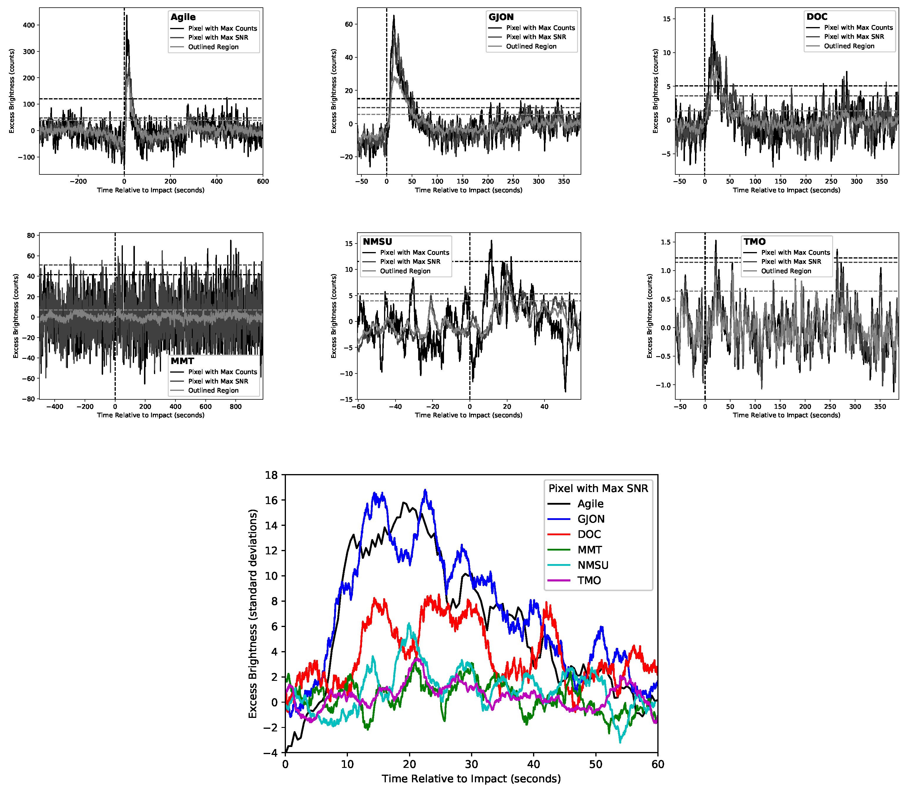
4.1. Plume Lightcurves

The increased FOV analyzed, increased timespan analyzed, and improved PCA filtering methods used in this work yielded a higher SNR detection of the debris plume in the Agile data compared to that of Strycker et al. [13]. Figure 7 shows the lightcurves for the timespan analyzed by each as well as a closer view of the first minute after impact. Averaged across 140 pixels covering the central debris plume over post-impact times from 17–27 s, the re-reduced data had a single-pixel SNR of 6.2σ (see Table 3), whereas Strycker et al. [13] had a single-pixel SNR of 3.9σ. This enabled a modeling analysis of the data by Luchsinger et al. [18] with a higher spatial resolution compared to the 4 × 4 binning used by Strycker et al. [13]. Luchsinger et al. [18] used the gains in SNR and spatial resolution to extend the modeling parameters to include particle albedo as a function of lunar sediment depth and to retrieve the separate water and regolith contents in the pre-impact lunar sediment. These additional scientific insights were not possible with the older data.

We confirm plume detections with both the GJON and DOC cameras that are consistent with the Agile detection. The GJON detection is 1.5 times stronger on average than the SNR of the DOC detection (see Table 3). The GJON detection is comparable to the SNR of the Agile detection throughout the first minute after impact (see Figure 6). In the lightcurves that are averaged over the plume regions (Figure 6, light gray curves), the GJON and DOC detections match the rapid rise of the Agile detection in brightness around 10 s relative to impact, a prolonged high SNR level from 15–25 s, and then a gradual decline in brightness reaching 50% around 33 s.

The average spatial distributions of the detections in Figure 3 match visually between all three data sets. The detections described in this work extend farther and compete with fewer lunar features with spurious excess brightness than the Strycker et al. [13] detection (Figure 3, top left). It is also noteworthy that the locations identified in Figure 4 for the maximum SNR pixels is a dark position in Cabeus along the vertical path of ejecta, while the locations for the maximum count pixels is the position in Cabeus nearest the impact and above the foreground ridge.

4.2. Non-Detections

For each data set with a non-detection, the plot of SNR versus PCs removed (Figure 5, bottom) contained only very weak features, with the exception of the initial steady decrease in SNR for the MMT data. This was due to the use of MMT’s adaptive optics. The lack of both PSF and geometry variations in the MMT data leads to no PCs beyond PC1 that can be removed to better account for the unwanted lunar signal. Because there was no obvious set of PCs that would yield a detection for MMT, NMSU, and TMO data, we visually inspected the CSE results—i.e., the spatial image of the signal averaged over 15–33 s—over the entire PC search span: CSE from 1–100 for NMSU and TMO and CSE from 1–500 for MMT. None of the non-detections we report had a plume-like spatial shape to the 15–33 s signal, nor did they have signal levels in Cabeus crater that exceeded the levels at other locations in the FOV. Finally, we inspected the lightcurves at the pixel with the maximum SNR (Figure 5, bottom row of panels) and found no indication of a plume-like lightcurve shape at any step along the CSE. NMSU data were searched again with the further constraint of using the signal averaged from 17–23 s, which was the peak of brightness in the detections. This did not yield a detection.

Our choice of PCs to remove for the final PCA-filtered data became somewhat arbitrary for these non-detections. We chose the global maximum in SNR for the NMSU data and a local maximum for the MMT data. We chose to remove PCs 1–150 for the TMO data, which was beyond the CSE search from PCs 1 to 100, because its SNR seemed to have a positive slope near PC100 without having reached a clear global maximum. This extended CSE search was only for the sake of completeness; the data themselves did not give reason to believe that a plume signal was emerging, as can be seen from the CSE lightcurves for TMO data in Figure 5.

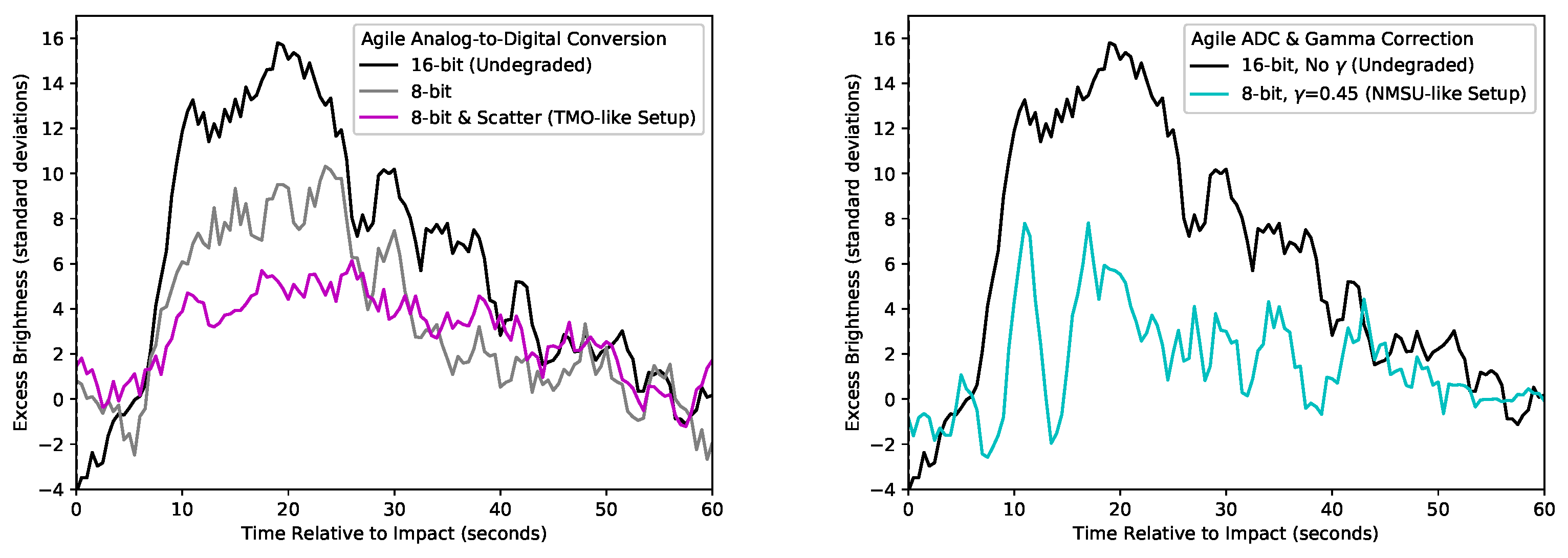
4.3. Lightcurve Retrievals from Degraded Detection Data

Our first step to understanding the non-detection data was to find the practical limits of detection with PCA filtering. We took the data containing detections and then degraded a specific factor by progressively greater amounts until either the plume was no longer detectable or the factor was degraded beyond a reasonable limit. In this manner, we explore the effects of additional scattered light, worse atmospheric seeing, and longer exposures in Section 4.3.1. In Section 4.3.2, we degrade the data’s digital resolution in the ADC by reducing the number of bits and by removing its linearity through gamma compression.

4.3.1. Effects of Scattered Light, Atmospheric Seeing, and Exposure Time

We used all three data sets with detections to investigate the effects of degrading three basic observing parameters. The detection strength versus initial parameter values of scattered light, atmospheric seeing, and integration time for exposures for each data set are represented as solid circles in the top row of panels in Figure 8. We synthetically degraded each parameter independently, performed PCA on the degraded data, searched for a maximum SNR plume signal with CSE, and extracted the excess brightness averaged over 15–33 s from the 2.5 s boxcar averaged maximum SNR lightcurve. The results from degraded parameter values are shown as open circles in Figure 8.

We added full-frame scattered light by initializing an array of the desired constant value for every frame in the time series, generating Poisson noise unique to each pixel and frame, and adding the resulting arrays to the coregistered time series. In order to compare scattered light results across all data sets, we needed a metric for the relative amount of full-frame scattered light in each. We first found the dynamic range for each data set, defined as the count level in the darkest unilluminated portion of Cabeus subtracted from the count level of the brightest illuminated surface of the foreground ridge obscuring the impact site. Then we divided this dynamic range by the full-frame scattered light, defined as the count level in the darkest unilluminated portion of Cabeus. As we added full-frame scattered light, the dynamic range stayed constant and the ratio of dynamic range to full-frame scattered light—our metric—decreased.

These results are given in the left panels of Figure 8. As the metric decreased leftward on the x-axis, the PCA methodologies we used were progressively less successful at separating the plume signal from the Poisson noise. The Agile data lightcurves from the maximum SNR pixel in the bottom panel demonstrate the effects on the lightcurve shape. We note that GJON data lose detectability slower than Agile and DOC data, which were roughly equivalent in their loss of detectability with respect to our metric. We speculate that the reason for the greater robustness against Poisson noise of plume retrievals in GJON data may be a combination of its higher SNR than DOC data and its much higher frame cadence than Agile data, giving the GJON data many more PCs to work with.

Increasing the full-width-at-half-maximum (FWHM) of the seeing required a convolution with a Gaussian PSF. Although the spatial information present in the data suffered a corresponding loss of resolution, this made very little difference in the retrieval of temporal information, as shown in the middle panels of Figure 8. In fact, the GJON and DOC detections increased SNR slightly with small increases in FWHM and the plume was still detectable after the FOV appeared nearly uniform. We conclude that spatial resolution itself is not a limiting factor in the PCA filtering methodology. Defocusing is a known technique for increasing the accuracy of stellar photometry [19]. Our result demonstrates this technique’s feasibility for relative photometry of a transient source in a crowded field or with spatially extended background sources. Although coregistration of the raw time series would become degraded as spatial resolution decreased (which is an effect beyond the scope of this work), the transient signal is spread by the seeing to the same extent as the static background. From the results for FWHM > 8 arcsec, we expect that the plume should be detectable without coregistration if the telescope pointing is consistently within an arcsec across the duration of the time series.

Increasing the integration time of each exposure required rebinning the temporal dimension of each data set. This process is not the same as the time averaging applied to the undegraded data for the actual detections. The 2.5 s boxcar averaging was done post-PCA so that all non-averaged frames are included in PCA, whereas this degrading process reduces the number of raw frames going into the PCA, thus reducing the number of PCs generated. The right panels of Figure 8 show the results. The GJON detection increased SNR slightly and the SNR of the DOC detection more than doubles with integration times approximately equal to the duration of the peak brightness of the plume. The plume is still detectable in all three data sets with 30 s integration times. We suspect that Nyquist sampling rate (i.e., a frame cadence greater than twice the duration of the transient) and CCD saturation considerations are likely to limit integration times, as opposed to a loss of detectability with PCA filtering methodology.

4.3.2. Effects of ADC Reduction to 8-Bit and Gamma Correction

We used the Agile data to investigate the effects of degraded digital resolution. First, it is the most thoroughly characterized detection. Second, it contains the greatest number of counts in the plume signal. Third, its high number of counts in the raw data allowed us more control in altering its ADC. For the sake of explaining the NMSU and TMO non-detections (see Section 5), we matched the raw counts at one or more positions in the lunar landscape in NMSU and TMO data to the same positions in these ADC degraded Agile data.

In the left panel of Figure 9, we see a loss of almost half the SNR of the plume when switching from 16-bit to 8-bit ADC resolution. Furthermore, the SNR of the plume is strongly affected by additional scattered light. The ratio of dynamic range to full-frame scattered light of the Agile data is 12.6 (Figure 9, gray line), and we added full-frame scattered light to match the ratio of 4.6 in the TMO data (Figure 9, magenta line). The TMO-like setup has a lower SNR than we would expect with 16-bit ADC due to scattered light alone from the upper left panel of Figure 8.

The loss of SNR is even larger when gamma compression is used, as evidenced by the right panel of Figure 9. This makes sense considering the antithetical natures of gamma compression and PCA: non-linear and linear, respectively. Under gamma compression, each incremental step up requires a larger number of electrons (linear counts) added to the pixel than the previous step. Although gamma compression thereby allows for raw detection of small variations in pixels with low count levels, variations up and down are asymmetric. Consider a linear variation that moves the time averaged pixel value down one gamma step. A variation up with the same linear size will not move the same time averaged pixel value up one gamma step. However, PCA provides a new set of base vectors (PCs) that are linearly added and subtracted from one another to fully represent the data. Given the gamma-induced asymmetry, PCs become less efficient at describing lightcurve correlations in the data.

Gamma correction also prevents the possibility of the correlation of lightcurve variations across the full FOV. For example, given gamma correction and a small change in seeing, the high count landscape positions might stay at their values or go down a large gamma step as light spreads away from them while the low count positions into which light is spread will gain many smaller gamma steps. Thus, for many causes of temporal variations, only positions with similar count levels will experience effects of the same magnitude. The disparities introduced by gamma correction between contrasting count levels across the FOV will weaken or erase correlations from the data. These lines of reasoning seem sufficient to explain the poor performance of PCA filtering with gamma corrected data.

5. Discussion

A major goal of this work is to identify factors that influence the detectability of LCROSS-like events (i.e., low SNR transients) and to establish practical constraints and preparatory steps for observing. Factors we considered are listed in

Table 4. A comparison of possible detectability factors for each data set. Values marked in bold likely account for the non-detection in that data set. ^† Averaged across the region indicated in Figure 4 over post-impact times from 17 to 27 s in the PCA-filtered data. The values reported for non-detections indicate the level of excess light in this region over this time span due to random fluctuations and not from a plume-like lightcurve.

	Detection			Non-Detection
Data Set	Agile	GJON	DOC	MMT	NMSU	TMO
Excess Brightness of Plume Location † (counts)	158.7	25.0	6.4	4.4	3.8	0.4
SNR of Plume Location † (standard deviations)	6.2	5.6	3.8	0.3	2.2	1.2
Dynamic Range/Plume Brightness †	341	326	190	-	-	-
Dynamic Range/Peak Plume Brightness	124	125	78	-	-	-
Dynamic Range/Full-frame Scattered Light	12.6	3.7	3.6	0.6	33	4.6
SNR of Illuminated Surface	232	90	35	73	38	14
ADC Resolution	16-bit	16-bit	16-bit	16-bit	8-bit	8-bit
ADC Gamma Correction	-	-	-	-	0.45	-
Wavelength Band (to indicate solar insolation)	V	visible	visible	0.7 μm	R	J & H
Neutral Density or U Filter	ND2.5	U	U	ND2.5	-	-
Lunagraph (to reduce scattered light)	Yes	-	-	-	-	-
Telescope Diameter (m)	3.5	2.4	2.4	6.5	1.0	0.6
Adaptive Optics	-	-	-	Yes	-	-
Seeing Point Spread Function (arcsec)	0.8–1.4	2	2	0.38	0.8–1.4	1
Image Scale (arcsec pixel−1)	0.26	0.27	0.29	0.27	0.28–0.33	0.22
Image Scale at Lunar Distance (km pixel−1)	0.46	0.49	0.51	0.48	0.51–0.60	0.39
Dimensions of Usable Image (pixels)	466 × 256	165 × 161	165 × 162	57 × 56	643 × 313	652 × 273
FOV at Lunar Distance (km)	214 × 118	80 × 78	84 × 83	27 × 27	328 × 188	254 × 106
Frame Integration Time (s)	0.5	0.032	0.032	0.071	0.001	0.019
Frame Cadence (s)	0.5	0.034	0.034	0.079	0.033	0.033
Total Usable Frames	1937	12,962	12,970	17,986	3598	13,406
Total Observation Duration (s)	968	442	442	1482	120	447

. Capitalizing on the detection data, we verify that some degraded conditions result in the loss of detectability with our PCA filtering and CSE methodologies: full-frame scattered light that greatly exceeds the dynamic range, low digital (ADC) resolution, and deviation from detector linearity through gamma correction. We also found that detectability is robust against worsening seeing and protracted integration times. We now apply these findings to the MMT, NMSU, and TMO data and, where necessary, search for additional reasons for their non-detections.

The strongest connection is the small ratio of dynamic range to full-frame scattered light in the MMT data (Figure 8, left panels) compared to the other five data sets, whereas it compares favorably—with the exception of its small FOV—to the detections in all other factors listed in Table 4. We interpret this to mean that the shot noise from the scattered light overwhelmed the plume signal, which would have had a lower SNR than Agile and GJON data due to the smaller SNR for the illuminated surface in MMT data. Our tests with degraded seeing give credibility to our belief that the excellent seeing from MMT’s adaptive optics was not a sufficient counter-measure to the excess of full-frame scattered light.

We suspect that the non-detectability of a plume in the NMSU data was primarily due to the gamma correction, secondarily to the 8-bit ADC, and lastly to the SNR for the illuminated surface. These three work in concert against the ability of PCA to discriminate between underlying causes of lightcurve variations at low count levels. We reiterate our reasoning above (Section 4.3.2) for placing gamma correction first in the list: PCA is a linear analysis and gamma compression weakens lightcurve correlations. The problem is exacerbated by low digital resolution and low SNR in the raw data. The lunar landscape had a SNR of 38 in the NMSU data, which is slightly higher than in the DOC data (35, the weakest of the detections), yet the NMSU data were acquired through the use of gamma correction in order to achieve this SNR.

The TMO data non-detection is also not due to a single factor. We first note that our plume detections were all at visible wavelengths, so we do not precisely know what strength the plume signal had in the J and H bands of the observations made with TMO. The TMO-like setup of degraded APO data (Figure 9, magenta line) shows the possibility of a visible-band plume detection despite its 8-bit ADC. TMO data, however, had an SNR for the illuminated surface of only 14, which is less than half of the DOC data SNR and more than 16 times smaller than the Agile data SNR.

Considering the above explanations for non-detection, we raise the question of the possibility of a detectable LCROSS plume in other data sets. Given low enough levels of scattered light, high enough SNR of illuminated lunar surface, and high enough ADC resolution that preserves the detector’s linearity, appropriate data could have been collected at any spatial or temporal resolution. This suggests that across the wide range of observers who supported the LCROSS event—from research observatories to the amateur astronomy community—it is possible that some achieved this without knowing it. We encourage the reanalysis of privately archived data with the methods presented here.

6. Conclusions

We improve data reduction methodologies for time series imaging with PCA filtering. As opposed to statistical analyses that reduce the dimensionality of the data (e.g., mean and median), PCA is a synthesis of all the information present—each of its re-oriented dimensions (PCs) depends on the information in all the others. We stress that making use of even a single PC means that every datum in the time series has been taken into account in a way that respects the reality that each datum was the sum total of statistically independent processes.

By taking all spatial and temporal signals into account, and not just those of the sharpest subset of images, the coregistration process benefits from PCA-filtered fiducial reference images. These contain less noise than the median of a subset of images while accurately exhibiting the average geometry of the time series with better than average seeing. This results in higher probabilities for correct alignment across all images, giving the low SNR transients within the time series an increased detectability.

We use PCA filtering to effectively remove a static background signal that is spatially and temporally modified by atmospheric and instrumental effects. We iteratively remove PCs from the data through CSE to find a maximum SNR of the LCROSS ejecta plume signal. The CSE approach demonstrates significant SNR gains over the Strycker et al. [13] conservative method of removing only PCs fully understood (i.e., recreatable with synthetic observations).

With these methods, we confirm and strengthen the Strycker et al. [13] detection made with the Agile instrument at the APO 3.5 m telescope and discover two additional detections made with the GJON and DOC cameras mounted on a two-channel dichroic at the MRO 2.4 m telescope. All three detections are in mutual agreement concerning the plume lightcurve and spatial extent. We report three non-detections from data acquired with the NMSU 1.0 m telescope at APO, the TMO 0.6 m telescope, and the 6.5 m MMT.

Finally, we evaluate the criteria for detectability in future observations of low SNR transient events. Our results indicate three observational setup constraints for the practical success of PCA filtering: (1) full-frame scattered light should not exceed the dynamic range between the illuminated and unilluminated surfaces, (2) the camera’s ADC should use at least 16-bit resolution, and (3) the ADC should not use gamma correction. We find that poor spatial or temporal resolution do not significantly degrade detectability. This suggests that future LCROSS-like events and natural transient phenomena—such as bolides in distant planetary atmospheres and lunar impact flashes—may be more detectable in amateur observations with PCA filtering.

References

1. Colaprete, A.; Schultz, P.; Heldmann, J.; Wooden, D.; Shirley, M.; Ennico, K.; Hermalyn, B.; Marshall, W.; Ricco, A.; Elphic, R.C.; et al. Detection of Water in the LCROSS Ejecta Plume. Science 2010, 330, 463. [Google Scholar] [CrossRef] [PubMed] [Green Version]
2. Schultz, P.H.; Hermalyn, B.; Colaprete, A.; Ennico, K.; Shirley, M.; Marshall, W.S. The LCROSS Cratering Experiment. Science 2010, 330, 468. [Google Scholar] [CrossRef] [PubMed]
3. Feldman, W.C.; Maurice, S.; Binder, A.B.; Barraclough, B.L.; Elphic, R.C.; Lawrence, D.J. Fluxes of Fast and Epithermal Neutrons from Lunar Prospector: Evidence for Water Ice at the Lunar Poles. Science 1998, 281, 1496. [Google Scholar] [CrossRef] [PubMed] [Green Version]
4. Feldman, W.C.; Lawrence, D.J.; Elphic, R.C.; Vaniman, D.T.; Thomsen, D.R.; Barraclough, B.L.; Maurice, S.; Binder, A.B. Chemical information content of lunar thermal and epithermal neutrons. J. Geophys. Res. Planets 2000, 105, 20347–20364. [Google Scholar] [CrossRef]
5. Feldman, W.C.; Maurice, S.; Lawrence, D.J.; Little, R.C.; Lawson, S.L.; Gasnault, O.; Wiens, R.C.; Barraclough, B.L.; Elphic, R.C.; Prettyman, T.H.; et al. Evidence for water ice near the lunar poles. J. Geophys. Res. Planets 2001, 106, 23231–23252. [Google Scholar] [CrossRef]
6. Colaprete, A.; Elphic, R.C.; Heldmann, J.; Ennico, K. An Overview of the Lunar Crater Observation and Sensing Satellite (LCROSS). Space Sci. Rev. 2012, 167, 3–22. [Google Scholar] [CrossRef]
7. Boazman, S.; Kereszturi, A.; Heather, D.; Sefton-Nash, E.; Orgel, C.; Tomka, R.; Houdou, B.; Lefort, X. Analysis of the Lunar South Polar Region for PROSPECT, NASA/CLPS. In Proceedings of the Europlanet Science Congress, Granada, Spain, 18–23 September 2022; p. EPSC2022-530. [Google Scholar] [CrossRef]
8. Heldmann, J.L.; Colaprete, A.; Wooden, D.H.; Ackermann, R.F.; Acton, D.D.; Backus, P.R.; Bailey, V.; Ball, J.G.; Barott, W.C.; Blair, S.K.; et al. LCROSS (Lunar Crater Observation and Sensing Satellite) Observation Campaign: Strategies, Implementation, and Lessons Learned. Space Sci. Rev. 2012, 167, 93–140. [Google Scholar] [CrossRef] [Green Version]
9. Heldmann, J.L.; Lamb, J.; Asturias, D.; Colaprete, A.; Goldstein, D.B.; Trafton, L.M.; Varghese, P.L. Evolution of the dust and water ice plume components as observed by the LCROSS visible camera and UV-visible spectrometer. Icarus 2015, 254, 262–275. [Google Scholar] [CrossRef]
10. Killen, R.M.; Potter, A.E.; Hurley, D.M.; Plymate, C.; Naidu, S. Observations of the lunar impact plume from the LCROSS event. Geophys. Res. Lett. 2010, 37, L23201. [Google Scholar] [CrossRef]
11. Chanover, N.J.; Miller, C.; Hamilton, R.T.; Suggs, R.M.; McMillan, R. Results from the NMSU-NASA Marshall Space Flight Center LCROSS observational campaign. J. Geophys. Res. Planets 2011, 116, E08003. [Google Scholar] [CrossRef]
12. Hong, P.K.; Sugita, S.; Okamura, N.; Sekine, Y.; Terada, H.; Takatoh, N.; Hayano, Y.; Fuse, T.; Pyo, T.S.; Kawakita, H.; et al. A ground-based observation of the LCROSS impact events using the Subaru Telescope. Icarus 2011, 214, 21–29. [Google Scholar] [CrossRef]
13. Strycker, P.D.; Chanover, N.J.; Miller, C.; Hamilton, R.T.; Hermalyn, B.; Suggs, R.M.; Sussman, M. Characterization of the LCROSS impact plume from a ground-based imaging detection. Nat. Commun. 2013, 4, 2620. [Google Scholar] [CrossRef] [PubMed] [Green Version]
14. Murtagh, F.; Heck, A. Multivariate Data Analysis; Springer: Berlin/Heidelberg, Germany, 1987; Volume 131, ISBN 978-94-009-3789-5. [Google Scholar] [CrossRef]
15. Mukadam, A.S.; Owen, R.; Mannery, E.; MacDonald, N.; Williams, B.; Stauffer, F.; Miller, C. High-Speed Time-Series CCD Photometry with Agile. Publ. Astron. Soc. Pac. 2011, 123, 1423. [Google Scholar] [CrossRef]
16. Young, E.F.; Young, L.A.; Olkin, C.B.; Buie, M.W.; Shoemaker, K.; French, R.G.; Regester, J. Development and Performance of the PHOT (Portable High-Speed Occultation Telescope) Systems. Publ. Astron. Soc. Pac. 2011, 123, 735. [Google Scholar] [CrossRef] [Green Version]
17. Ennico, K.; Shirley, M.; Colaprete, A.; Osetinsky, L. The Lunar Crater Observation and Sensing Satellite (LCROSS) Payload Development and Performance in Flight. Space Sci. Rev. 2012, 167, 23–69. [Google Scholar] [CrossRef] [Green Version]
18. Luchsinger, K.M.; Chanover, N.J.; Strycker, P.D. Water within a permanently shadowed lunar crater: Further LCROSS modeling and analysis. Icarus 2021, 354, 114089. [Google Scholar] [CrossRef]
19. Southworth, J.; Hinse, T.C.; Jørgensen, U.G.; Dominik, M.; Ricci, D.; Burgdorf, M.J.; Hornstrup, A.; Wheatley, P.J.; Anguita, T.; Bozza, V.; et al. High-precision photometry by telescope defocusing—I. The transiting planetary system WASP-5. Mon. Not. R. Astron. Soc. 2009, 396, 1023–1031. [Google Scholar] [CrossRef]
Figure 1. The static lunar landscape for each data set, including the Strycker et al. [13] reduction of Agile data. These are the PC1 pixel amplitudes, which show the typical quality of seeing across each time series but with greatly reduced contamination from noise and geometric distortions.
Remotesensing 15 00037 g001
Figure 2. Flowchart of coregistration employing a PCA-filtered reference image. The Python code we developed for this process (coreg_pca in image_cube.py) is available in Zenodo at https://doi.org/10.5281/zenodo.7268912.
Remotesensing 15 00037 g002
Figure 3. The PCA-filtered data averaged over post-impact times from 17 to 27 s reveal plume detections in Agile, GJON, and DOC. The Strycker et al. [13] data reduction is included for comparison.
Remotesensing 15 00037 g003
Figure 4. Pixel locations used in analyses overlaid on cropped images of PC1 (top row) and the average PCA-filtered data over post-impact times from 17 to 27 s (bottom row). The individual pixel outlined in gray in each PC1 image contains the maximum SNR of excess brightness averaged over post-impact times from 15 to 33 s. The individual pixel outlined in white in each PC1 image contains the maximum counts of excess brightness. The outlined region contains the central area of the plume detections for the Strycker et al. [13] Agile data reduction, Agile (this work), GJON, and DOC. For the non-detections of MMT, NMSU, and TMO, the outlined region had the highest likelihood for potential detections.
Remotesensing 15 00037 g004
Figure 5. The small panels contain PCA-filtered lightcurves from CSE. These show excess counts for the first minute after impact at the maximum SNR pixel (see Figure 4) with a 2.5 s boxcar average (We assume the use of PCA-filtered data with a 2.5 s boxcar average for all subsequent figures). The lightest shade of gray is PCA filtering by removing only PC1, and shading darkens with increasingly higher PCs filtered in CSE. The line becomes black when PCs 1–100 are removed for all cameras except for TMO, for which black represents PCs 1–300 removed. The dashed line indicates the lightcurve at the level of PCA filtering chosen based on the maximum SNR shown in the lower panel. The lower panel shows the SNR achieved through CSE of PCs from each data set. We averaged the excess brightness at the maximum SNR pixel (see Figure 4) over 15 to 33 s after impact for all cameras except for NMSU, for which we narrowed the window to 17 to 23 s after a non-detection using the broader window.
Remotesensing 15 00037 g005
Figure 6. Lightcurves retrieved with the methodology of this work from the locations indicated in Figure 4. The small panels show the total duration of each observation. The horizontal dashed lines give the 3σ level for each camera. In the lower panel, the excess brightness is shown scaled by signal strength in standard deviations for the first minute after impact.
Remotesensing 15 00037 g006
Figure 7. Comparison of the Strycker et al. [13] data reduction with that of this work. The lightcurves are from the locations indicated in Figure 4. The horizontal dashed lines give the 3σ level for each reduction.
Remotesensing 15 00037 g007
Figure 8. Maximum retrieved SNR over 15 to 33 s after impact from degraded data at the maximum SNR pixel (see Figure 4). From left to right, these are results for additional scattered light, worsened atmospheric seeing, and longer exposures. The bottom row shows lightcurves for selected data. The lightcurve for an MMT-like amount of scattered light does not fully characterize MMT because it does not take other factors into account (e.g., the fact that the dynamic range of MMT data was smaller than that of Agile data).
Remotesensing 15 00037 g008
Figure 9. SNR retrieved for Agile data degraded with 8-bit resolution (left) and both 8-bit resolution and gamma correction (right) at the maximum SNR pixel (see Figure 4). The TMO-like setup (magenta line) shows the possibility of a visible-band plume detection with an observational setup similar to that of TMO. TMO, however, did not achieve a high SNR of the illuminated lunar landscape before the ADC process, unlike the degraded Agile data here. Thus, the magenta line ought to have a greater SNR than any plume signal in the TMO data. The cyan line in the right panel is degraded to 8-bit resolution with gamma correction of 0.45 and the dynamic range adjusted to match that of the NMSU data.
Remotesensing 15 00037 g009