Abstract
Climatic variability and the quantification of climate change impacts on hydrological parameters are persistently uncertain. Remote sensing aids valuable information to streamflow estimations and hydrological parameter projections. However, few studies have been implemented using remote sensing and CMIP6 data embedded with hydrological modeling. This research studied how changing climate influences the hydro-climatic parameters based on the earth system models that participated in the sixth phase of the Coupled Model Intercomparison Project (CMIP6). GRACE evapotranspiration data were forced into the Soil and Water Assessment Tool (SWAT) to project hydrologic responses to future climatic conditions in the Hongshui River basin (HRB) model. A novel approach based on climate elasticity was utilized to determine the extent to which climate variability affects stream flow. CMIP6 SSPs (shared socio-economic pathways) for the second half of the 20th century (1960–2020) and 21st century (2021–2100) projected precipitation (5–16%) for the whole Hongshui River basin (HRB). The ensemble of GCMs projected an increase of 2 °C in mean temperature. The stream flow is projected to increase by 4.2% under SSP-1.26, 6.2% under SSP-2.45, 8.45% under SSP-3.70, and 9.5% under SSP-5.85, based on the average changes throughout the various long-term future scenarios. We used the climate elasticity method and found that climate change contributes 11% to streamflow variability in the Hongshui River basin (HRB). Despite the uncertainty in projected hydrological variables, most members of the modeling ensemble present encouraging findings for future methods of water resource management.
1. Introduction
Anthropogenic changes and the physical features of basins (such as terrain, soil, and vegetation) impact hydrological processes on a large scale. Investigating rapid changes in hydrological processes is significant due to global warming and other water-related concerns [1]. Global warming is a major obstacle and the primary source of this issue. The hydrological cycle is influenced by the average global temperature, which shifts due to changing climate [2]. The availability of water resources has been disrupted due to recent shifts in temperature and precipitation patterns and may have a significant influence on the way that local precipitation patterns form. The effect of these modifications on the hydrological cycle will either positively or negatively affect the streamflow [3]. The water resources will be impacted by several factors including but not limited to climate change, population expansion, and economic development, and researchers at the basin level are interested in these impacts. The most recent findings from scientific studies indicate that climate changes will impact hydrological processes and the total amount of water available globally [4]. During the post-impact period, climate change was responsible for 57% of the increase in streamflows over southwestern China, and human activity was responsible for 95% of the increase in streamflows (2008–2014) [5].
Throughout the last half-century in China, there has been a general decline in the runoff. The effects of human activity on runoff have been more significant than the effects of climate change [6,7,8]. Wang et al. [9] concluded that human activity had been the major factor affecting the flow in the Yellow River basin in China. Zhao et al. [10] reported that reservoir control had a more significant effect on streamflow than land-use change. Those human activities had a stronger impact on streamflow than the climatic change in the middle reaches of the Yellow River basin in China. Huang and Wang [11] studied the long-term streamflow patterns in the upper reaches of the Hongshui basin in southwest China to assess the influence of human activities and climate change on these patterns. The investigation discovered unfavorable effects for the previous 55 years such as decreased runoff. Climate is the primary driver of streamflow variance. Hydrologic sensitivity analysis evaluated that human activity and the changing climate significantly impact runoff produced in the upper reaches of the Hongshui River basin. Nonetheless, human activities between 1990 and 1999 played a critical influence in the decrease in streamflow.
Future streamflow projections using hydrological models under future climate change scenarios rely heavily on outputs from general circulation models [12,13,14]. The “Working Committee of Climate Modeling” of the Global Climate Research Program kicked up the Sixth International Coupled Model Comparison Program (CMIP6) in 2012. SSPs (shared socio-economic pathways) are used in the new socio-economic climate change scenario to illustrate the connection between radiative forcing and societal progress that follow a variety of economic and social progress trajectories. To develop more complex scenarios that consider the societal limits in climate change mitigation and adaptation, CMIP6 combines the RCPs with so-called shared SSPs. It will be a crucial source of information for the most recent IPCC report [15,16]. Many large and small basins and continental scales have been effectively modeled using CMIP6 data [17,18,19]. The combined approach of the distributed hydrological model SWAT was used with the most recently released ensemble downscaled CMIP6 outputs to project the effects of climate change on the existing hydrologic pattern in the HRB and to establish a pattern between streamflow, precipitation, temperature, and reservoir levels for each of the four shared socio-economic pathways (SSPs) (i.e., SSP-1.26, SSP-2.45, SSP-3.70, and SSP-5.85) [20,21,22].
Streamflow observations are point data, and it is not guaranteed that spatially changing water balance components like evapotranspiration are approximated successfully using simple point data at the catchment outflow for calibration. Another difficulty in hydrological model calibration is that high model performance may be achieved with a range of parameter values. The overfitting parameter is a possibility with a single-variable calibration. Some of these calibration difficulties might be alleviated by the use of several variables (such as evapotranspiration and streamflow) and multiple locations (such as streamflow data from many streams (or sub-catchments)) [23,24]. Due to the increased availability of worldwide datasets, there has been a lot of interest in incorporating two or more variables into the calibration of hydrological models. For example, several studies have made use of evapotranspiration calculations based on remote sensing [25,26,27,28,29,30], snow and glacier mass [31,32], soil moisture [33,34,35], and land surface temperature [36]. RS-based ET is one of the factors listed above that may be utilized to constrain the water balance-related hydrological modeling parameters [37,38,39]. Immerzeel and Droogers [25] found a better performance of the SWAT model calibrated with MODIS satellite evapotranspiration data. Their findings suggest that geographically dispersed ET data with a monthly temporal resolution can reduce comparable impacts from hydrological process calibration using restricted streamflow gauge data. Rientjes, Muthuwatta, Bos, Booij, and Bhatti [26] used streamflow and evapotranspiration, and their results showed that multi-variable calibration made it possible to figure out the water availability in the basin. Streamflow was replicated successfully in the single-variable calibration of a distributed hydrology model, but evapotranspiration did not perform well, and multi-variable calibration yielded more acceptable values [40]. In addition, an application of GLEAM ET revealed that calibration with more variables might assist in overcoming the problem of overparameterization [41]. Zhang et al. [42] estimated ET using GRACE (Gravity Recovery and Climate Experiment) satellite data and developed a spatial regression model of annual ET, rainfall, NDVI, and temperature. Long et al. [43] used the water balance method to derive monthly ET, whereas Zhang, Kimball, and Running [42] utilized the water balance approach to calculate the monthly ET at the continental scale by downscaling the GRACE data. GRACE data are homogeneous in scale, so there is less chance of missing data, and it can monitor changes in water storage at both the medium and large scales [44,45,46]. Numerous studies have demonstrated GRACE’s efficacy at large scale well [47,48]. Swenson, Wahr, and Milly [47] analyzed GRACE-derived regional water storage fluctuations and found that the accuracy error was less than 1 cm if the research area was more than 400,000 km2. The two most common techniques for accomplishing this reduction in spatial resolution are the dynamic downscaling approach and the statistical downscaling method. Statistical downscaling is superior to dynamic downscaling because it allows for more flexibility in model building and the use of high-resolution modeling factors, both of which increase the spatial resolution of hydrological variables [49]. GRACE and stream baseflow data were used to limit and enhance the parameter estimates in a land surface model [50]. Several studies have applied statistical downscaling based on the water balance equation approach, which successfully increased the spatial resolution [51,52,53]. Yang et al. [54] reconstructed the overall water storage anomalies using linear regression and machine learning methods, while other studies used random forest (RF) [55], multiple linear regression (MLR) [56], support vector machine (SVM) [57], and artificial neural network (ANN) [58] for long-term GRACE-derived TWS and GWS downscaling. Additionally, a few studies implemented a downscaling method that assimilated 0.5° × 0.5° water storage fields into account [52] and Arshad et al. [59] coupled downscaled-GRACE-based GWS variations with SWAT data. The results indicated that these methods could predict the time series changes, but the spatial prediction was limited. Therefore, we used a scaling factor method for increasing the GWS spatial resolution by pre-processing data combined with SWAT to improve the accuracy of hydrological modeling. It has significance and value for the study of GWS in the study area, which can be used to study the water storage in the study area and provide data support.
Reservoirs, deforestation, and soil and water conservation affect intra-annual stream flow distribution [60]. Reservoirs alter the river’s flow regime; therefore, it is natural to determine whether their construction influences the volume of runoff at the outlet [61]. For example, droughts in the Poyang Lake region have risen since the Three Gorges Dam was completed [62].
In southern China, the Hongshui River basin is the largest tributary of the Xijiang River basin and an important ecological construction target. Human activities substantially impact the Hongshui River basin’s complex climate [63]. How would the reservoirs in the HRB influence the streamflow in the context of changing climate and anthropogenic activities? Thus, it is a pressing issue that must be addressed immediately. The HRB did not experience prompt land use and development; however, policy reforms to increase economic growth, living standards, and urbanization in the early 1980s significantly affected several hydrological parameters [64,65]. Exploiting the basin’s water resources has resulted in several negative consequences on the environment and the area’s ecology including the drying up of rivers and lakes and the depletion of water levels. A further effect of the water deficit has been a rise in tension along provincial boundaries between water consumers upstream and downstream [11]. These issues are also critical to address these shortcomings, which directly affect the water resources and impact other sectors of life. However, no study has been conducted in the basin to address the quantification of streamflow using the updated version of climatic data, reservoir operation, and remotely sensed evaporation data.
The key goals of this investigation are to (1) investigate the effects of climate change on the hydrological parameters and streamflow integrating general circulation models that participated in the sixth phase of the Coupled Model Intercomparison Project (CMIP6) and GRACE data with SWAT; (2) quantify the contribution of climate change to the change in streamflow by using the climate elasticity method (CEM). This research is significant in comprehending how climate influences streamflow evolution. This study will also help policymakers understand how the streamflow responds to a changing climate and provide promising findings for future water resource management techniques.
2. Materials and Methods
2.1. Geographical Features
The Hongshui River is the primary tributary of the Xijiang River in the Pearl River basin, endowed with vast hydroelectric potential and located in southwest China, as shown in Figure 1. The drainage basin has an area of 98,500 km2 [66]. The main channel is divided into different river channels: Qianjiang, Nanpanjiang, Beipanjiang, and Hongshuihe [67]. Typically, the basin is dry and tropical, with sufficient precipitation and a high air temperature. Temperatures average between 14.5 and 22.6 °C, and yearly precipitation falls between 750 and 1800 mm. Precipitation peaks between April and October, accounting for 70–85% of annual precipitation [68]. The primary source of the Hongshui River in Qujing, Yunnan Province, is Mount Maxiong. It runs south and northeast along the boundary between Guizhou and Guangxi before entering the Beipan River. The river’s name changes to Hongshui River below this point. It then runs for 215 km in northern Guangxi until joining the main stem of the Yu River at Guiping (345 km). The Liu River, its most significant tributary, flows into it just below Laibin (Laiping). The Hongshui River and its tributaries drain almost all of southern Guizhou and northern Guangxi.
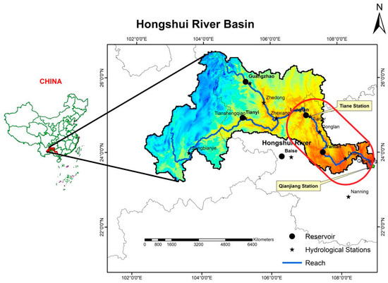
Figure 1.
Study area map of the HRB showing the major reservoirs and hydrological stations. Red circle shows the location area of three major reservoirs.
The Hongshui River has a gradient of around 1% and releases 696,109 m3 of water annually downstream, making it suitable for hydroelectric power generation. In the 1980s, three dams were built on the stem branch stream of the Nanpan River. Table 1 presents by the listing of the three dams. The Hongshui River was the major subject of this study, especially the 420 km stretch from Longtan to the Qiaogong reservoir.

Table 1.
Major reservoirs with regulation and features over HRB.
Tiane, Duan, and Qiangjiang are the primary hydrologic stations. The characteristics of these three hydrologic systems are listed in Table 2. Climate change and human activity have disrupted the river’s natural cycle including reforestation, reservoir use, and irrigation system construction [66]. Climatological and hydrological data were provided by the National Meteorological Information Center (NMIC) of the China Meteorological Administration (CMA) [69].
Table 2.
The main hydrologic stations on the Hongshui River.
2.2. Datasets
2.2.1. CMIP6 Models Output
The general circulation models (GCMs) are the most effective tools to evaluate the consequences and anticipate how the climate system would respond to climatic evolution [70]. This study used the shared socio-economic pathways (SSPs) available in the CMIP6 repository to model future hydrological conditions. The SSPs consider future demographics, economies, the progression of technology, lifestyle choices, regulation, and other societal concerns. Additionally, they provide a framework for examining the possible challenges related to the adaptation and mitigation of climate change solutions [71]. This research examined six fully released CMIP6 model datasets. These datasets provide rainfall, humidity, radiation, wind speed, and temperature for the Hongshui River watershed for future climate change projections. Four CMIP6 SSP scenarios, SSP126, SSP245, SSP370, and SSP585, reflect the sustainable, medium, and regional rivalry development trajectories until the end of the 21st century [72]. The Soil and Water Assessment Tool (SWAT) model was forced with data from six general circulation models (GCMs) as part of the Coupled Model Intercomparison Project Phase 6 (CMIP6). Specifically, the GCMs used in the study were BCC-CSM2, CNRM-CM6-1, CNRM-ESM2-1, GFDL-ESM4, MPI-ESM1-2-HR, and MPI-ESM2-0, with each model’s output used separately as input to the SWAT model listed in Table 3. The Climate Change Toolkit (CCT) was used to statistically downscale the GCM outputs and carry out bias-correction special disaggregation (BCSD) [73,74,75]. All climate datasets (precipitation, temperature, relative humidity, solar radiation, and wind) were downscaled to a 0.25° spatial resolution and are accessible in straightforward text format. In this method, the GCM outputs were bias-corrected by comparing them with the observations from the target region. The observed historical data were used to develop a statistical relationship between the GCM output and the observed data. The resulting correction factor was then applied to the GCM output to remove any systematic errors or biases.
Table 3.
List of GCMs with the descriptions and sources.
Figure 2 shows the digital elevation model (DEM) with a resolution of 90 m from CGIAR-CSI (http://srtm.csi.cgiar.org/, accessed on 12 October 2022) by (CGIAR-CSI) [76], the soil map with a 5 km resolution (http://www.fao.org/, accessed on 22 October 2022) [77], and LULC developed by the European Space Agency (ESA), (http://maps.elie.ucl.ac.be/CCI/, accessed on 10 November 2022) [76].
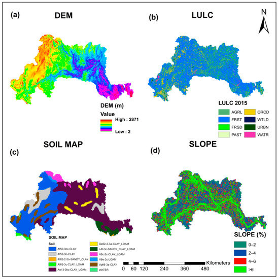
Figure 2.
(a) DEM; (b) LULC; (c) soil map; (d) slope of HRB.
2.2.2. GRACE (Gravity Recovery and Climate Experiment) Based TWSA
A novel method of remote sensed evapotranspiration (RSET) using (Gravity Recovery and Climate Experiment) GRACE processed data were forced into the SWAT model across the Hongshui River basin to anticipate hydrologic responses to future climatic conditions (HRB) and measured anomalies in the water mass stored. We computed the terrestrial water storage anomaly (TWSA) to assess the ET characteristics. We combined it with the water budget equation in the HRB based on GRACE with a spatial resolution of 0.50 degrees. Since the launch and implementation of the subsequent GRACE Follow-On (GRACE-FO) satellites, gravity satellites have been able to detect long-term hydrological change information at large scales, making them a useful tool for measuring regional land water storage changes on a global scale [78,79,80]. This dataset includes the GRACE/GRACE-FO RL06 Mascon data released by the Center for Space Research (CSR), real-time analysis system data of daily grid precipitation in China, CN05.1 temperature data, and other datasets. The Mascon outputs use a priori information resultant from near-global geophysical models to avoid stripping. Additionally, it is less susceptible to leakage errors than the harmonic solution (https://grace.jpl.nasa.gov/data/, accessed on 10 February 2023). In order to process the dataset, the scaling factor approach was applied, where each Mascon and the grid used to restore the lost signal had a resolution of 0.5°. After multiplying the Mascon grid by the scaling factor grid, all pixels within the study area with a resolution of 0.5° were spatially averaged over the study area to generate a time series. Additionally, the reason for using the GRACE ET data was to compare its estimates with those generated by SWAT, which can provide ET estimates and changes in storage. Our goal was to evaluate the suitability of the GRACE data as an input for hydrological modeling and compare it with the commonly used SWAT model.
2.3. Generalized Framework
The SWAT hydrological model combined with GRACE data was utilized to simulate the streamflow. SWAT is a gridded hydrological model with input data such as precipitation, wind speed, radiation, temperature, and reservoir operation data and combines the simulated baseflow and discharge to the routing model represented in Figure 3. For each grid cell upstream of the reservoir, it is essential to guide the runoff to the reservoir and then bias-correct the simulated streamflow using observed streamflow data collected before the reservoir’s construction. Furthermore, the study period was divided into two halves, a baseline period and a variation period, to study the change in the annual mean runoff. In addition to quantifying the hydrological sensitivity of climate change on streamflow using long-term water balance, this technique was utilized to measure the hydrological sensitivity of climate change.
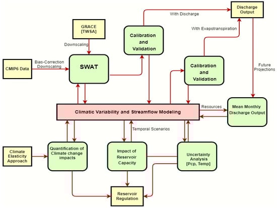
Figure 3.
Flowchart diagram of the generalized framework methodology.
2.4. Hydrological Modeling
SWAT is a physically-based, semi-distributed basin-scale model by Arnold et al. [81]. In addition to water balance and streamflow, the SWAT model can simulate hydrological processes such as lateral flow, snowmelt runoff, surface flow, and infiltration in a river basin using data on the daily and sub-daily precipitation, temperature, relative humidity, and wind speed [82,83,84]. The SWAT model assigns different classifications to different types of soil and vegetation based on the hydrologic response units of each (HRU). Runoff is calculated separately from HRUs, and the hydrological model determines how much runoff the entire watershed produces [62]. The equation below serves as the foundation for the SWAT hydrological model:
where is the ultimate amount of water in the soil; is the early water content in the soil; t is the number of days; is the daily precipitation; is the surface discharge; is the actual evapotranspiration; is the saturated water to the vadose zone; represents the sub-surface flow.
SUFI-2 was used to calibrate and validate the SWAT model, accounting for uncertainties in the driving variables, measurable datasets, and parameters [85]. The calibration (1991–1997) and validation (1998–2001) objective functions are shown below using the observed discharge data from the Qianjiang and Tiane hydrological stations, as illustrated in Figure 4. According to Table 4, the model’s performance indicators at Qianjiang station were better than at Tiane station. Throughout the calibration and validation processes, the model of each gauge station has iterated a total of one thousand times per month. To conduct a sensitivity analysis, SWAT-CUP used the Latin Hypercube and One-at-Time (LH-OAT) sampling technique. Table 5 presents the top 10 groups of model parameters identified as having a substantial impact on the results produced by the model and were therefore given the designation of sensitive parameters [86].
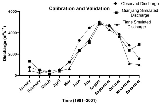
Figure 4.
Calibration and validation of the monthly observed and simulated discharge at the outlet of the HRB.
Table 4.
Objective functions indices of the monthly simulated and observed streamflow at Qianjiang and Tiane hydrological stations.
Table 5.
Group of sensitive parameters with the initial, final, fitted values, P-factor, and T-stat.
2.5. Objective Functions Indices
Using objective functions is necessary to validate the performance of the hydrological models. The statistical performance of the SWAT model was evaluated in this research using the Nash–Sutcliffe efficiency (NSE), the correlation coefficient (R2), and the percent bias (PBIAS), as shown in Table 3. R2 is the correlation between data that has been simulated and data that has been observed and may take on values between 0 and 1; with the performance increasing, the closer it is to 1. The following expression may be used to represent R2:
where and are the observed and simulated discharge, respectively.
A normalized dimensionless statistic called the Nash–Sutcliffe efficiency (NSE) illustrates how much residual variation there is compared to the observed data’s variance [87]. NSE can be calculated using the equation below:
where and are the observed and simulated discharge at the ith observation, respectively; is the mean observed discharge data over the simulation period. The NSE value is limited from −∞ to 1, with the best value of 1 [88].
The PBIAS (percent bias) formula determines the average deviation of the simulated values from the observed ones [88]. The model performance improves with less PBIAS. Here is an equation demonstrating the PBIAS:
where is the measured, is the simulated, and is the observed discharge at ith observation. PBIAS has an optimum value of zero; a positive PBIAS value implies a model underestimate, whereas negative values imply a model overestimation.
2.6. Climate Elasticity Approach (CEA)
Many researchers have used the idea of the climatic elasticity of streamflow as a theoretical framework [89,90]. It represents the runoff’s proportional reaction to changes in climatic component (in this case, ETP or precipitation). This can be spelled out as follows:
The water balance is governed by the available energy, atmospheric demand (ETP − ETo), and water availability, according to the Budyko hypothesis [91]. The ratio of annual evapotranspiration to precipitation (ET/P) is a function of the aridity index (φ = ETo/P) as derived from the Budyko hypothesis and the long-term water balance equation (Q = P − E), precipitation (εP), and potential evapotranspiration (εETo) [92]. Streamflow elasticity may be evaluated using the following:
Prior research studies presented several empirical equations for calculating F(φ). We used the Zhang et al. [93] and Fu [94] equations as their use and geographical characteristics were the same as ours. The F(φ) equation is given as follows:
The impact of climate change on the streamflow is then estimated as follows:
ΔP and ΔETo differ between the mean precipitation and evapotranspiration in the required and baseline periods. At the same time, P′ and ETo′ are the mean precipitation and evapotranspiration for the total period evaluated, respectively.
3. Results
3.1. Mean Climatology
3.1.1. Variance in Temperature Evolution
The scenarios accessible from most modeling centers are SSP1-2.6 (shared with RCP-2.6), SSP2-4.5, SSp3-7.0, and SSP5-8.5. Figure 5 depicts the progression of the average surface temperature (tas) of GCMs in the CMIP6 future scenarios. The difference was plotted with considerable changes projected in SSP1-2.6, while a significant change of 8 °C could be observed in SSP5-8.5. The temperature in SSP1-2.6 stayed constant throughout the 21st century, and the trend reaches its apex in the middle of the century before starting to decline toward the end. In contrast, the average temperatures will continue to climb until 2075 in SSP2-4.5, where the trends are sloped continuously. Temperature trends in SSP3-7.0 are similar to those in SPS2-4.5, despite exceeding 20 °C. The end of the 21st century will witness a significant climb to 22 °C and an increase in temperature anomalies in contrast to SPS5-8.5, where temperature trends have practically stabilized.
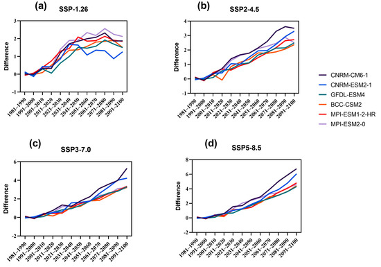
Figure 5.
Average surface temperature (tas) difference of GCMs members participating in CMIP6 over the Hongshui River basin (HRB).
In all four scenarios, CMIP6 had a stronger climate sensitivity and a larger trend in the average surface temperature (tas) compared to projections in CMIP5. This may partly explain the discrepancies in the projecting ability between CMIP5 and CMIP6 for the temperature variances and trends. A climate with an extended period and more disequilibrium has a larger positive temperature trend and higher sensitivity. Socio-economic pathway scenarios (SSPs) from six general circulation models (GCMs) imply different climatic changes across the Hongshui River basin (HRB). All GCMs projected temperature rises of 2 °C, although their monthly patterns varied. MRI-ESM2-0, GFDL-ESM-4, and CNRM-ESM2-1 GCMs demonstrated a steady temperature climate change signal for subbasins throughout the year while the BCC-CSM2 and MPI general circulation models showed minor changes.
3.1.2. Precipitation Patterns under Changing Climate
How well CMIP6 models replicate the climatological monthly precipitation and inter-annual variation throughout the whole HRB can be seen in Figure 6. The difference between the historical and future precipitation projections showed negative values in the first half of the 21st century. In contrast, the century’s second half will likely observe significant positive changes. There is a consistent pattern of rising mean monthly precipitation in the HRB from upstream to downstream. Sub-regional differences exist in the RBIAS that various CMIP6 models best suit. Multi-model ensemble mean (MEM) precipitation showed a 30% overestimation over the whole HRB (wet bias). The HRB RBIAS varied from 0.5% to 53.6% across all available models. The wet bias in the CMIP6 models was evident in all of the selected models and widespread over the HRB. In most CMIP6 models, significant relationships were seen between the annual projected precipitation and CMA data from 1970 to 2014. This suggests that most CMIP6 models for the HRB and sub-regions captured the natural variation in precipitation between years. Long-term changes in precipitation patterns throughout this time were also evaluated. In terms of characterizing the observed changing trends across the basin, GFDL-ESM4 was the best of the CMIP6 models; nonetheless, it missed the significance of a declining trend in the upstream channels of the basin. The average monthly rainfall (in mm) throughout the HRB, as projected by CMIP6 models, was analyzed seasonally. The relevant RBIAS from each CMIP6 model in the HRB was quantified to further characterize the seasonal biases of precipitation. Wet bias was undeniably an ever-present occurrence throughout all HRB seasons and geographies. The highest overestimation occurred in the cold season (spring and winter) and within specific HRB areas. A total of 13% in the spring (March–May), 15% in the summer (June–August), 12% in the fall (September–November), and 47% in the winter were seen in the HRB-wide RBIAS for MEM (December–February).
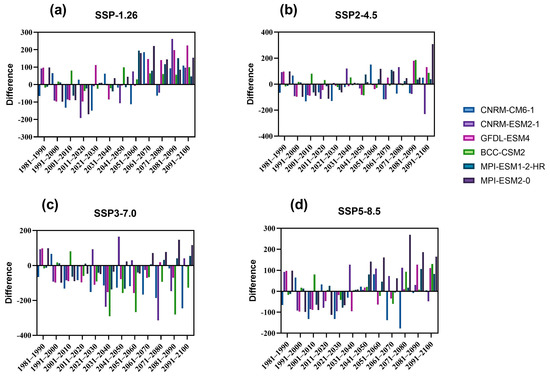
Figure 6.
Decade-wise time series plot of the difference in precipitation compared to the historically observed precipitation of GCM members from the CMIP6 outputs.
Figure 6 displays the CMIP6 member study, which indicated a significant decline in all four scenarios up to 2010, followed by an upward trend following that year. The peak in the SPS-2.6 scenario occurs in the early 2080s and is 4.7 mm/day. The decline is expected to persist until at least 2100. Until 2100, temperatures in the other three scenarios are also projected to increase by an average of 0.2 mm per day. The projections suggest that there will be significantly more precipitation than expected. Figure 7 shows that the downstream region of the basin is likely to receive more precipitation, followed by the central regions of the basin and the western parts. The least precipitation can be seen in the highest SSP585 scenario and the most in the lowest SSP-1.26 scenario, with peak values ranging from 56 mm/month to 71 mm/month. There was no consistency in the amount, direction, or seasonality of change, nor in the degree of similarity across sub-basins for the climate change signals associated with precipitation. In the whole Hongshui River basin (HRB), the BCC-CSM2 and MPI GCMs projected an increase in precipitation (by 5–16%), while the CNRM GCMs projected a reduction (by 1.5%).
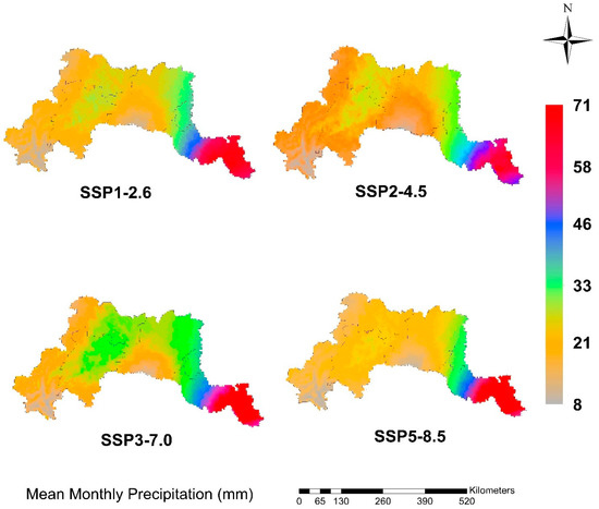
Figure 7.
Spatial distribution of the mean monthly precipitation (pr in mm) of the ensemble of GCM members over the Hongshui River basin (HRB).
3.2. Remote Sensing-Based Evapotranspiration (RSET)
Due to its importance in the water budget, evapotranspiration may be estimated using the terrestrial water balance equation’s residual: ETwb = P − Q − ds/dt, where P is the rainfall, Q is the discharging flow, and ds/dt represents changes in the water storage [95].
Validation of the GRACE ET data, as represented in Figure 8, allowed us to assess the accuracy and reliability of the data. This validation process involved comparing the GRACE ET data with the observed ET data and assessing the level of agreement between them. Through this validation process, we were able to better understand and account for the uncertainties associated with the GRACE ET data in our analysis. Due to the availability of remotely sensed data, the water balance method is often used to estimate ET at the basin scale and over months or even coarser periods. The ds/dt obtained only from the GRACE mission is depicted in Figure 9b. The ET data were evaluated for the six distinct zones described in Figure 9a,c represents the mean distribution of monthly ET data over six zones of study area. The drainage basin had an area of 98,500 km2. The area of the six zones varied from 10,000 km2 to 20,000 km2. These locations included the basin area and sites close to achieving more precise findings during the simulations. Because of the variations, the importance of ET in this region is particularly noteworthy.
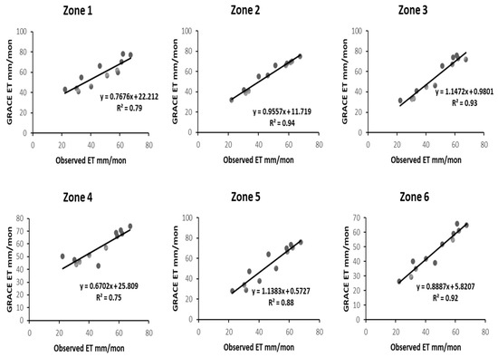
Figure 8.
Validation of the GRACE inferred ET data and observed ET dataset over the Hongshui River basin, China.
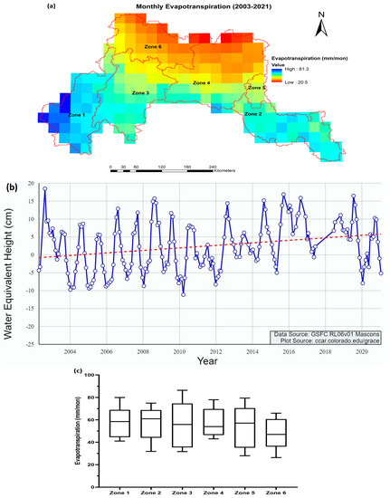
Figure 9.
(a) Mean monthly evapotranspiration data (ET) over Hongshui River basin (HRB). (b) GRACE (Gravity Recovery and Climate Experiment) data over HRB. Red dotted is a trend line over the time-period. (c) Mean monthly ET of six zones over HRB.
Based on the ET data, a simulation of the discharge was carried out. The mean monthly ET at different zones displayed in Figure 9c for 2003–2021 were assessed and varied from 20.5 mm/month to 81.3 mm/month.
Figure 10 depicts the link between the simulation discharge and evapotranspiration and the association between the simulation discharge and precipitation. The R2 and NSE statistical parameter indices offered satisfactory findings, with 0.78 and 0.80, respectively. The results extracted from Figure 10 showed that the peaks of the calibrated discharge were slightly greater than the peaks of calibration with ET. These larger peaks suggest that the data gathered by remote sensing for evapotranspiration were overestimated.
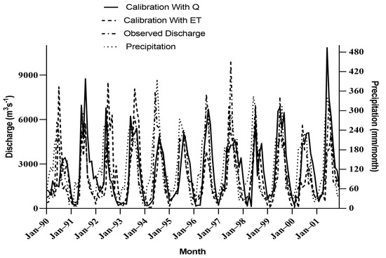
Figure 10.
Calibration and validation of the simulated discharge Q and evapotranspiration ET with the observed discharge and the correlation of precipitation and discharge over the Hongshui River basin (HRB).
3.3. Mean Monthly Projected Discharge (MMPD)
The variances in inter-GCMs are shown by the results obtained by running the model with ET data acquired from GRACE for six different GCMs. The impacts of the climate change and projections on streamflow in the Hongshui River basin (HRB) were analyzed. Figure 11 shows Sen’s estimates, a minimum and maximum confidence level of 99% and 95%, respectively, and the residual data from each of the four scenarios for the discharge simulation. The magnitude of the discharge is projected to decrease throughout the first five months of the year, followed by a minor increase throughout the summer. The GFDL-ESM4 model anticipated that there would be a negative change in each of the four scenarios. The findings of other models point to either an increasing trend or the lack of a significant shift in the link between the streamflow and precipitation. According to the average changes in long-term future scenarios, it is anticipated that the streamflow in the future will increase by 4.2% if the SSP-1.26 scenario plays out, 6.2% if the SSP-2.45 scenario plays out, 8.45% if the SSP-3.70 scenario plays out, and 9.5% if the SSP-5.85 scenario plays out.
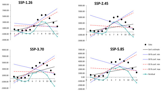
Figure 11.
Sen’s estimate, a minimum and maximum confidence level of 99% and 95%, and the residual data of the simulated mean monthly discharge (CMS) from each of the four scenarios.
Similarly, an analysis was conducted on how climate change influences streamflow seasonality. The impact will most likely be felt during the year’s colder months. Compared to the rainy season, May–September, the change in streamflow between January and April was significantly larger. The dry climate caused a reduction in streamflow. The precipitation trends throughout this time also contributed to the overall decrease, which showed its most pronounced effects between January and April. The most important factor that contributes to differences in discharge variance is precipitation. Near-surface air temperature and evapotranspiration are also important, although they only play a supporting role. As a result, there is a high degree of confidence that the streamflow will continue to drop as the near-surface air temperature rises over the 21st century. This will lead to a decrease in river basin discharge by the year 2100 under the climatic scenarios that are the hottest.
3.4. Climate Variability Contribution to Streamflow
The climatic elasticity method is used to calculate the relative contribution of climate change in determining streamflow. Table 6 displays εp and εETo for each of the different equations of F(φ) for HRB and the contribution of climate change to streamflow (ΔQc).
Table 6.
Climate change contribution (ΔQc) using the (CEM) climate elasticity method.
The contribution of climate change in the streamflow for the Hongshui River basin (HRB) was 10.8% and 12.5% as per Zhang, Dawes, and Walker [93] and Fu [94], respectively, which are indeed a contribution. This concludes that this basin will face other factors such as human-induced changes, deforestation, and water storage, contributing significantly to streamflow variability.
3.5. Impact Assessment of Reservoirs Capacity on Streamflow
The effect evaluation of reservoir capacity on streamflow in the Hongshui River basin was examined through the lens of four distinct scenarios. Table 1 contains information on the parameters of the reservoirs, while Figure 1 presents the data regarding the locations of the reservoirs. Scenario 1 is the standard, natural-based situation scenario that is a benchmark against which other scenarios may be assessed. Figure 12a shows the mean monthly discharge at the Qianjiang outlet; the other three scenarios are yearly, monthly, and daily regulatory reservoirs. The absolute difference between the mean monthly discharge with and without reservoirs divided by the monthly average flow without reservoirs yields a relative difference. From May through October, the MMD with the reservoir was only slightly higher than the natural monthly average flow, as shown in Figure 12b, with January and March seeing the greatest spike. In addition, increasing capacity resulted in more runoff throughout the dry season. The dry season significantly increased the monthly average flow to the yearly regulation reservoir. At the height of the flood season, from June to September, the annual regulatory reservoir effectively mitigated flood damage. The monthly and daily regulation reservoir induced a decrease in runoff in June and July, followed by a small increase in August and September.
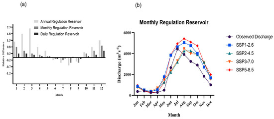
Figure 12.
(a) Annual, monthly, and daily regulation reservoirs on the MMD at the Qianjiang outlet station. (b) MMD regulation reservoir at the Longtan reservoir.
4. Discussion
The effects of global warming on weather phenomena such as rainfall, temperature, runoff tendencies, streamflow variability, discharge modeling using remotely sensed evapotranspiration, and reservoir capacity assessment were examined. For CMIP6, a brand-new set of SSP scenarios encompassing various probable socio-economic changes was created. The SSPs mirror many obstacles in the fight against and adaptation to climate change. For instance, the SSP5-8.5 scenario has the same radiative forcing as RCP 8.5 but projects greater globalization, the rapid economic and social growth of emerging nations, and the use of abundant fossil fuel resources. The SSP stories lead to increasingly high temperatures from SSP126, SSP245, and SSP370 through SSP585 [96,97]. We focused primarily on the twentieth century (1960–2020) and the twenty-first century (2021–2100) SSPs run for CMIP6. This research shows that the BCC-CSM2 and MPI GCMs suggest yearly rising precipitation (5–16%) for the whole Hongshui River basin (HRB). Similar to our results, other studies indicate that the annual mean precipitation in South Asia would rise by 8.7%, 11.6%, and 25.1% by the end of the twenty-first century under the three SSP scenarios, respectively. There are not a lot of variations in the yearly mean precipitation between adjacent nations. The precipitation is projected to likely increase the most under SSP5-8.5. Bangladesh will likely observe an increase of 4.4–17.1% in the annual mean rainfall [98], 1.6–18.9% for Bhutan, 6.6–21.2% for Sri Lanka [19], 9.3 to 27.3% for India [99], and precipitation in Pakistan is projected to rise by 9.3–26.4% as well as an increase of 3.6–19.5% over Nepal under shared socio-economic pathways [100]. Similar results have reported that future precipitation is projected to increase by 6.0% under RCP-2.6 and 12.0% under the RCP-8.5 scenario over the western highlands of China [101]. With minor differences in the expected magnitudes, the current findings are consistent with prior research [102,103].
Annual mean temperature projections over the HRB were evaluated, and an ensemble of GCMs showed a rise of nearly 2 °C; nonetheless, GCMs differ in how they project monthly temperature increases. The results correspond to other regional studies; the average temperature over South Asia is projected to increase by 0.8 °C, 0.9 °C, and 1.2 °C in the near future period; 1.2 °C, 1.8 °C, and 2.9 °C, throughout the mid-future period; 1.2 °C, 2.1 °C, and 4.3 °C for the far period under the low, medium, and high SSPs, respectively [19]. Neighboring country Nepal will likely observe an increase of 1.7–3.6 °C by 2100 [104].
Using satellite-based data to improve the model results is a possibility. In light of this objective, a framework is suggested to facilitate the application of remotely sensed observations to enhance hydrological modeling. This study used the SRTM-DEM, LULC 2015 by ESA, the global soil map by FAO, and remotely sensed evapotranspiration ET from the GRACE mission was utilized together in hydrological modeling, which was seldomly reported in early research [76,77,105]. Several researchers have benefited from GRACE estimates in various ways such as the water balance data, groundwater data, monitoring the decline in water resources, and enhancing the hydrological models [78,106]. The results of the models using remotely sensed soil moisture, ET, or streamflow measurements alone or in combination may be compared to improve the hydrological projections. As projected by the SWAT-based simulation, most models would experience either increasing tendencies or no noticeable changes in streamflow and precipitation. Long-term trends indicate that streamflow will increase by 4.2% in SSP-1.26, 6.2% in SSP-2.45, 8.45% in SSP-3.70, and 9.5% in SSP-5.85. There will be a rise in the summer and a fall in the winter. The results coincide with Lü-Liu et al. [107], where rising trends in the area averaged monthly precipitation and runoff have been projected from May to October.
In contrast, decreasing trends have been projected from December to February. In contrast, Zhang, Lu, Higgitt, Chen, Han, and Sun [67] found no significant trend or sudden change, and discharges were mostly controlled by precipitation variability. In contrast, reservoir/dam building in the Zhujiang basin had a minimal effect on water discharge. Several regional studies have found a downward trend in streamflow during the 1990s, most likely due to decreased precipitation [108,109].
The relative contribution of climate change in the streamflow using the climate elasticity technique is 10.8% and 12.5% for the Hongshui River Basin (HRB), as per Zhang et al. [110] and Fu [94], respectively, which is certainly a contribution. Assani et al. [111] found that the basin’s characteristics changed significantly as the number of reservoirs increased. This harms runoff generation within the basin and poses many challenges for future studies of the hydrological cycle. Moreover, Liu et al. [112] reported either no link or a modest correlation between the downstream flow from a reservoir and the climatic factors (precipitation and temperature).
The effect evaluation of reservoir capacity on streamflow from October to May indicates that the MMD with the reservoir is somewhat greater than the natural MMD, with the most significant increase happening between January and March. Runoff during the dry season will also grow considerably when the capacity is increased. At the yearly regulatory reservoir, the dry season saw the greatest rise in MMD. Similar studies have uncovered the downstream flooding consequences of hydropower station reservoir adjustments made for flood control throughout numerous typical years. Summer runoff is reduced by 10% to 50%, and winter runoff is reduced by 45% to 85% due to the functioning of two huge reservoirs in the upstream region of the Yenisei River [113].
Limitation and Future Considerations
The contributions of our study should be seen in light of the following limitations, which can be addressed by future investigations to further improve the streamflow modeling and forecasting of hydrological parameters. First, although the current resolution (~50 km) of the GRACE estimates has paved a way of deriving helpful information regarding hydrological simulation, its coarse resolution holds back its feasibility for local/regional scale monitoring [114]. Therefore, hydrological measurements are necessary at a higher resolution to have better and more precise projections, for example, increasing the spatial resolution with machine learning algorithms [51,115], random forest (RF) algorithm [44], and deep learning (DL) [116,117]. The current proposed combined approach of pre-processed GRACE data with SWAT indicates a high correlation of coefficient (R) and NSE values. After improving the resolution of GRACE data at a spatial scale based on the above-mentioned downscaling methods, it competently allows for the evaluation of TWS in more detail at a small regional scale worldwide.
Second, the validation analysis part is constrained due to data scarcity. This study validated ET-GRACE derived based on the water balance equation with the observed ET data and it performed well, but there were still several uncertainty sources involved in this study. The precipitation “P” and runoff data “Q” ultimately accounted for the ET estimation. Therefore, to minimize the uncertainties, we proposed the validation of the individual parameters “P” and “Q” to recognize the relative uncertainties in GRACE and other water balance fluxes [59]. Finally, this study used input data such as the LULC, DEM, and soil map for hydrological simulation, and proposed the latest version of the input data and a finer resolution for more accurate projections. Future research should ideally include a more comprehensive accounting of the parameters governing the surface and subsurface flow in this and other heterogeneous systems.
5. Conclusions
A novel approach for simulating discharge in the SWAT model was suggested in this paper. Incorporating remotely sensed evapotranspiration pre-processed GRACE data, precipitation, and temperature data derived from CMIP6-developed SSPs and reservoir data improved the accuracy of the hydrological models. In addition, the impact of changing climate on precipitation, temperature, runoff trends, streamflow variability, discharge modeling based on remotely sensed evapotranspiration, and reservoir capacity assessment were investigated. The following conclusions were summarized. (a) The analysis of SSPs run for CMIP6 models for the second half of the twentieth century (1960–2020 of historical run) and twenty-first century (2021–2100) concluded that the BCC-CSM2 and MPI GCMs showed increasing annual precipitation (by 5–16%) for the entire Hongshui River basin (HRB). (b) The anticipated increases in the annual mean temperature throughout the entire HRB were examined, and an ensemble of GCMs showed an increase of nearly 2 °C. (c) The scenarios suggest that the future streamflow will rise by 4.2% under SSP-1.26, 6.2% under SSP-2.45, 8.45% under SSP-3.70, and 9.5% under SSP-5.85. Summer will likely observe an increase, while winter will see a decline. (d) Using the climate elasticity technique, the relative contribution of climate change in the streamflow for the Hongshui River basin (HRB) is 10.8% and 12.5%. (e) The monthly and daily regulation reservoir reduces runoff from June to July while increasing somewhat from August to September. The use of satellite-based observations may aid in improving the model findings. In light of this goal, a framework is provided to aid in using remotely sensed data to improve basin-scale hydrological models. There is a lot of room for error when trying to project hydrological variables. Still, the results from most modeling ensemble members are good enough to be utilized as a basis for water resource management in the future. In general, reservoir operation may delay the onset of floods and lessen their severity, and it can release more water during the dry season to meet the downstream water demands.
Author Contributions
M.T. devised the idea, performed the analysis, designed the study, and wrote the paper. L.C. and H.C. provided the technical support and supervision. W.Y. provided the required data while H.F.G. and A.M. revised the manuscript for corrections and proofreading. All authors have read and agreed to the published version of the manuscript.
Funding
This study was supported by the National Natural Science Foundation of China [52069002, 51669003], the Major Science and Technology Projects of the Ministry of Water Resources of China [SKR-2022038], the Scientific Research and Technology development Program of Nanning City [20223054] and the Innovation Project of Guangxi Graduate Education [YCBZ2023002].
Data Availability Statement
Primary datasets are available upon request.
Acknowledgments
The authors would like to thank the National Meteorological Information Centre (NMIC) of the China Meteorological Administration (CMA) for the great help and support in the data exchange.
Conflicts of Interest
The authors declare no conflict of interest.
References
- Scanlon, B.R.; Jolly, I.D.; Sophocleous, M.; Zhang, L. Global impacts of agricultural land-use changes on water resources: Quantity versus quality. Water Resour. Res. 2006, 43, 3. [Google Scholar] [CrossRef]
- Ahmadaali, J.; Barani, G.-A.; Qaderi, K.; Hessari, B. Analysis of the Effects of Water Management Strategies and Climate Change on the Environmental and Agricultural Sustainability of Urmia Lake Basin, Iran. Water 2018, 10, 160. [Google Scholar] [CrossRef]
- Chen, Y.; Takeuchi, K.; Xu, C.; Chen, Y.; Xu, Z. Regional climate change and its effects on river runoff in the Tarim Basin, China. Hydrol. Process. 2006, 20, 2207–2216. [Google Scholar] [CrossRef]
- Kiparsky, M.; Joyce, B.; Purkey, D.; Young, C. Potential impacts of climate warming on water supply reliability in the Tuolumne and Merced river basins, California. PLoS ONE 2014, 9, e84946. [Google Scholar] [CrossRef] [PubMed]
- Han, Z.; Long, D.; Fang, Y.; Hou, A.; Hong, Y. Impacts of climate change and human activities on the flow regime of the dammed Lancang River in Southwest China. J. Hydrol. 2019, 570, 96–105. [Google Scholar] [CrossRef]
- Chang, J.; Wang, Y.; Istanbulluoglu, E.; Bai, T.; Huang, Q.; Yang, D.; Huang, S. Impact of climate change and human activities on runoff in the Weihe River Basin, China. Quat. Int. 2015, 380, 169–179. [Google Scholar] [CrossRef]
- Gao, P.; Geissen, V.; Ritsema, C.; Mu, X.-M.; Wang, F. Impact of climate change and anthropogenic activities on stream flow and sediment discharge in the Wei River basin, China. Hydrol. Earth Syst. Sci. 2013, 17, 961. [Google Scholar] [CrossRef]
- Zuo, D.; Xu, Z.; Wu, W.; Zhao, J.; Zhao, F. Identification of streamflow response to climate change and human activities in the Wei River Basin, China. Water Resour. Manag. 2014, 28, 833–851. [Google Scholar] [CrossRef]
- Wang, S.; Yan, M.; Yan, Y.; Shi, C.; He, L. Contributions of climate change and human activities to the changes in runoff increment in different sections of the Yellow River. Quat. Int. 2012, 282, 66–77. [Google Scholar] [CrossRef]
- Zhao, G.; Tian, P.; Mu, X.; Jiao, J.; Wang, F.; Gao, P. Quantifying the impact of climate variability and human activities on streamflow in the middle reaches of the Yellow River basin, China. J. Hydrol. 2014, 519, 387–398. [Google Scholar] [CrossRef]
- Huang, Y.; Wang, H.; Xiao, W.H.; Chen, L.H.; Zhou, Y.Y.; Song, X.Y.; Wang, H.J. Contributions of climate change and anthropogenic activities to runoff change in the Hongshui River, Southwest China. IOP Conf. Ser. Earth Environ. Sci. 2018, 191, 012143. [Google Scholar] [CrossRef]
- Adib, M.N.M.; Harun, S. Metalearning Approach Coupled with CMIP6 Multi-GCM for Future Monthly Streamflow Forecasting. J. Hydrol. Eng. 2022, 27, 05022004. [Google Scholar] [CrossRef]
- Xiang, Y.; Wang, Y.; Chen, Y.; Zhang, Q. Impact of Climate Change on the Hydrological Regime of the Yarkant River Basin, China: An Assessment Using Three SSP Scenarios of CMIP6 GCMs. Remote Sens. 2022, 14, 115. [Google Scholar] [CrossRef]
- Konapala, G.; Mishra, A.K.; Wada, Y.; Mann, M.E. Climate change will affect global water availability through compounding changes in seasonal precipitation and evaporation. Nat. Commun. 2020, 11, 3044. [Google Scholar] [CrossRef]
- Chen, Y.; Liu, A.; Zhang, Z.; Hope, C.; Crabbe, M.J.C. Economic losses of carbon emissions from circum-Arctic permafrost regions under RCP-SSP scenarios. Sci. Total Environ. 2019, 658, 1064–1068. [Google Scholar] [CrossRef]
- Moss, R.H.; Edmonds, J.A.; Hibbard, K.A.; Manning, M.R.; Rose, S.K.; Van Vuuren, D.P.; Carter, T.R.; Emori, S.; Kainuma, M.; Kram, T.J.N. The next generation of scenarios for climate change research and assessment. Nature 2010, 463, 747–756. [Google Scholar] [CrossRef]
- Li, S.-Y.; Miao, L.-J.; Jiang, Z.-H.; Wang, G.-J.; Gnyawali, K.R.; Zhang, J.; Zhang, H.; Fang, K.; He, Y.; Li, C. Projected drought conditions in Northwest China with CMIP6 models under combined SSPs and RCPs for 2015–2099. Adv. Clim. Change Res. 2020, 11, 210–217. [Google Scholar] [CrossRef]
- Almazroui, M.; Saeed, F.; Saeed, S.; Nazrul Islam, M.; Ismail, M.; Klutse, N.A.B.; Siddiqui, M.H. Projected change in temperature and precipitation over Africa from CMIP6. Earth Syst. Environ. 2020, 4, 455–475. [Google Scholar] [CrossRef]
- Almazroui, M.; Saeed, S.; Saeed, F.; Islam, M.N.; Ismail, M. Projections of Precipitation and Temperature over the South Asian Countries in CMIP6. Earth Syst. Environ. 2020, 4, 297–320. [Google Scholar] [CrossRef]
- O’Neill, B.C.; Kriegler, E.; Riahi, K.; Ebi, K.L.; Hallegatte, S.; Carter, T.R.; Mathur, R.; van Vuuren, D.P. A new scenario framework for climate change research: The concept of shared socioeconomic pathways. Clim. Change 2014, 122, 387–400. [Google Scholar] [CrossRef]
- Grose, M.R.; Gregory, J.; Colman, R.; Andrews, T. What Climate Sensitivity Index Is Most Useful for Projections? Geophys. Res. Lett. 2018, 45, 1559–1566. [Google Scholar] [CrossRef]
- Van Vuuren, D.P.; Edmonds, J.; Kainuma, M.; Riahi, K.; Thomson, A.; Hibbard, K.; Hurtt, G.C.; Kram, T.; Krey, V.; Lamarque, J.-F. The representative concentration pathways: An overview. Clim. Change 2011, 109, 5–31. [Google Scholar] [CrossRef]
- Fenicia, F.; Savenije, H.H.G.; Matgen, P.; Pfister, L. A comparison of alternative multiobjective calibration strategies for hydrological modeling. Water Resour. Res. 2007, 43, 3. [Google Scholar] [CrossRef]
- Molina-Navarro, E.; Andersen, H.E.; Nielsen, A.; Thodsen, H.; Trolle, D. The impact of the objective function in multi-site and multi-variable calibration of the SWAT model. Environ. Model. Softw. 2017, 93, 255–267. [Google Scholar] [CrossRef]
- Immerzeel, W.W.; Droogers, P. Calibration of a distributed hydrological model based on satellite evapotranspiration. J. Hydrol. 2008, 349, 411–424. [Google Scholar] [CrossRef]
- Rientjes, T.H.M.; Muthuwatta, L.P.; Bos, M.G.; Booij, M.J.; Bhatti, H.A. Multi-variable calibration of a semi-distributed hydrological model using streamflow data and satellite-based evapotranspiration. J. Hydrol. 2013, 505, 276–290. [Google Scholar] [CrossRef]
- Franco, A.C.L.; Bonumá, N.B.J.R. Multi-variable SWAT model calibration with remotely sensed evapotranspiration and observed flow. Braz. J. Water Resour. 2017, 22. [Google Scholar] [CrossRef]
- Githui, F.; Selle, B.; Thayalakumaran, T. Recharge estimation using remotely sensed evapotranspiration in an irrigated catchment in southeast Australia. Hydrol. Process. 2012, 26, 1379–1389. [Google Scholar] [CrossRef]
- Poortinga, A.; Bastiaanssen, W.; Simons, G.; Saah, D.; Senay, G.; Fenn, M.; Bean, B.; Kadyszewski, J. A Self-Calibrating Runoff and Streamflow Remote Sensing Model for Ungauged Basins Using Open-Access Earth Observation Data. Remote Sens. 2017, 9, 86. [Google Scholar] [CrossRef]
- Jiang, D.; Wang, K. The Role of Satellite-Based Remote Sensing in Improving Simulated Streamflow: A Review. Remote Sens. 2019, 11, 1615. [Google Scholar] [CrossRef]
- Finger, D.; Pellicciotti, F.; Konz, M.; Rimkus, S.; Burlando, P. The value of glacier mass balance, satellite snow cover images, and hourly discharge for improving the performance of a physically based distributed hydrological model. Water Resour. Res. 2011, 47, 7. [Google Scholar] [CrossRef]
- Finger, D.; Vis, M.; Huss, M.; Seibert, J. The value of multiple data set calibration versus model complexity for improving the performance of hydrological models in mountain catchments. Water Resour. Res. 2015, 51, 1939–1958. [Google Scholar] [CrossRef]
- Campo, L.; Caparrini, F.; Castelli, F. Use of multi-platform, multi-temporal remote-sensing data for calibration of a distributed hydrological model: An application in the Arno basin, Italy. Hydrol. Process. Int. J. 2006, 20, 2693–2712. [Google Scholar] [CrossRef]
- Li, Y.; Grimaldi, S.; Pauwels, V.R.; Walker, J.P. Hydrologic model calibration using remotely sensed soil moisture and discharge measurements: The impact on predictions at gauged and ungauged locations. J. Hydrol. 2018, 557, 897–909. [Google Scholar] [CrossRef]
- Kunnath-Poovakka, A.; Ryu, D.; Renzullo, L.J.; George, B. The efficacy of calibrating hydrologic model using remotely sensed evapotranspiration and soil moisture for streamflow prediction. J. Hydrol. 2016, 535, 509–524. [Google Scholar] [CrossRef]
- Corbari, C.; Mancini, M. Calibration and validation of a distributed energy–water balance model using satellite data of land surface temperature and ground discharge measurements. J. Hydrometeorol. 2014, 15, 376–392. [Google Scholar] [CrossRef]
- Sirisena, T.A.J.G.; Maskey, S.; Ranasinghe, R. Hydrological Model Calibration with Streamflow and Remote Sensing Based Evapotranspiration Data in a Data Poor Basin. Remote Sens. 2020, 12, 3768. [Google Scholar] [CrossRef]
- Winsemius, H.C.; Schaefli, B.; Montanari, A.; Savenije, H.H.G. On the calibration of hydrological models in ungauged basins: A framework for integrating hard and soft hydrological information. Water Resour. Res. 2009, 45, 12. [Google Scholar] [CrossRef]
- Tobin, K.J.; Bennett, M.E. Constraining SWAT Calibration with Remotely Sensed Evapotranspiration Data. J. Am. Water Resour. Assoc. 2017, 53, 593–604. [Google Scholar] [CrossRef]
- Pan, S.; Liu, L.; Bai, Z.; Xu, Y.-P. Integration of Remote Sensing Evapotranspiration into Multi-Objective Calibration of Distributed Hydrology–Soil–Vegetation Model (DHSVM) in a Humid Region of China. Water 2018, 10, 1841. [Google Scholar] [CrossRef]
- López López, P.; Sutanudjaja, E.H.; Schellekens, J.; Sterk, G.; Bierkens, M.F.J.H.; Sciences, E.S. Calibration of a large-scale hydrological model using satellite-based soil moisture and evapotranspiration products. Hydrol. Earth Syst. Sci. 2017, 21, 3125–3144. [Google Scholar] [CrossRef]
- Zhang, K.; Kimball, J.S.; Running, S.W. A review of remote sensing based actual evapotranspiration estimation. Wiley Interdiscip. Rev. Water 2016, 3, 834–853. [Google Scholar] [CrossRef]
- Long, D.; Longuevergne, L.; Scanlon, B.R. Uncertainty in evapotranspiration from land surface modeling, remote sensing, and GRACE satellites. Water Resour. Res. 2014, 50, 1131–1151. [Google Scholar] [CrossRef]
- Chen, L.; He, Q.; Liu, K.; Li, J.; Jing, C. Downscaling of GRACE-Derived Groundwater Storage Based on the Random Forest Model. Remote Sens. 2019, 11, 2979. [Google Scholar] [CrossRef]
- Long, D.; Yang, Y.; Wada, Y.; Hong, Y.; Liang, W.; Chen, Y.; Yong, B.; Hou, A.; Wei, J.; Chen, L. Deriving scaling factors using a global hydrological model to restore GRACE total water storage changes for China’s Yangtze River Basin. Remote Sens. Environ. 2015, 168, 177–193. [Google Scholar] [CrossRef]
- Rodell, M.; Famiglietti, J.; Wiese, D.; Reager, J.; Beaudoing, H.; Landerer, F. Emerging trends in global freshwater availability. Nature 2018, 557, 651–659. [Google Scholar] [CrossRef]
- Swenson, S.; Wahr, J.; Milly, P. Estimated accuracies of regional water storage variations inferred from the Gravity Recovery and Climate Experiment (GRACE). Water Resour. Res. 2003, 39, 8. [Google Scholar] [CrossRef]
- Richey, A.S.; Thomas, B.F.; Lo, M.H.; Reager, J.T.; Famiglietti, J.S.; Voss, K.; Swenson, S.; Rodell, M. Quantifying renewable groundwater stress with GRACE. Water Resour. Res. 2015, 51, 5217–5238. [Google Scholar] [CrossRef]
- Liu, Y.; Guo, W.; Feng, J.; Zhang, K. A Summary of Methods for Statistical Downscaling of Meteorological Data. Adv. Earth Sci. 2011, 26, 837. [Google Scholar]
- Lo, M.H.; Famiglietti, J.S.; Yeh, P.F.; Syed, T. Improving parameter estimation and water table depth simulation in a land surface model using GRACE water storage and estimated base flow data. Water Resour. Res. 2010, 46, 5. [Google Scholar] [CrossRef]
- Milewski, A.M.; Thomas, M.B.; Seyoum, W.M.; Rasmussen, T.C. Spatial Downscaling of GRACE TWSA Data to Identify Spatiotemporal Groundwater Level Trends in the Upper Floridan Aquifer, Georgia, USA. Remote Sens. 2019, 11, 2756. [Google Scholar] [CrossRef]
- Vishwakarma, B.D.; Zhang, J.; Sneeuw, N. Downscaling GRACE total water storage change using partial least squares regression. Sci. Data 2021, 8, 95. [Google Scholar] [CrossRef] [PubMed]
- Ali, S.; Khorrami, B.; Jehanzaib, M.; Tariq, A.; Ajmal, M.; Arshad, A.; Shafeeque, M.; Dilawar, A.; Basit, I.; Zhang, L.; et al. Spatial Downscaling of GRACE Data Based on XGBoost Model for Improved Understanding of Hydrological Droughts in the Indus Basin Irrigation System (IBIS). Remote Sens. 2023, 15, 873. [Google Scholar] [CrossRef]
- Yang, P.; Xia, J.; Zhan, C.; Wang, T. Reconstruction of terrestrial water storage anomalies in Northwest China during 1948–2002 using GRACE and GLDAS products. Hydrol. Res. 2018, 49, 1594–1607. [Google Scholar] [CrossRef]
- Breiman, L. Random forests. Mach. Learn. 2001, 45, 5–32. [Google Scholar] [CrossRef]
- Wang, J.; Zhang, J.; Ning, S.; Wang, H. Downscaling analysis of GRACE terrestrial water storage changes in Yunnan province. Water Resour. Power 2018, 336, 1–5. [Google Scholar]
- Vapnik, V. The Nature of Statistical Learning Theory; Springer Science & Business Media: Berlin, Germany, 1999. [Google Scholar]
- Ghorbani, M.A.; Khatibi, R.; Hosseini, B.; Bilgili, M. Relative importance of parameters affecting wind speed prediction using artificial neural networks. Theor. Appl. Climatol. 2013, 114, 107–114. [Google Scholar] [CrossRef]
- Arshad, A.; Mirchi, A.; Samimi, M.; Ahmad, B. Combining downscaled-GRACE data with SWAT to improve the estimation of groundwater storage and depletion variations in the Irrigated Indus Basin (IIB). Sci. Total Environ. 2022, 838, 156044. [Google Scholar] [CrossRef]
- Baldwin, C.K.; Lall, U. Seasonality of streamflow: The Upper Mississippi River. Water Resour. Res. 1999, 35, 1143–1154. [Google Scholar] [CrossRef]
- Song, W.-z.; Jiang, Y.-z.; Lei, X.-h.; Wang, H.; Shu, D.-c. Annual runoff and flood regime trend analysis and the relation with reservoirs in the Sanchahe River Basin, China. Quat. Int. 2015, 380–381, 197–206. [Google Scholar] [CrossRef]
- Guo, H.; Hu, Q.; Jiang, T. Annual and seasonal streamflow responses to climate and land-cover changes in the Poyang Lake basin, China. J. Hydrol. 2008, 355, 106–122. [Google Scholar] [CrossRef]
- Jia, L.; Li, Z.; Xu, G.; Ren, Z.; Li, P.; Cheng, Y.; Zhang, Y.; Wang, B.; Zhang, J.; Yu, S. Dynamic change of vegetation and its response to climate and topographic factors in the Xijiang River basin, China. Environ. Sci. Pollut. Res. 2020, 27, 11637–11648. [Google Scholar] [CrossRef] [PubMed]
- Lin, W.; Zhang, L.; Du, D.; Yang, L.; Lin, H.; Zhang, Y.; Li, J. Quantification of land use/land cover changes in Pearl River Delta and its impact on regional climate in summer using numerical modeling. Reg. Environ. Change 2009, 9, 75–82. [Google Scholar] [CrossRef]
- Seto, K.C.; Woodcock, C.; Song, C.; Huang, X.; Lu, J.; Kaufmann, R. Monitoring land-use change in the Pearl River Delta using Landsat TM. Int. J. Remote Sens. 2002, 23, 1985–2004. [Google Scholar] [CrossRef]
- Huang, Y.; Wang, H.; Xiao, W.; Chen, L.; Yan, D.; Zhou, Y.; Jiang, D.; Yang, M. Spatial and Temporal Variability in the Precipitation Concentration in the Upper Reaches of the Hongshui River Basin, Southwestern China. Adv. Meteorol. 2018, 2018, 4329757. [Google Scholar] [CrossRef]
- Zhang, S.; Lu, X.X.; Higgitt, D.L.; Chen, C.-T.A.; Han, J.; Sun, H. Recent changes of water discharge and sediment load in the Zhujiang (Pearl River) Basin, China. Glob. Planet. Change 2008, 60, 365–380. [Google Scholar] [CrossRef]
- Fischer, T.; Gemmer, M.; Su, B.; Scholten, T. Hydrological long-term dry and wet periods in the Xijiang River basin, South China. Hydrol. Earth Syst. Sci. 2013, 17, 135–148. [Google Scholar] [CrossRef]
- Touseef, M.; Chen, L.; Yang, K.; Chen, Y. Long-Term Rainfall Trends and Future Projections over Xijiang River Basin, China. Adv. Meteorol. 2020, 2020, 6852148. [Google Scholar] [CrossRef]
- Githui, F.; Gitau, W.; Mutua, F.; Bauwens, W. Climate change impact on SWAT simulated streamflow in western Kenya. Int. J. Climatol. A J. R. Meteorol. Soc. 2009, 29, 1823–1834. [Google Scholar] [CrossRef]
- Chen, Y.; Li, X.; Huang, K.; Luo, M.; Gao, M. High-resolution gridded population projections for China under the shared socioeconomic pathways. Earth’s Future 2020, 8, e2020EF001491. [Google Scholar] [CrossRef]
- O’neill, B.; Tebaldi, C.; Van Vuuren, D.; Eyring, V.; Friedlingstein, P.; Hurtt, G.; Knutti, R.; Kriegler, E.; Lamarque, J.; Lowe, J. The Scenario Model Intercomparison Project (ScenarioMIP) for CMIP6, Geosci. Model Dev. 2016, 9, 3461–3482. [Google Scholar] [CrossRef]
- Vaghefi, S.A.; Abbaspour, K. Climate Change Toolkit (CCT) User Guide. 2019. Available online: http://www.2w2e.com/home/CCT (accessed on 12 September 2022).
- Vaghefi, S.A.; Keykhai, M.; Jahanbakhshi, F.; Sheikholeslami, J.; Ahmadi, A.; Yang, H.; Abbaspour, K. The future of extreme climate in Iran. Sci. Rep. 2019, 1464, 2045–2322. [Google Scholar] [CrossRef] [PubMed]
- Abbaspour, K.C.; Faramarzi, M.; Ghasemi, S.S.; Yang, H. Assessing the impact of climate change on water resources in Iran. Water Resour. Res. 2009, 45, 10. [Google Scholar] [CrossRef]
- (CGIAR-CSI), C. Shuttle Radar Topography Mission Digital Elevation Model (SRTM-DEM). Available online: http://srtm.csi.cgiar.org/ (accessed on 12 July 2020).
- FAO. Food and Agriculture Organization (FAO). Available online: http://www.fao.org/nr/land/soils/digital-soil-map-of-the-world/en/ (accessed on 12 July 2020).
- Tapley, B.D.; Watkins, M.M.; Flechtner, F.; Reigber, C.; Bettadpur, S.; Rodell, M.; Sasgen, I.; Famiglietti, J.S.; Landerer, F.W.; Chambers, D.P. Contributions of GRACE to understanding climate change. Nat. Clim. Change 2019, 9, 358–369. [Google Scholar] [CrossRef] [PubMed]
- Feng, W.; Shum, C.K.; Zhong, M.; Pan, Y. Groundwater Storage Changes in China from Satellite Gravity: An Overview. Remote Sens. 2018, 10, 674. [Google Scholar] [CrossRef]
- Zhong, Y.; Feng, W.; Humphrey, V.; Zhong, M. Human-Induced and Climate-Driven Contributions to Water Storage Variations in the Haihe River Basin, China. Remote Sens. 2019, 11, 3050. [Google Scholar] [CrossRef]
- Arnold, J.G.; Moriasi, D.N.; Gassman, P.W.; Abbaspour, K.C.; White, M.J.; Srinivasan, R.; Santhi, C.; Harmel, R.; Van Griensven, A.; Van Liew, M.W. SWAT: Model use, calibration, and validation. J Trans. ASABE 2012, 55, 1491–1508. [Google Scholar] [CrossRef]
- Rostamian, R.; Jaleh, A.; Afyuni, M.; Mousavi, S.F.; Heidarpour, M.; Jalalian, A.; Abbaspour, K.C. Application of a SWAT model for estimating runoff and sediment in two mountainous basins in central Iran. Hydrol. Sci. J. 2010, 53, 977–988. [Google Scholar] [CrossRef]
- Wang, Y.J.; Meng, X.Y.; Liu, Z.H.; Ji, X.N. Snowmelt Runoff Analysis under Generated Climate Change Scenarios for the Juntanghu River Basin, in Xinjiang, China. Tecnol. Cienc. Agua 2016, 7, 41–54. [Google Scholar]
- Dhami, B.; Himanshu, S.K.; Pandey, A.; Gautam, A.K. Evaluation of the SWAT model for water balance study of a mountainous snowfed river basin of Nepal. Env. Earth Sci. 2018, 77, 21. [Google Scholar] [CrossRef]
- Abbaspour, K.C.; Rouholahnejad, E.; Vaghefi, S.; Srinivasan, R.; Yang, H.; Kløve, B. A continental-scale hydrology and water quality model for Europe: Calibration and uncertainty of a high-resolution large-scale SWAT model. J. Hydrol. 2015, 524, 733–752. [Google Scholar] [CrossRef]
- Vetter, T.; Reinhardt, J.; Flörke, M.; van Griensven, A.; Hattermann, F.; Huang, S.; Koch, H.; Pechlivanidis, I.G.; Plötner, S.; Seidou, O.; et al. Evaluation of sources of uncertainty in projected hydrological changes under climate change in 12 large-scale river basins. Clim. Change 2017, 141, 419–433. [Google Scholar] [CrossRef]
- Nash, J.E.; Sutcliffe, J.V. River flow forecasting through conceptual models part I—A discussion of principles. J. Hydrol. 1970, 10, 282–290. [Google Scholar] [CrossRef]
- Gupta, H.V.; Sorooshian, S.; Yapo, P.O. Status of automatic calibration for hydrologic models: Comparison with multilevel expert calibration. J. Hydrol. Eng. 1999, 4, 135–143. [Google Scholar] [CrossRef]
- Schaake, J.C.; Waggoner, P. From Climate to Flow; John Wiley and Sons Inc.: New York, NY, USA, 1990. [Google Scholar]
- De Freitas, G.N. São Paulo drought: Trends in streamflow and their relationship to climate and human-induced change in Cantareira watershed, Southeast Brazil. Hydrol. Res. 2020, 51, 750–767. [Google Scholar] [CrossRef]
- Budyko, M.I. Evaporation under Natural Conditions. 1963. Available online: http://agris.fao.org/agris-search/search.do?recordID=US201300573953 (accessed on 20 November 2022).
- Arora, V.K. The use of the aridity index to assess climate change effect on annual runoff. J. Hydrol. 2002, 265, 164–177. [Google Scholar] [CrossRef]
- Zhang, L.; Dawes, W.; Walker, G. Response of mean annual evapotranspiration to vegetation changes at catchment scale. Water Resour. Res. 2001, 37, 701–708. [Google Scholar] [CrossRef]
- Fu, B. On the calculation of the evaporation from land surface. Sci. Atmos. Sin 1981, 5, 23–31. [Google Scholar]
- Khorrami, B.; Gorjifard, S.; Ali, S.; Feizizadeh, B. Local-scale monitoring of evapotranspiration based on downscaled GRACE observations and remotely sensed data: An application of terrestrial water balance approach. Earth Sci. Inform. 2023, 1–17. [Google Scholar] [CrossRef]
- O’Neill, B.C.; Kriegler, E.; Ebi, K.L.; Kemp-Benedict, E.; Riahi, K.; Rothman, D.S.; van Ruijven, B.J.; van Vuuren, D.P.; Birkmann, J.; Kok, K. The roads ahead: Narratives for shared socioeconomic pathways describing world futures in the 21st century. Glob. Environ. Change 2017, 42, 169–180. [Google Scholar] [CrossRef]
- Yun, K.-S.; Lee, J.-Y.; Timmermann, A.; Stein, K.; Stuecker, M.F.; Fyfe, J.C.; Chung, E.-S. Increasing ENSO–rainfall variability due to changes in future tropical temperature–rainfall relationship. Commun. Earth Environ. 2021, 2, 43. [Google Scholar] [CrossRef]
- Caesar, J.; Janes, T.; Lindsay, A.; Bhaskaran, B. Temperature and precipitation projections over Bangladesh and the upstream Ganges, Brahmaputra and Meghna systems. Environ. Sci. Process. Impacts 2015, 17, 1047–1056. [Google Scholar] [CrossRef] [PubMed]
- Chhetri, R.; Pandey, V.P.; Talchabhadel, R.; Thapa, B.R. How do CMIP6 models project changes in precipitation extremes over seasons and locations across the mid hills of Nepal? Theor. Appl. Climatol. 2021, 145, 1127–1144. [Google Scholar] [CrossRef]
- Islam, M.; Das, S.; Uyeda, H. Calibration of TRMM derived rainfall over Nepal during 1998-2007. Open Atmos. Sci. J. 2010, 14, 2020. [Google Scholar] [CrossRef]
- Chong-Hai, X.; Ying, X. The Projection of Temperature and Precipitation over China under RCP Scenarios using a CMIP5 Multi-Model Ensemble. Atmos. Ocean. Sci. Lett. 2012, 5, 527–533. [Google Scholar] [CrossRef]
- Chanapathi, T.; Thatikonda, S.; Raghavan, S. Analysis of rainfall extremes and water yield of Krishna river basin under future climate scenarios. J. Hydrol. Reg. Stud. 2018, 19, 287–306. [Google Scholar] [CrossRef]
- Goswami, B.N.; Madhusoodanan, M.; Neema, C.; Sengupta, D. A physical mechanism for North Atlantic SST influence on the Indian summer monsoon. Geophys. Res. Lett. 2006, 33, 2. [Google Scholar] [CrossRef]
- MoFE. Climate Change Scenarios for Nepal for National Adaptation Plan (NAP); Ministry of Forests and Environment, Government of Nepal: Kathmandu, Nepal, 2019.
- ESA. European Space Agency, Climate Change Initiative CCI-LC. Available online: http://maps.elie.ucl.ac.be/CCI/viewer/download.php (accessed on 12 July 2020).
- Frappart, F.; Ramillien, G. Monitoring groundwater storage changes using the Gravity Recovery and Climate Experiment (GRACE) satellite mission: A review. Remote Sens. 2018, 10, 829. [Google Scholar] [CrossRef]
- Lü-Liu, L.; Tong, J.; Jin-Ge, X.; Jian-Qing, Z.; Yong, L. Responses of Hydrological Processes to Climate Change in the Zhujiang River Basin in the 21st Century. Adv. Clim. Change Res. 2012, 3, 84–91. [Google Scholar] [CrossRef]
- Das, S.; Sangode, S.J.; Kandekar, A.M. Recent decline in streamflow and sediment discharge in the Godavari basin, India (1965–2015). CATENA 2021, 206, 105537. [Google Scholar] [CrossRef]
- Kim, T.-W.; Kim, D.; Baek, S.H.; Kim, Y.O. Human and riverine impacts on the dynamics of biogeochemical parameters in Kwangyang Bay, South Korea revealed by time-series data and multivariate statistics. Mar. Pollut. Bull. 2015, 90, 304–311. [Google Scholar] [CrossRef]
- Zhang, A.; Zhang, C.; Fu, G.; Wang, B.; Bao, Z.; Zheng, H. Assessments of impacts of climate change and human activities on runoff with SWAT for the Huifa River Basin, Northeast China. Water Resour. Manag. 2012, 26, 2199–2217. [Google Scholar] [CrossRef]
- Assani, A.A.; Landry, R.; Daigle, J.; Chalifour, A. Reservoirs Effects on the Interannual Variability of Winter and Spring Streamflow in the St-Maurice River Watershed (Quebec, Canada). Water Resour. Manag. 2011, 25, 3661–3675. [Google Scholar] [CrossRef]
- Liu, X.; Yang, M.; Meng, X.; Wen, F.; Sun, G. Assessing the Impact of Reservoir Parameters on Runoff in the Yalong River Basin using the SWAT Model. Water 2019, 11, 643. [Google Scholar] [CrossRef]
- Adam, J.C.; Haddeland, I.; Su, F.; Lettenmaier, D.P. Simulation of reservoir influences on annual and seasonal streamflow changes for the Lena, Yenisei, and Ob’rivers. J. Geophys. Res. Atmos. 2007, 112, 24. [Google Scholar] [CrossRef]
- Long, D.; Shen, Y.; Sun, A.; Hong, Y.; Longuevergne, L.; Yang, Y.; Li, B.; Chen, L. Drought and flood monitoring for a large karst plateau in Southwest China using extended GRACE data. Remote Sens. Environ. 2014, 155, 145–160. [Google Scholar] [CrossRef]
- Seyoum, W.M.; Kwon, D.; Milewski, A.M. Downscaling GRACE TWSA data into high-resolution groundwater level anomaly using machine learning-based models in a glacial aquifer system. Remote Sens. 2019, 11, 824. [Google Scholar] [CrossRef]
- Foroumandi, E.; Nourani, V.; Huang, J.J.; Moradkhani, H. Drought monitoring by downscaling GRACE-derived terrestrial water storage anomalies: A deep learning approach. J. Hydrol. 2023, 616, 128838. [Google Scholar] [CrossRef]
- Gorugantula, S.S.; Kambhammettu, B.P. Sequential downscaling of GRACE products to map groundwater level changes in Krishna River basin. Hydrol. Sci. J. 2022, 67, 1846–1859. [Google Scholar] [CrossRef]


Disclaimer/Publisher’s Note: The statements, opinions and data contained in all publications are solely those of the individual author(s) and contributor(s) and not of MDPI and/or the editor(s). MDPI and/or the editor(s) disclaim responsibility for any injury to people or property resulting from any ideas, methods, instructions or products referred to in the content. |
© 2023 by the authors. Licensee MDPI, Basel, Switzerland. This article is an open access article distributed under the terms and conditions of the Creative Commons Attribution (CC BY) license (https://creativecommons.org/licenses/by/4.0/).