A VHR Bi-Temporal Remote-Sensing Image Change Detection Network Based on Swin Transformer

Abstract

Change detection (CD), as a special remote-sensing (RS) segmentation task, faces challenges, including alignment errors and illumination variation, dense small targets, and large background intraclass variance in very high-resolution (VHR) remote-sensing images. Recent methods have avoided the misjudgment caused by illumination variation and alignment errors by increasing the ability of global modeling, but the latter two problems have still not been fully addressed. In this paper, we propose a new CD model called SFCD, which increases the feature extraction capability for small targets by introducing a shifted-window (Swin) transformer. We designed a foreground-aware fusion module to use attention gates to trim low-level feature responses, enabling increased attention to the changed region compared to the background when recovering the changed region, thus reducing background interference. We evaluated our model on two CD datasets, LEVIR-CD and CDD, and obtained F1 scores of 91.78 and 97.87, respectively. The experimental results and visual interpretation show that our model outperforms several previous CD models. In addition, we adjusted the parameters and structure of the standard model to develop a lightweight version that achieves an accuracy beyond most models with only 1.55 M parameters, further validating the effectiveness of our design.

1. Introduction

Change detection (CD) in remote-sensing (RS) images refers to extracting natural or artificial change areas from multi-temporal RS images of the same area using a series of methods. This is an important research direction in RS technology. It has important applications in several fields, including disaster damage assessment [1,2], land use coverage [3], resource surveys [4], and urban planning [5]. In recent years, along with the rapid development of satellite RS technology and very high-resolution (VHR) optical sensors, the availability of VHRRS images has been increasing. Such images have finer and richer feature information, which creates good conditions for image interpretation, analysis, and processing. However, at the same time, finer and more complex imaging features have enabled traditional CD methods [6,7] to gradually fail to meet demand [8], leading to the rise of deep-learning-based CD methods. Convolutional neural nets are widely used in many areas of computer vision (CV) owing to their properties and powerful feature extraction capabilities. Fully convolutional architectures (FCN), which are used to solve the problem of dense prediction, have also been introduced in the field of RS to solve tasks such as CD [9].

However, unlike segmentation tasks in natural scenes in deep learning, CD in VHR RS images is more challenging, with at least three factors contributing to the challenge:

• Registration errors and illumination variation can lead to pseudo-variation owing to pixel shifts and differences in spectral features in images with the same semantic information in different time phases.
• VHR RS images usually have dense small targets [10,11], and the information of such small targets tends to disappear in the feature extraction stage as the layers of the neural network deepen, making it difficult to detect their changes.
• The background in VHR RS images is much more complex [12,13], and the background also produces various changes due to seasonal changes. Real change information is easily overwhelmed by the background and its change information, leading to false alarms.

Many attempts have been made by researchers to address these problems. In addition to some methods that mitigate domain shifts between dual-temporal images by processing raw image data [14] or enhancing temporal information [15], models that directly perform change detection models on dual-temporal remote-sensing images can be divided into three categories: (1) densely connected or pure convolution-based methods; (2) attention-based methods; and (3) transformer-based methods. Peng et al. [16] and Fang et al. [17] used denser skip connections to extract different levels of features in context and fine-grained features based on the work of Daudt, Saux, and Boulch [9]. This enhances the CD for small targets and edge segmentation to some extent, but its improvement is limited owing to the limitations of the convolutional receptive field (RF). In addition, skip connections are not always beneficial [18], and too many skip connections tend to introduce too many parameters and redundant information, which affects the final segmentation results [18]. However, although RF can be increased by introducing null convolution and more convolutional layers [19], the original location information of the image gradually disappears as the network deepens. Therefore, many attention-based methods [20,21] have been proposed by recent researchers [8,22,23,24,25,26,27,28,29]. Chen, Zhang, Li, and Lv [26] generated attention masks using residual attention in the feature extraction stage, which allows the model to focus more on regions with significant changes and improve the noise resistance of the model. Zhang, Yue, Tapete, Jiang, Shangguan, Huang, and Liu [8] introduced channel and spatial attention to weight the feature maps in differential recognition networks to reduce inconsistency in feature connectivity and addressed the gradient disappearance problem in deep network models by introducing depth supervision. Chen and Shi [23] introduced a self-attentive mechanism in the feature extraction stage and combined it with a pyramid structure to capture the spatial–temporal dependencies at different scales. Chen, Yuan, Peng, Chen, Huang, Zhu, Liu, and Li [24] proposed a dual-attention mechanism to fuse feature maps of different depths. Chen, Hsieh, Chen, Hsieh, and Wang [27] used multiple attention mechanisms in designing multiple perceptual modules to be enhanced by better information exchange and feature focusing before and after feature map differencing. Chen, Hong, Chen, Yang, and Bp [28] combined spatial self-attention with a feature pyramid module to design a module that extracts and fuses features in a non-local manner to enhance the feature map by considering the similarity between each pair of pixels. Unlike purely convolutional methods limited by RF, these attention-based methods can effectively model global information and thus better avoid pseudo-variation owing to differences in illumination variation and registration errors. However, these methods still use traditional convolutional models [30,31] for feature extraction in the shallow layer and fail to enhance the ability of the models to extract and model features in the shallow network while using deep information for global modeling, which warrants further improvement for detecting small target changes or local area changes in complex scenes.

Transformers based on the non-local self-attention mechanism [32] have attracted much attention in recent years for their outstanding performance in natural language processing (NLP) and other fields. Basing their work on a visual transformer (ViT), Dosovitskiy et al. [33] proposed performing image classification by projecting image blocks into independent sequences followed by feature extraction with a transformer, successfully demonstrating the potential of transformer-based models in computer vision (CV). With advancements in technology, the transformer-based models are being used in a wide range of applications, including image classification [34,35], segmentation [36,37], image generation [38,39,40], video retrieval (He et al., 2021), target detection and tracking [41,42,43], and other areas of computer vision. Unlike weighted feature maps using channel and spatial attention to enhance features, a non-local self-attentive-based transformer [32] can model all feature vectors by modeling them with high parallelism and efficiency, which makes it capable of replacing traditional convolution as a new feature extractor. Recently, self-attentive mechanisms and transformers have also been introduced into the field of CD, but most of these methods use them in a manner similar to previous attention-based methods [23,24,27,44,45], without using them as a new feature extraction scheme. On the other hand, Bandara and Patel [46] and Mohammadian and Ghaderi [47] discarded the convolutional layer and used a layered transformer encoder combined with a multilayer perceptron (MLP) decoder for change detection, achieving very excellent results and validating the transformer-based encoder for effectively performing the change detection task. However, since the transformer is equivalent to normal convolution, it consumes much memory and computational resources. These methods stack too many transformer blocks in pursuit of better results, leading to the drawback of the transformer being more obvious.

In summary, pure convolution- and dense connection-based methods lack a global RF, and using a dense connection to enhance the segmentation effect may increase the number of parameters and exacerbate problem (3). Although the attention-based method can perform better global modeling and solve problem (1), its effect on detecting small target changes or local area changes still needs to be improved. Further, although the previous transformer-based methods could enhance the segmentation ability of small targets to a certain extent, they are limited by the number of parameters and the speed of operation, among other factors, and have not been widely developed. In short, the current methods fail to attain a good balance between local and global RF, fine-grained features and background noise, the number of parameters, and computational resource consumption; therefore, there is still much room for improvement.

The emergence of the Swin transformer [48] inspired us to address the limitations of the current CD models. Compared with ViT, Swin transformers combine the advantages of the self-attention mechanism and traditional convolutional neural network model design, possess powerful modeling ability at multiple scales, and better balance the global modeling ability and local feature extraction ability. Specifically, such transformer obtains the flexibility of modeling at each scale by borrowing the hierarchy design in the traditional convolutional model and reduce the computational complexity from O(n²) to O(n). Meanwhile, at different scales, the self-attention operation is applied to multiple non-overlapping windows divided by the original feature map and further enhances the feature extraction capability by shifting the window design to establish cross-window connections for features within different windows while guaranteeing computational efficiency. This enables our model to improve the CD ability for small targets and local areas with a guaranteed number of parameters, computational complexity, and global RF of the deep network. Cao et al. [49] designed a Swin transformer-based U-shaped network for medical image segmentation; Hatamizadeh et al. [50] used a Swin transformer as an encoder to design a model for 3D brain tumor semantic segmentation; and Xiao et al. [51] proposed a building segmentation model using a Swin transformer as a coding enhancer for CNN networks, which achieved excellent results. These methods validate the usability and potential of the Swin transformer in fine segmentation tasks and remote sensing.

Based on these studies, we propose a VHR dual-time remote-sensing image change detection network based on the Swin transformer, which uses Swin transformers instead of traditional convolutional neural networks as encoders in the feature extraction stage to reduce the computational resource consumption of the model and improve the change detection capability for small targets and local areas while ensuring the global sensing field of the deep network. Meanwhile, in the change detection stage, in order to reduce the interference of a complex background and irrelevant changes in remote-sensing images for change detection and further enhance the segmentation effect of edges, we revisited the fusion of high-level semantic information and shallow fine-grained features and found that fusing high-level and low-level features in the encoder–decoder path using simple skip connections can easily cause important foreground information to be overwhelmed by irrelevant background information [18,52]. We designed a foreground-aware fusion (FAF) module that uses the results of fusing high-level features with shallow features to guide the adjustment of shallow features, pruning low-level feature responses and making the model more focused on regions of change.

The contributions of our work can be summarized as follows:

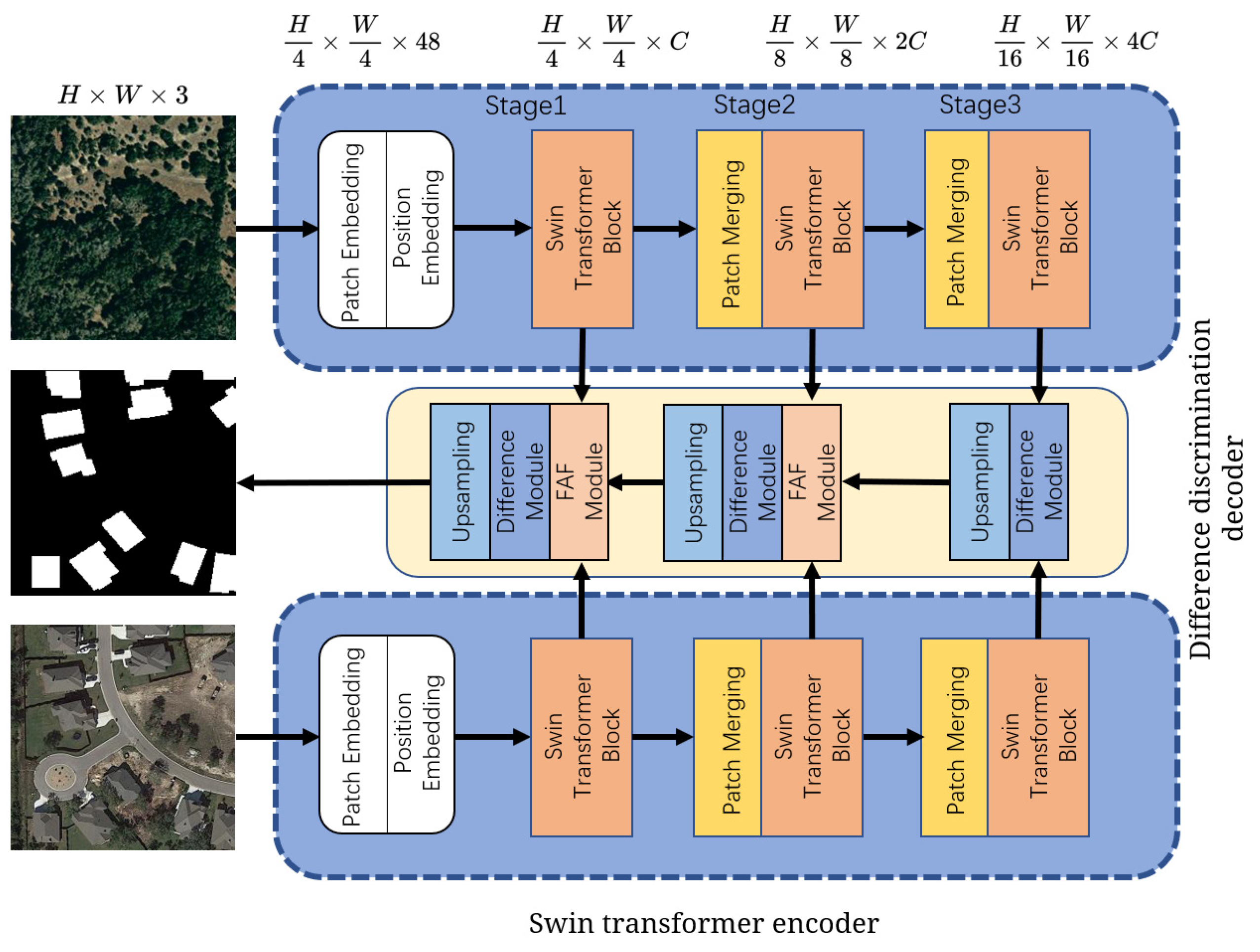
• To increase the detection ability of the model for small target changes without introducing too many parameters and computational overhead, and to balance the local and global sensory fields, we introduce the Swin transformer in the change detection coding path and propose a VHR dual-time remote-sensing image change detection network based on the Swin transformer.
• We designed a FAF module based on a soft attention mechanism, which guides the trimming of low-level feature responses using high-level features to make the model focus more on the change region in the decoding path, reducing the impact of complex backgrounds and irrelevant changes.
• We designed a series of experiments to validate our design and further explore and discuss the model. Based on these experiments, the parameters and structure of the standard model were adjusted to introduce a lightweight version.

The remainder of this paper is organized as follows. Section 2 describes the proposed network design. Section 3 tests the performance of our network. We also compare the performance of SFCD with several SOTA algorithms on two public datasets. Section 4 discusses the role of different components, the effect of parameters in the Swin transformer encoder on accuracy, and the efficiency of the model, proposes a lightweight version of the design, and offers future perspectives. Section 5 summarizes the paper and gives the conclusions.

2. Methodology

In this section, we propose a CD network based on a Swin transformer, the overall architecture of which is shown in Figure 1. It is composed of an encoder consisting of a Swin transformer and a decoder consisting of a difference discrimination network. Specifically, the bi-temporal RS images are first passed through a hierarchical Siamese Swin transformer network for multi-scale feature extraction. Subsequently, in the difference discrimination network, we fuse the obtained multi-scale feature maps through the FAF to obtain the change maps by up-sampling the reduction layer by layer.

Section 2.1 and Section 2.2 provide an introduction to the encoder and decoder, respectively, focusing on the Swin transformer and FAF module. The loss function is introduced in Section 2.3.

2.1. Swin Transformer Encoder

To be able to better apply the pre-trained model of the Swin transformer on ImageNet-1k, we tried to keep the structure of the Swin transformer when designing the encoder. As shown in Figure 1, the Swin transformer mainly consists of patch embedding [48], position embedding, a Swin transformer block, and patch merging. The remotely sensed images are mapped into tokens with location information of dimension C by patch embedding and position embedding, and then semantic information of different levels is obtained by feature extraction in three stages. Except for the first stage, each stage consists of a patch-merging layer and several Swin transformer blocks, where patch merging is usually set before the Swin transformer block to reduce the resolution and adjust the number of channels to form a hierarchical design. In order to better preserve the details and positioning information of the images and to take advantage of its hierarchical design, our encoder retains the output results of each stage to facilitate subsequent interfacing with our FAF module to supplement the high-level semantic information. We will focus on the Swin transformer block and shifted-window design in Section 2.1.1 and Section 2.1.2.

In addition, we discarded the last stage of the original Swin transformer, as compressing the feature map size by pursuing too much global RF could lead to the loss of semantic information of dense small targets in the process of compressing the feature map [53]. Additionally, the number of channels gradually increases as the feature map size is reduced, introducing more trainable parameters and making the model more difficult to train and prone to overfitting. This was validated in this study and is discussed in Section 4.3.

2.1.1. Swin Transformer Block

The structure of the Swin transformer block is shown in Figure 2. It consists of LayerNorm (LN) layers, a multi-head self-attention (MSA) module, a residual connection, and a two-layer MLP with nonlinear GELU in between. The window-based MSA (W-MSA) and the shifted-window-based MSA (SW-MSA) modules alternate in two consecutive blocks. Based on this window division mechanism, the successive rotating transformer blocks can be represented as:

$$\begin{array}{l}{\widehat{\mathit{z}}}^l=W-MSA\left(LN\left({\mathit{z}}^{l-1}\right)\right)+{\mathit{z}}^{l-1}\\ {\mathit{z}}^l=\mathrm{MLP}\left(LN\left({\widehat{\mathit{z}}}^l\right)\right)+{\widehat{\mathit{z}}}^l\\ {\widehat{\mathit{z}}}^{l+1}=SW-MSA\left(LN\left({\mathit{z}}^l\right)\right)+{\mathit{z}}^l\\ {\mathit{z}}^{l+1}=\mathrm{MLP}\left(LN\left({\widehat{\mathit{z}}}^{l+1}\right)\right)+{\widehat{\mathit{z}}}^{l+1}\end{array}$$

(1)

where ${\widehat{\mathit{z}}}^l$ and ${\mathit{z}}^l$ denote the output features of the (S)W-MSA and MLP modules for block $l$, respectively. We will explain the design and principles of W-MSA and SW-MSA further on.

2.1.2. Shifted-Window Design

The core self-attentive mechanism of the transformer [32] can be described as:

$$Attention\left(Q,K,V\right)=softmax\left(\frac{Q{K}^T}{\sqrt{d}}\right)V$$

(2)

where matrixes Q, K, and V denote the query, key, and value, respectively, obtained by subjecting the input to a linear transformation matrix; d is a scaling factor used to avoid the gradient disappearance caused by the softmax function.

This attention mechanism allows for modeling between globally arbitrary features, free from the limitations of local RF on the modeling capability. Consequently, its model computation grows quadratically with the sequence length. Therefore, when introduced into the CV field, simply feeding each pixel directly as a feature into the model, as when using convolution, would lengthen the sequence and introduce a huge computational effort. A Swin transformer uses self-attention within the local window to solve this problem. The windows were arranged such that the images were uniformly segmented in a non-overlapping manner. Assuming that each window contains $M\times M$ patches, the computational complexity of the global self-attention module and the attention module of the window based on $h\times w$ block images are:

$$\Omega \left(MSA\right)=4hw{C}^2+2{(hw)}^{2}C$$

(3)

$$\Omega \left(\mathrm{W}\text{-}MSA\right)=4hw{C}^2+2M^{2}hwC$$

(4)

From the above equation, it can be seen that when $M$ is fixed, using self-attentiveness within a local window reduces the model complexity from quadratic to linear in the patched number $hw$.

However, at the same time, window partitioning cuts off the information interaction between features in different windows. The Swin transformer further introduces the shifted-window partitioning method to compensate for this loss. The details are shown in Figure 3. However, it can also be seen that sliding generates more windows, leading to a rebound in computational complexity, and that the new windows vary in size, which also poses a challenge for self-attention computation at a uniform scale.

Therefore, we used feature shift splicing to make it possible to calculate the attention of adjacent regions while maintaining the size and number of the original windows. As shown in Figure 4a, we moved region A from the top-left corner to the bottom-right corner, region B from left to right, and region C from top to bottom. Figure 4b,c shows the corresponding positions of different regions before and after splicing, and the window is reduced from the original 9 to 4 again after the splicing and re-division. It can also be seen that due to the splicing operation, originally non-adjacent regions compute attention within the same window (e.g., feature maps from four different regions are spliced together in the bottom right window of (c)), which may mislead the direction of model learning. To ensure the semantic relevance of adjacent regions, the Swin transformer introduces a special masking method that ignores the attention between non-adjacent regions. After computation, regions A, B, and C were moved back to their original positions to ensure the integrity of the feature map for subsequent operations.

2.2. Difference Discrimination Decoder

The difference discrimination decoder is also composed of three stages. Except for the bottom connection, it consists of a foreground-aware fusion module, a difference module, and an up-sampling module. Since the bottom connection does not need to fuse deeper information, it consists of only the difference module and the up-sampling module.

Figure 5 illustrates the specific design of the foreground-aware module-based difference discrimination decoder, where shallow features from the skip connection and deep features are simultaneously fed into the FAF module for feature pruning and information fusion, and subsequently, the pruned and fused features are fed into multiple difference modules for further decoding. The up-sampling module consists of a transposed convolution initialized by bilinear interpolation and a ReLU activation function, which will not be expanded upon here. The FAF module and the disparity module are explained in detail below.

2.2.1. FAF Module

Since the shallow-level features of the coding path contain the detailed semantic information required for the decoding path, but at the same time, they also contain a large amount of background information that is useless or even interferes with the detection task, and there are semantic inconsistencies between the features of different levels, the fusion of high-level and low-level features in the coding and decoding paths through simple skip connections and channel splicing alone is likely to lead to the foreground (change region) information at important locations being overwhelmed by the background information of irrelevant regions. The semantic inconsistency between levels and the further interaction between complex background information and irrelevant changes will make this problem more serious and cannot satisfy the enhancement of the segmentation effect on the edges of local areas or changing objects.

After further analysis of the skipping structure, it was found that the fusion processing module is too simple to process the features in the codec paths, and directly fusing the unprocessed differential features of the coding part with the deeper differential features will mix the irrelevant information with each other, which is not conducive to the effective supplementation of the detailed information to the deeper semantics, thus causing the feature acquisition and fusion in the hopping stage of the network to be imperfect. To solve the problem of differential feature transfer and fusion between coding and decoding paths by simple hopping, the generated multi-scale features are better utilized for further performance improvement. Here, we further introduce the idea of spatial attention [21], and by modifying it and combining it with channel attention, we designed a FAF module based on soft spatial attention gating [52] to guide the integration of different semantic features in the context of the fusion phase in the codec path of the change detection network. The structure of the FAF module is schematically shown in Figure 5. It mainly consists of a differential attention-gating (DAG) module and an SE module. By optimizing its internal structure, it enhances the fusion of high-level semantic features with spatially important detail information to achieve a more effective feature utilization effect, reduces the semantic inconsistency between different levels, and further improves the change detection performance for small targets and the segmentation performance for the edges of changing objects.

As shown in Figure 5, the inputs to the module are the shallow and deep features at the corresponding locations in the codec path. During processing, the two branches on the input side first adjust the channels of the input features to the same dimension using a 1 × 1 × 1 convolutional processing unit. Then, the soft attention-gating coefficients representing different degrees of spatial location importance are obtained by an additive attention processing unit consisting of pairwise summation, a ReLU activation function, a convolution module, and a sigmoid normalization function. Then, the shallow features are adjusted and filtered with the obtained attention-gating coefficients to obtain a shallow output representation adjusted to different spatial location importance levels under the supervision of the deep features of the encoding path. The resulting adjusted shallow output representation is then channel stitched with the deep features, and the impact of each channel is adjusted using the SE module [20,21]. The overall processing flow of the FAF module can be represented by Equations (5) to (8):

$$F^l=F_{post}^l-F_{pre}^l$$

(5)

$$z_{att}=Sigmoid\left(W_m\left(ReLU\left(W_h{F}_{diff}^{l-1}+W_l{F}^l\right)\right)\right)$$

(6)

$${\widehat{F}}^l=F^l\times z_{att}$$

(7)

$$F_{in}^l=SE(cat({\widehat{F}}^l{}_l,F_{diff}^{l-1}))$$

(8)

where $F_{pre}^l$ and $F_{post}^l$ denote the intermediate layer feature map of the $l$th stage of the bi-temporal RS image obtained from the encoder; $F_{diff}^{l-1}$ denotes the deep-layer feature map obtained by up-sampling on the $l-1$ stage; $W_h$, $W_l$, and $W_m$ correspond to the parameter matrixes in the three convolution blocks in AG; and $z_{att}$ is the obtained weight matrix. $F_{in}^l$ is the input of the difference module, which is also the output of the FAF module.

2.2.2. Difference Module

The cropped and fused feature maps obtained by the FAF module and further processed in the difference module are shown in Figure 5. The difference module consists of multiple difference blocks, and each difference block consists of convolutional layers, BN layers, ReLU, Dropout, and residual connections. Assuming that each difference module contains N difference blocks, the processing flow of the difference module can be represented by Equations (9) and (10):

$$F_{cov-k}^l=Dropout\left(ReLU(BN(W_{cov-k}{F}_{in-k}^l\right))) 1\le k\le N$$

(9)

$$F_{out-k}^l=F_{cov-k}^l+F_{in-k}^l 1\le k\le N$$

(10)

where $F_{in-k}^l$ is the input of the $k$th difference block in the input of the $l$th difference module, $F_{cov-k}^l$ denotes the output result after convolution, the BN layer, ReLU, and Dropout, $W_{cov-k}$ denotes the parameter matrix of the convolution block in the kth difference block, and $F_{out-k}^l$ is the result sent to the up-sampling module after merging the residual connections. The output $F_{out-N}^l$ of the last difference block in each difference module becomes the deep feature of the next stage after up-sampling and activation, which can be expressed by Equation (11):

$$F_{out-k}^l=F_{cov-k}^l+F_{in-k}^l 1\le k\le N$$

(11)

In the difference discrimination decoder used in this study, the number of difference blocks in the difference module connected at the bottom of the number of difference blocks is 3, and the number of difference blocks in the subsequent two stages of the difference module is 3 and 2, respectively.

2.3. Loss Function

In the training stage, we minimized the cross-entropy loss to optimize the network parameters. Formally, the loss function is expressed as:

$$L={\displaystyle \sum }_{h=1,w=1}^{H,W}l\left(P_{hw},Y_{hw}\right)/\left(H_0\times W_0\right)$$

(12)

where $l\left(P_{hw},Y_{hw}\right)$ = $-log\left(P_{hwy}\right)$ is the cross-entropy loss, and $Y_{hw}$ is the label for the pixel at location (h, w).

3. Experiments and Results

3.1. Datasets

In this section, we present the datasets used in this study. We used the open-source change detection dataset widely used in previous studies to compare our model more intuitively and fairly with other deep-learning methods. In addition, we did not select only the same type of dataset as some other studies. To comprehensively evaluate the change detection effectiveness of our method on different ground feature types, we selected the dataset LEVIR-CD to reflect changes in buildings and the dataset CDD to reflect changes in land cover objects. The examples of the two datasets are shown in Figure 6.

3.1.1. LEVIR-CD

LEVIR-CD [23] is a large-scale remotely sensed building change detection (CD) dataset that provides a new benchmark for evaluating CD algorithms, especially those based on deep learning. The dataset includes 637 VHR (0.5 m/pixel) Google Earth image patch pairs covering various types of buildings, such as villa homes, tall apartments, small garages, and large warehouses. The annotations focus on building-related changes, including building growth and decline. The dataset contains a total of 31,333 individual instances of changing buildings, which we divided into 7120/1024/2048 image pairs of 256 × 256 size for training/validation/testing according to their default dataset partitioning.

3.1.2. CCD

CDD [54] is a change detection dataset focusing on changes in different land cover objects. The dataset comprises 11 pairs of satellite images acquired in different seasons, with resolutions ranging from 0.03 m/pixel to 1 m/pixel. The annotations of changed regions consist of objects varying in size and category, including cars, roads, and construction. Seven images have a size of 4725 × 2200, and four images are 1900 × 1000. After rotation and cropping, the dataset is divided into 10,000/3000/3000 pairs of 256 × 256 size for training/validation/testing purposes.

3.2. Evaluation Metrics

We used the F1 score and Intersection over Union (IoU) [55] associated with the change category as the main evaluation metrics. In addition, we report the accuracy and recall of the change categories and the overall accuracy (OA) performance of the change detection task. The IoU and F1 scores are calculated as follows, where TP denotes true positives, FP denotes false positives, and FN denotes false negatives:

$$IoU=TP/\left(TP+FP+FN\right)$$

(13)

$$F1=2\times (\mathrm{precision} \times \mathrm{recall})/(\mathrm{precision} + \mathrm{recall})$$

(14)

The precision is calculated as follows:

$$precision=TP/\left(TP+FP\right)$$

(15)

The recall is calculated as follows:

$$recall=TP/\left(TP+FN\right)$$

(16)

The OA is calculated as follows:

$$OA=\left(TP+TN\right)/\left(TP+FN+TN+FP\right)$$

(17)

3.3. Implementation Details

Our model was implemented using PyTorch and trained using an NVIDIA Tesla RTX 5000 GPU. We applied conventional data enhancements to the input image blocks, including random rotation, random flip, Gaussian blur, and color dithering, while normalizing both datasets on each of the two respective time phases to speed up the model convergence. We used pre-trained weights from the Swin transformer trained on the ImageNet-1k dataset. We used the AdamW optimizer to optimize the model, with the learning rate initially set to 1 × 10⁻⁴, linearly decaying to 0 over 200 epochs, and the batch set to 16. We performed a validation after each training cycle and evaluated the test set using the best model on the validation set. We minimized the cross-entropy loss to optimize the network parameters.

3.4. Comparison with Other Methods

We compared our model with the best-performing models on two datasets, including four purely convolution-based methods (FC-EF, FC-Siam-diff, FC-Siam-conc [9], UNet++ MSOF [16]), six attention-based methods (DTCDSCN [22], STANet [23], IFNet [8], SNUNet [17], DASNet [24], and RDP-Net [56]), five transformer-based methods (BIT [44], ChangeFormer [46], UVACD [45], SARAS-Net [27], and STCD [29]), and a generating adversarial network (GAN [56])-based method [14]. It is worth stating that since RDP-Net does not publish its specific strategy for classifying datasets, we did not use its proposed efficient training method when reproducing its model on LEVIR-CD. In addition, SARAS-Net is entered as 512 × 512 in its open-source implementation, and we chose its version using resnet18 as the backbone.

3.4.1. Experimental Results Obtained on the LEVIR-CD Dataset

Table 1. Results on the LEVIR-CD dataset (the highest scores are in bold; all values are reported as percentages (%)).

Method	F1	IoU	Precision	Recall	OA
FC-EF	83.40	71.53	86.91	80.17	98.39
FC-Siam-conc	83.69	71.96	91.99	76.77	98.49
FC-Siam-diff	86.31	75.92	89.53	83.31	98.67
DTCDSCN	87.67	78.05	88.53	86.83	98.77
STANet	87.26	77.40	83.81	91.00	98.66
IFNet	88.13	78.77	94.02	82.93	98.87
SNUNet	88.16	78.83	89.18	87.17	98.82
BIT	89.31	80.68	89.24	89.37	98.92
ChangeFormer	90.40	82.48	92.05	88.80	99.04
UVACD	91.30	83.98	91.90	90.70	99.12
RDP-Net	88.77	79.81	88.43	89.11	98.86
SARAS-Net	90.40	82.49	91.48	89.35	98.95
STCD	89.85	81.58	92.91	86.99	—
SFCD (ours)	91.78	84.81	90.79	92.80	99.17

shows the results of SFCD compared with some previous CD algorithms on the LEVIR-CD datasets. It can be seen that on the LEVIR-CD dataset, our method improves the F1 score and IoU by 0.49% and 0.83%, respectively, compared with the previous SOTA method UVACD. Our model also achieves the best performance in all metrics except for precision.

To further visually evaluate our model, we plotted some inferred results of several methods in the test set based on the work of Bandara and Patel [46], including several benchmark methods and the baseline method FC-Siam-diff. Because UVACD and STCD have not currently provided open-source code, they were not compared. The results are shown in Figure 7. For a clearer view, different colors are used to denote TP (white), TN (black), FP (red), and FN (blue). We can observe that the model based on SFCD achieved better results compared to the other models.

Specifically, for the changes in the building, as shown in Figure 7a, our model can avoid the interference caused by the pseudo-change in the local complex scene and better restore the outline of the entire completed area of the building. In addition, as shown by the red box in Figure 7b, although the labels are not successfully shown, we can still see in the original image that at time B, two small houses were added in the red box relative to time A. Compared to other models that could detect at most one of them, our model could capture the change intact. This shows that our model can achieve very good results in detecting changes in both local large-scale and small targets.

3.4.2. Experimental Results Obtained on the CCD Dataset

Table 2. Results on CDD dataset (the highest scores are in bold; all values are reported as percentages (%)).

Method	F1	IoU	Precision	Recall	OA
FC-EF	78.26	64.29	68.56	91.17	95.51
FC-Siam-conc	80.68	67.62	73.70	89.12	95.84
FC-Siam-diff	83.48	71.16	75.54	94.18	96.44
DTCDSCN	93.39	87.60	90.90	96.02	98.48
UNet++ MSOF	88.31	79.06	89.54	87.11	96.73
IFN	90.30	82.32	94.96	86.08	97.71
DASNet	91.94	85.09	91.40	92.50	98.20
SNUNet	96.33	92.89	96.27	96.40	99.14
BIT	95.70	91.75	95.59	95.81	98.99
SDACD	97.34	94.83	97.13	97.56	—
RDP-Net	97.21	94.56	97.19	97.23	99.34
SFCD (ours)	97.87	95.82	98.21	97.53	99.50

shows the results of SFCD compared with some previous CD algorithms on the CDD datasets. As can be seen, SFCD also shows an excellent performance on this dataset. Compared to the previous SOTA method, SDACD, our method improved the F1 score and the IoU by 0.53% and 0.99%. Except for the recall rate, which was 0.03% worse than SDACD in second place, we achieved the best score in all other metrics. Similarly, we visualized the inference results of different models on the CDD dataset, and the results are shown in Figure 8.

As can be seen from Figure 8, although the previous methods can achieve good results, both in the detection effect of the road network in Figure 8a and the detection effect of the cars in Figure 8b,d, our model can detect the changes nearly perfectly, whether these include the shape of the main or branch roads of the road network or the increase or decrease in cars, with almost no misses or misjudgments. In addition, as shown in Figure 8c, our model also maintains the contour shape of the image with less FP compared to other models, which can also avoid the possible pseudo-variation from the shadow area.

4. Discussion

4.1. Ablation Studies

To verify the effectiveness of the different components of our proposed model, we performed ablation experiments on two datasets. The results are shown in

Table 3. Comparison of results of ablation experiments. We used ResNet18 and its pre-trained model on ImageNet-1k as a feature extractor in the model without (w/o) the Swin transformer.

Method	LEVIR-CD			CDD
	F1 (%)	IoU (%)	OA (%)	F1 (%)	IoU (%)	OA (%)
w/o Swin, FAF	90.13	82.04	99.02	95.61	91.59	98.97
w/o Swin	90.56	82.76	99.05	95.94	92.20	99.04
w/o FAF	91.37	84.09	99.13	97.48	95.08	99.40
SFCD	91.78	84.81	99.17	97.87	95.82	99.50

. The data show that using both the Swin transformer and the FAF module can improve F1 scores by 1.65% and 2.26% and the IoU by 2.77% and 4.23% for LEVIR-CD and CCD, respectively. Using a Swin transformer alone can improve the F1 scores by 1.24% and 1.87%, respectively, and using the FAF module in addition to the Swin transformer further improves F1 scores by 0.41% and 0.39%.

In addition, to further analyze whether our module achieves the expected results, we plotted the inference of the standard model and the model with the Swin transformer removed on the two test sets separately in Figure 9. As shown in Figure 9, the standard SFCD has better results in small target and edge change detection and segmentation compared to the model without the Swin transformer. It is worth noting that using the Swin transformer in the feature extraction stage can better avoid the omission of small target changes at the image edges, as shown in Figure 9a. This is because the pixels near the target are crucial for target identification, and the missing information around the target at the image edges makes discrimination more difficult. The Swin transformer, based on the self-attentive mechanism, can avoid such problems to the maximum extent by making fuller use of the available information within the image and its larger RF. This is very important for the change detection task of remote sensing, as remote-sensing images are usually huge, and the current graphics cards do not support operations on such large images. Therefore, the images are usually cropped for practical use, so the situation in Figure 9a often occurs in the change detection of remote-sensing images.

Figure 10 shows the difference in the feature activation maps of the skip connection before and after using the FAF module. In the figure, we can see that the feature activation of the change class in the skip connection is very weak before using the FAF module, indicating that the skip connection is less helpful for the final correct classification at this time. In contrast, after using the FAF module, the feature activation in the change region is significantly enhanced, and there is almost no change in the no-change (background) region, thus enhancing the foreground filtering of the background. The experimental results show that our design is effective, and both strategies can optimize the model independently.

4.2. Parameter Analysis of Swin Transformer Encoder

Unlike ordinary images, a large number of dense small targets often appear in RS images; therefore, we revisited the impact of global attention. We hypothesized that compressing the feature map size by pursuing the global RF too much may result in the semantic information of dense small targets being lost in the process of compressing the feature map. The feature map will gradually become deeper as the feature map size is reduced, thus introducing more trainable parameters and making the model more difficult to train and prone to overfitting. We conducted experiments using the LEVIR-CD and CDD datasets by adjusting the number of blocks and stages of the Swin transformer with the same total architecture, and the results are shown in

Table 4. Performance of SFCD for different block/stage numbers on LEVIR-CD and CDD test sets.

Block/Stage	LEVIR-CD			CDD
	F1 (%)	IoU (%)	OA (%)	F1 (%)	IoU (%)	OA (%)
(2,2)	90.85	83.23	99.08	97.44	95.01	99.39
(2,2,2)	91.39	84.41	99.13	97.71	95.52	99.46
(2,2,6)	91.78	84.81	99.17	97.87	95.82	99.50
(2,2,6,2)	91.63	84.55	99.16	97.91	95.90	99.51

. We can observe that the model gains more improvement when the model is changed from two stages to three stages, which might be because increasing the stages when the model is shallow can fully increase the complexity and RF of the model, thus gaining better modeling capability. However, as the number of model layers continues to increase, it can be seen that when the number of stages is changed from three to four, there is almost no improvement in F1 scores and IoU on both datasets, and the model degrades to some extent on LEVIR-CD. This degradation might be because the size of the dataset is not sufficient for the increased training difficulty caused by the increase in the number of parameters or the overfitting of the model due to the excessive parameter size. Meanwhile, since the six-layer Swin transformer block is used in the third stage, given its sliding-window mechanism, it already has an RF close to the global scale. Therefore, adding a stage did not improve this aspect of the model.

However, this decline will improve as the size of the dataset increases and because of the presence of residual connections. Nevertheless, a deeper Swin transformer still has more potential when the data size is sufficient, and the model is well-trained.

4.3. Model Efficiency and Lightweight Version

The current goals of deep learning are higher accuracy, smaller models, and faster running speeds. Therefore, in addition to accuracy, being lightweight is an important goal, especially for change detection. Since some practical applications require change detection on edge devices, such as drones and satellite image processing, lightweight models can be more easily deployed to edge devices. We tested the parametric size and the inference time required for a single image on LEVIR-CD for a better evaluation of our model against some models with better performance.

As can be seen from

Table 5. Comparison of the number of parameters and test time (the best scores are in bold).

Methods	Params (M)	LEVIR-CD		CCD		Test Time (ms)
		F1 (%)	IoU (%)	F1 (%)	IoU (%)
DTCDSCN	41.07	87.67	78.05	93.39	87.60	24.31
UNet++ MSOF	11.00	—	—	88.31	79.06	—
STANet	16.93	87.26	77.40	—	—	25.33
IFNet	50.17	88.13	78.77	90.30	82.32	30.75
DASNet	16.25	88.16	78.83	91.94	85.09	29.27
SNUNet	13.21	89.31	80.68	96.33	92.89	46.45
BIT	3.55	90.40	82.48	95.70	91.75	16.54
ChangeFormer	41.29	90.40	82.48	—	—	40.89
SDACD	50.40	—	—	97.34	94.83	—
UVACD	>25.63	91.30	83.98	—	—	—
RDP-Net	1.70	88.77	79.81	97.21	94.56	15.66
SARAS-Net	—	90.40	82.49	—	—	92.68
STCD	9.26	89.85	81.58	—	—	—
SFCD (ours)	17.84	91.78	84.81	97.84	95.78	18.25
SFCD-mi(ours)	1.55	90.46	82.58	97.30	94.79	15.54

, our model is moderately sized and achieves a 2.33% improvement in the F1 score approximately 60% fewer parameters compared to previous transformer-based approaches, such as ChangeFormer, that achieved excellent results. For UVACD, although it is not open-source, we can infer that its number of parameters may be much larger than 25.63 M, because it uses the full resnet50 as well as the transformer and ASPP. Therefore, our model showed a huge improvement in all metrics. Our standard model’s performance in inference speed is also noteworthy. It was almost greater than some lightweight methods such as BIT and RDP-Net, for which the number of parameters and inference time of our model seem to be disadvantages. In order to broaden the usage of our model and make it more flexible and applicable under various scenarios, it is necessary to introduce a lightweight version of SFCD. From the discussion of the parameters in Section 4.2, we can see that even with a two-stage Swin transformer, we can still achieve very good results while maintaining the overall architecture of our model. Based on this, we took a two-stage Swin transformer to extract features and replaced the convolution blocks in the decoder with deeply separable convolutions [57] to obtain a lighter version of SFCD.

We evaluated the obtained lighter version of SFCD-mini and have placed the results in the last row of Table 5. As can be seen, SFCD-mini can reduce the number of parameters of the model to 1/12 of the original one at the expense of 1.32% of the F1 score. Compared to the other two lightweight models, BIT and RDP-Net, SFCD-mini has fewer parameters and a lower inference time but performs better in all metrics. Even when comparing all the methods, SFCD-mini can stay within the top three in F1 score and IoU, with the smallest number of parameters and lowest inference time. It further proves the flexibility of our proposed method as well as its application scope and the effectiveness of our design.

4.4. Future Work Outlook

At present, most CD models are based on supervised learning, which involves training with paired input and output data (i.e., samples and their corresponding labels). The use of labels has a dual impact: supervised learning can leverage label information to learn more accurate predictions, resulting in higher accuracy when the training and testing data distributions are similar. However, label information also makes the model more directional, limiting its generalization ability to some extent. Consequently, when facing data with a significantly different distribution from the training set, the performance of supervised learning models may decline substantially. As a dense prediction task, CD requires relatively expensive annotation efforts. Therefore, enhancing the transferability of deep-learning-based CD methods is also a highly significant research direction. In the remote sensing domain, some researchers have successfully implemented cross-sensor remote-sensing image semantic segmentation using Unsupervised Domain Adaptation (UDA) [58,59], yielding satisfactory results and verifying the feasibility of improving the cross-sensor transferability of different deep-learning models by incorporating UDA.

Furthermore, our study on lightweight CD remains in its early stages. Although the introduction of structured pruning and depth-wise separable convolution to reduce model size is simple and effective, it is rather crude. In future work, we could consider adopting more fine-grained pruning methods [60] to remove less important layers from the model. Similarly, knowledge distillation [61] and model quantization [62] are becoming increasingly mature with ongoing research and could be incorporated into CD tasks to further advance lightweight research.

In conclusion, as deep-learning technology continues to evolve, its integration with remote-sensing technology becomes increasingly close-knit. Exploring how to better utilize deep learning as a tool to address remote-sensing-related tasks will be a meaningful research direction in this field.

5. Conclusions

In this study, a Swin transformer-based dual-stream CD network called SFCD is proposed. It relies on a pair of Swin transformer networks with shared parameters to perform multi-scale feature extraction on bi-temporal RS images. Owing to the excellent performance of self-attention and the hierarchical design of Swin transformers, our model not only has a strong global modeling capability but also significantly improves the CD capability for small targets. In addition, to ensure better utilization of the location and detailed information of the encoding path, we also introduced our designed attention gate-based FAF module in the decoding path, using the result of fusing high-level features with shallow features to guide the adjustment of shallow features, prune low-level feature responses, and further enhance semantic discriminability. However, our approach does not adequately address the cross-sensor transferability issue, which is also prevalent in current change detection methods. Additionally, our research on lightweight models remains relatively superficial, with room for improvement. In our future work, we will further explore appropriate methods to tackle these challenges.

References

1. Kim, Y.; Lee, M.-J. Rapid Change Detection of Flood Affected Area after Collapse of the Laos Xe-Pian Xe-Namnoy Dam using Sentinel-1 GRD Data. Remote Sens. 2020, 12, 1978. [Google Scholar] [CrossRef]
2. Gärtner, P.; Förster, M.; Kurban, A.; Kleinschmit, B. Object based change detection of Central Asian Tugai vegetation with very high spatial resolution satellite imagery. Int. J. Appl. Earth Obs. Geoinf. 2014, 31, 110–121. [Google Scholar] [CrossRef]
3. Hulley, G.; Veraverbeke, S.; Hook, S. Thermal-based techniques for land cover change detection using a new dynamic MODIS multispectral emissivity product (MOD21). Remote Sens. Environ. 2014, 140, 755–765. [Google Scholar] [CrossRef]
4. Khan, S.; He, X.; Porikli, F.; Bennamoun, M. Forest Change Detection in Incomplete Satellite Images with Deep Neural Networks. IEEE Trans. Geosci. Remote Sens. 2017, 55, 5407–5423. [Google Scholar] [CrossRef]
5. Jaturapitpornchai, R.; Matsuoka, M.; Kanemoto, N.; Kuzuoka, S.; Ito, R.; Nakamura, R. Newly Built Construction Detection in SAR Images Using Deep Learning. Remote Sens. 2019, 11, 1444. [Google Scholar] [CrossRef]
6. Wu, C.; Zhang, L.; Du, B. Kernel Slow Feature Analysis for Scene Change Detection. IEEE Trans. Geosci. Remote Sens. 2017, 55, 2367–2384. [Google Scholar] [CrossRef]
7. Al rawashdeh, S. Evaluation of the differencing pixel-by-pixel change detection method in mapping irrigated areas in dry zones. Int. J. Remote Sens. 2011, 32, 2173–2184. [Google Scholar] [CrossRef]
8. Zhang, C.; Yue, P.; Tapete, D.; Jiang, L.; Shangguan, B.; Huang, L.; Liu, G. A deeply supervised image fusion network for change detection in high resolution bi-temporal remote sensing images. ISPRS J. Photogramm. Remote Sens. 2020, 166, 183–200. [Google Scholar] [CrossRef]
9. Daudt, R.C.; Saux, B.L.; Boulch, A. Fully Convolutional Siamese Networks for Change Detection. In Proceedings of the 2018 25th IEEE International Conference on Image Processing (ICIP), Athens, Greece, 7–10 October 2018; pp. 4063–4067. [Google Scholar] [CrossRef]
10. Dong, R.; Pan, X.; Li, F. DenseU-Net-Based Semantic Segmentation of Small Objects in Urban Remote Sensing Images. IEEE Access 2019, 7, 65347–65356. [Google Scholar] [CrossRef]
11. Li, X.; He, H.; Li, X.; Li, D.; Cheng, G.; Shi, J.; Weng, L.; Tong, Y.; Lin, Z. PointFlow: Flowing Semantics Through Points for Aerial Image Segmentation. In Proceedings of the 2021 IEEE/CVF Conference on Computer Vision and Pattern Recognition (CVPR), Nashville, TN, USA, 20–25 June 2021; pp. 4215–4224. [Google Scholar]
12. Deng, Z.; Sun, H.; Zhou, S.; Zhao, J. Learning Deep Ship Detector in SAR Images from Scratch. IEEE Trans. Geosci. Remote Sens. 2019, 57, 4021–4039. [Google Scholar] [CrossRef]
13. Pang, J.; Li, C.; Shi, J.; Xu, Z.; Feng, H. Fast Tiny Object Detection in Large-Scale Remote Sensing Images. IEEE Trans. Geosci. Remote Sens. 2019, 57, 5512–5524. [Google Scholar] [CrossRef]
14. Liu, J.; Xuan, W.; Gan, Y.; Zhan, Y.; Liu, J.; Du, B. An End-to-end Supervised Domain Adaptation Framework for Cross-Domain Change Detection. Pattern Recognit. 2022, 132, 108960. [Google Scholar] [CrossRef]
15. Lin, M.; Yang, G.; Zhang, H. Transition Is a Process: Pair-to-Video Change Detection Networks for Very High Resolution Remote Sensing Images. IEEE Trans. Image Process. 2022, 32, 57–71. [Google Scholar] [CrossRef] [PubMed]
16. Peng, D.; Zhang, Y.; Guan, H. End-to-End Change Detection for High Resolution Satellite Images Using Improved UNet++. Remote Sens. 2019, 11, 1382. [Google Scholar] [CrossRef]
17. Fang, S.; Li, K.; Shao, J.; Li, Z. SNUNet-CD: A Densely Connected Siamese Network for Change Detection of VHR Images. IEEE Geosci. Remote Sens. Lett. 2021, 19, 8007805. [Google Scholar] [CrossRef]
18. Wang, H.; Cao, P.; Wang, J.; Zaïane, O. UCTransNet: Rethinking the Skip Connections in U-Net from a Channel-Wise Perspective with Transformer. Proc. AAAI Conf. Artif. Intell. 2022, 36, 2441–2449. [Google Scholar] [CrossRef]
19. Blaschke, T. Object based image analysis for remote sensing. ISPRS J. Photogramm. Remote Sens. 2010, 65, 2–16. [Google Scholar] [CrossRef]
20. Hu, J.; Shen, L.; Sun, G. Squeeze-and-Excitation Networks. In Proceedings of the 2018 IEEE/CVF Conference on Computer Vision and Pattern Recognition, Salt Lake City, UT, USA, 18–23 June 2018; pp. 7132–7141. [Google Scholar]
21. Woo, S.; Park, J.; Lee, J.-Y.; Kweon, I. CBAM: Convolutional Block Attention Module. In Proceedings of the European Conference on Computer Vision (ECCV), Munich, Germany, 8–14 September 2018; pp. 3–19. [Google Scholar]
22. Liu, Y.; Pang, C.; Zhan, Z.; Zhang, X.; Yang, X. Building Change Detection for Remote Sensing Images Using a Dual-Task Constrained Deep Siamese Convolutional Network Model. IEEE Geosci. Remote Sens. Lett. 2020, 18, 811–815. [Google Scholar] [CrossRef]
23. Chen, H.; Shi, Z. A Spatial-Temporal Attention-Based Method and a New Dataset for Remote Sensing Image Change Detection. Remote Sens. 2020, 12, 1662. [Google Scholar] [CrossRef]
24. Chen, J.; Yuan, Z.; Peng, J.; Chen, L.; Huang, H.; Zhu, J.; Liu, Y.; Li, H. DASNet: Dual Attentive Fully Convolutional Siamese Networks for Change Detection in High-Resolution Satellite Images. IEEE J. Sel. Top. Appl. Earth Obs. Remote Sens. 2021, 14, 1194–1206. [Google Scholar] [CrossRef]
25. Peng, X.; Zhong, R.; Li, Z.; Li, Q. Optical Remote Sensing Image Change Detection Based on Attention Mechanism and Image Difference. IEEE Trans. Geosci. Remote Sens. 2020, 59, 7296–7307. [Google Scholar] [CrossRef]
26. Chen, L.; Zhang, D.; Li, P.; Lv, P. Change Detection of Remote Sensing Images Based on Attention Mechanism. Comput. Intell. Neurosci. 2020, 2020, 6430627. [Google Scholar] [CrossRef] [PubMed]
27. Chen, C.-P.; Hsieh, J.-W.; Chen, P.-Y.; Hsieh, Y.-K.; Wang, B.-S. SARAS-Net: Scale and Relation Aware Siamese Network for Change Detection. arXiv 2022, arXiv:2212.01287. [Google Scholar] [CrossRef]
28. Chen, P.; Hong, D.; Chen, Z.; Yang, X.; Li, B. FCCDN: Feature constraint network for VHR image change detection. ISPRS J. Photogramm. Remote Sens. 2022, 187, 101–119. [Google Scholar] [CrossRef]
29. Wang, D.; Chen, X.; Guo, N.; Yi, H.; Li, Y. STCD: Efficient Siamese transformers-based change detection method for remote sensing images. Geo-Spat. Inf. Sci. 2023, 1–20. [Google Scholar] [CrossRef]
30. He, K.; Zhang, X.; Ren, S.; Sun, J. Deep Residual Learning for Image Recognition. In Proceedings of the IEEE Conference on Computer Vision and Pattern Recognition (CVPR), Las Vegas, NV, USA, 27–30 June 2016; pp. 770–778. [Google Scholar]
31. Simonyan, K.; Zisserman, A. Very Deep Convolutional Networks for Large-Scale Image Recognition. arXiv 2014, arXiv:1409.1556. [Google Scholar]
32. Vaswani, A.; Shazeer, N.; Parmar, N.; Uszkoreit, J.; Jones, L.; Gomez, A.; Kaiser, L.; Polosukhin, I. Attention Is All You Need. arXiv 2017, arXiv:1706.03762. [Google Scholar]
33. Dosovitskiy, A.; Beyer, L.; Kolesnikov, A.; Weissenborn, D.; Zhai, X.; Unterthiner, T.; Dehghani, M.; Minderer, M.; Heigold, G.; Gelly, S.; et al. An Image is Worth 16x16 Words: Transformers for Image Recognition at Scale. arXiv 2020, arXiv:2010.11929. [Google Scholar]
34. Wu, B.; Wang, S.; Yuan, X.; Wang, C.; Rudolph, C.; Yang, X. Defeating Misclassification Attacks Against Transfer Learning. IEEE Trans. Dependable Secur. Comput. 2023, 20, 886–901. [Google Scholar] [CrossRef]
35. Playout, C.; Duval, R.; Boucher, M.C.; Cheriet, F. Focused Attention in Transformers for interpretable classification of retinal images. Med. Image Anal. 2022, 82, 102608. [Google Scholar] [CrossRef]
36. Chen, J.; Lu, Y.; Yu, Q.; Luo, X.; Adeli, E.; Wang, Y.; Lu, L.; Yuille, A.; Zhou, Y. TransUNet: Transformers Make Strong Encoders for Medical Image Segmentation. arXiv 2021, arXiv:2102.04306. [Google Scholar]
37. Chen, W.; Du, X.; Yang, F.; Beyer, L.; Zhai, X.; Lin, T.-Y.; Chen, H.; Li, J.; Song, X.; Wang, Z.; et al. A Simple Single-Scale Vision Transformer for Object Detection and Instance Segmentation. In Computer Vision–ECCV 2022; Springer: Cham, Switzerland, 2022; pp. 711–727. [Google Scholar]
38. Esser, P.; Rombach, R.; Ommer, B. Taming Transformers for High-Resolution Image Synthesis. In Proceedings of the 2021 IEEE/CVF Conference on Computer Vision and Pattern Recognition (CVPR), Nashville, TN, USA, 20–25 June 2021; pp. 12868–12878. [Google Scholar]
39. Lee, K.; Chang, H.; Jiang, L.; Zhang, H.; Tu, Z.; Liu, C. ViTGAN: Training GANs with Vision Transformers. arXiv 2021, arXiv:2107.04589. [Google Scholar]
40. Gao, M.; Yang, Q.F.; Ji, Q.X.; Wu, L.; Liu, J.; Huang, G.; Chang, L.; Xie, W.; Shen, B.; Wang, H.; et al. Probing the Material Loss and Optical Nonlinearity of Integrated Photonic Materials. In Proceedings of the 2021 Conference on Lasers and Electro-Optics (CLEO), San Jose, CA, USA, 9–14 May 2021; pp. 1–2. [Google Scholar]
41. Liang, T.; Chu, X.; Liu, Y.; Wang, Y.; Tang, Z.; Chu, W.; Chen, J.; Ling, H. CBNetV2: A Composite Backbone Network Architecture for Object Detection. arXiv 2021, arXiv:2107.00420. [Google Scholar]
42. Fang, Y.; Yang, S.; Wang, S.; Ge, Y.; Shan, Y.; Wang, X. Unleashing Vanilla Vision Transformer with Masked Image Modeling for Object Detection. arXiv 2022, arXiv:2204.02964. [Google Scholar]
43. Sun, M.; Huang, X.; Sun, Z.; Wang, Q.; Yao, Y. Unsupervised Pre-training for 3D Object Detection with Transformer. In Proceedings of the Pattern Recognition and Computer Vision, Shenzhen, China, 4–7 November 2022; pp. 82–95. [Google Scholar]
44. Chen, H.; Shi, Z.; Qi, Z. Remote Sensing Image Change Detection with Transformers. IEEE Trans. Geosci. Remote Sens. 2021, 60, 5607514. [Google Scholar] [CrossRef]
45. Wang, G.; Li, B.; Zhang, T.; Zhang, S. A Network Combining a Transformer and a Convolutional Neural Network for Remote Sensing Image Change Detection. Remote Sens. 2022, 14, 2228. [Google Scholar] [CrossRef]
46. Bandara, W.G.C.; Patel, V.M. A Transformer-Based Siamese Network for Change Detection. In Proceedings of the IGARSS 2022–2022 IEEE International Geoscience and Remote Sensing Symposium, Kuala Lumpur, Malaysia, 17–22 July 2022; pp. 207–210. [Google Scholar]
47. Mohammadian, A.; Ghaderi, F. SiamixFormer: A Siamese Transformer Network for Building Detection And Change Detection From Bi-Temporal Remote Sensing Images. arXiv 2022, arXiv:2208.00657. [Google Scholar] [CrossRef]
48. Liu, Z.; Lin, Y.; Cao, Y.; Hu, H.; Wei, Y.; Zhang, Z.; Lin, S.; Guo, B. Swin Transformer: Hierarchical Vision Transformer using Shifted Windows. In Proceedings of the 2021 IEEE/CVF International Conference on Computer Vision (ICCV), Montreal, QC, Canada, 11–17 October 2021; pp. 9992–10002. [Google Scholar]
49. Cao, H.; Wang, Y.; Chen, J.; Jiang, D.; Zhang, X.; Tian, Q.; Wang, M. Swin-Unet: Unet-like Pure Transformer for Medical Image Segmentation. arXiv 2021, arXiv:2105.05537. [Google Scholar]
50. Hatamizadeh, A.; Nath, V.; Tang, Y.; Yang, D.; Roth, H.; Xu, D. Swin UNETR: Swin Transformers for Semantic Segmentation of Brain Tumors in MRI Images. arXiv 2022, arXiv:2201.01266. [Google Scholar]
51. Xiao, X.; Guo, W.; Chen, R.; Hui, Y.; Wang, J.; Zhao, H. A Swin Transformer-Based Encoding Booster Integrated in U-Shaped Network for Building Extraction. Remote Sens. 2022, 14, 2611. [Google Scholar] [CrossRef]
52. Oktay, O.; Schlemper, J.; Folgoc, L.; Lee, M.; Heinrich, M.; Misawa, K.; Mori, K.; McDonagh, S.; Hammerla, N.; Kainz, B.; et al. Attention U-Net: Learning Where to Look for the Pancreas. arXiv 2018, arXiv:1804.03999. [Google Scholar]
53. Chen, L.-C.; Papandreou, G.; Schroff, F.; Adam, H. Rethinking Atrous Convolution for Semantic Image Segmentation. arXiv 2017, arXiv:1706.05587. [Google Scholar]
54. Lebedev, M.; Vizilter, Y.; Vygolov, O.; Knyaz, V.; Rubis, A. Change detection in remote sensing images using conditional adversarial networks. ISPRS Int. Arch. Photogramm. Remote Sens. Spat. Inf. Sci. 2018, XLII-2, 565–571. [Google Scholar] [CrossRef]
55. Everingham, M.; Van Gool, L.; Williams, C.K.I.; Winn, J.; Zisserman, A. The Pascal Visual Object Classes (VOC) Challenge. Int. J. Comput. Vis. 2010, 88, 303–338. [Google Scholar] [CrossRef]
56. Chen, H.; Pu, F.; Yang, R.; Rui, T.; Xu, X. RDP-Net: Region Detail Preserving Network for Change Detection. arXiv 2022, arXiv:2202.09745. [Google Scholar] [CrossRef]
57. Chollet, F. Xception: Deep Learning with Depthwise Separable Convolutions. In Proceedings of the 2017 IEEE Conference on Computer Vision and Pattern Recognition (CVPR), Honolulu, HI, USA, 21–26 July 2017; pp. 1800–1807. [Google Scholar]
58. Wang, J.; Ma, A.; Zhong, Y.; Zheng, Z.; Zhang, L. Cross-sensor domain adaptation for high spatial resolution urban land-cover mapping: From airborne to spaceborne imagery. Remote Sens. Environ. 2022, 277, 113058. [Google Scholar] [CrossRef]
59. Li, Y.; Shi, T.; Zhang, Y.; Chen, W.; Wang, Z.; Li, H. Learning deep semantic segmentation network under multiple weakly-supervised constraints for cross-domain remote sensing image semantic segmentation. ISPRS J. Photogramm. Remote Sens. 2021, 175, 20–33. [Google Scholar] [CrossRef]
60. Liu, Z.; Li, J.; Shen, Z.; Huang, G.; Yan, S.; Zhang, C. Learning Efficient Convolutional Networks through Network Slimming. In Proceedings of the 2017 IEEE International Conference on Computer Vision (ICCV), Venice, Italy, 22–29 October 2017; pp. 2755–2763. [Google Scholar]
61. Hinton, G.; Vinyals, O.; Dean, J.J.C.S. Distilling the Knowledge in a Neural Network. arXiv 2015, arXiv:1503.02531. [Google Scholar]
62. Jacob, B.; Kligys, S.; Chen, B.; Zhu, M.; Tang, M.; Howard, A.; Adam, H.; Kalenichenko, D. Quantization and Training of Neural Networks for Efficient Integer-Arithmetic-Only Inference. In Proceedings of the 2018 IEEE/CVF Conference on Computer Vision and Pattern Recognition, Salt Lake City, UT, USA, 18–23 June 2018; pp. 2704–2713. [Google Scholar]
Figure 1. The overall architecture of the proposed SFCD.
Remotesensing 15 02645 g001
Figure 2. Two successive Swin transformer blocks, W-MSA and SW-MSA, are multi-head self-attention modules with regular and shifted windowing configurations, respectively.
Remotesensing 15 02645 g002
Figure 3. Two different window-partitioning strategies used. In layer l (a), a regular window-partitioning scheme is adopted, and self-attention is computed within each window. In the next layer l + 1 (b), the window partitioning is shifted, resulting in new windows. The self-attention computation in the new windows crosses the boundaries of the previous windows in layer l , providing connections among them.
Remotesensing 15 02645 g003
Figure 4. Illustration of an efficient batch computation approach of the feature map: (a) cyclic shift, (b) window partition, (c) feature shift splicing. Same color indicates corresponding areas.
Remotesensing 15 02645 g004
Figure 5. The structure of one stage of the difference discrimination network.
Remotesensing 15 02645 g005
Figure 6. Examples of cropped LEVIR-CD and CDD datasets (a) from LEVIR-CD and (b) from CDD. Time A and time B are bi-temporal images, respectively, Ground Truth is the manually marked area of change, white shows a changed region, and black shows an unchanged region.
Remotesensing 15 02645 g006
Figure 7. Comparison of visualization results of different methods on the LEVIR-CD test set. (a,b) show different image pairs that were analyzed. The images are color-coded as follows: white shows true positive, black shows true negative, red shows false positive, and blue shows false negative.
Remotesensing 15 02645 g007
Figure 8. Comparison of visualization results of different methods on the CDD test sets. (ad) show different image pairs that were analyzed. The images are color-coded as white for true positive, black for true negative, red for false positive, and blue for false negative.
Remotesensing 15 02645 g008
Figure 9. Inference comparison with/without Swin transformer. From left to right (ae): time A images, time B images, Ground Truth maps, inference of SFCD, inference of the model without Swin transformer.
Remotesensing 15 02645 g009
Figure 10. Feature activation before and after using the FAF module for skip connection. From left to right (ae): time A images, time B images, Ground Truth maps, feature activation before using FAF module, feature activation after using FAF module.
Remotesensing 15 02645 g010