


An Efficient Cloud Classification Method Based on a Densely Connected Hybrid Convolutional Network for FY-4A


Abstract
1. Introduction
2. Data
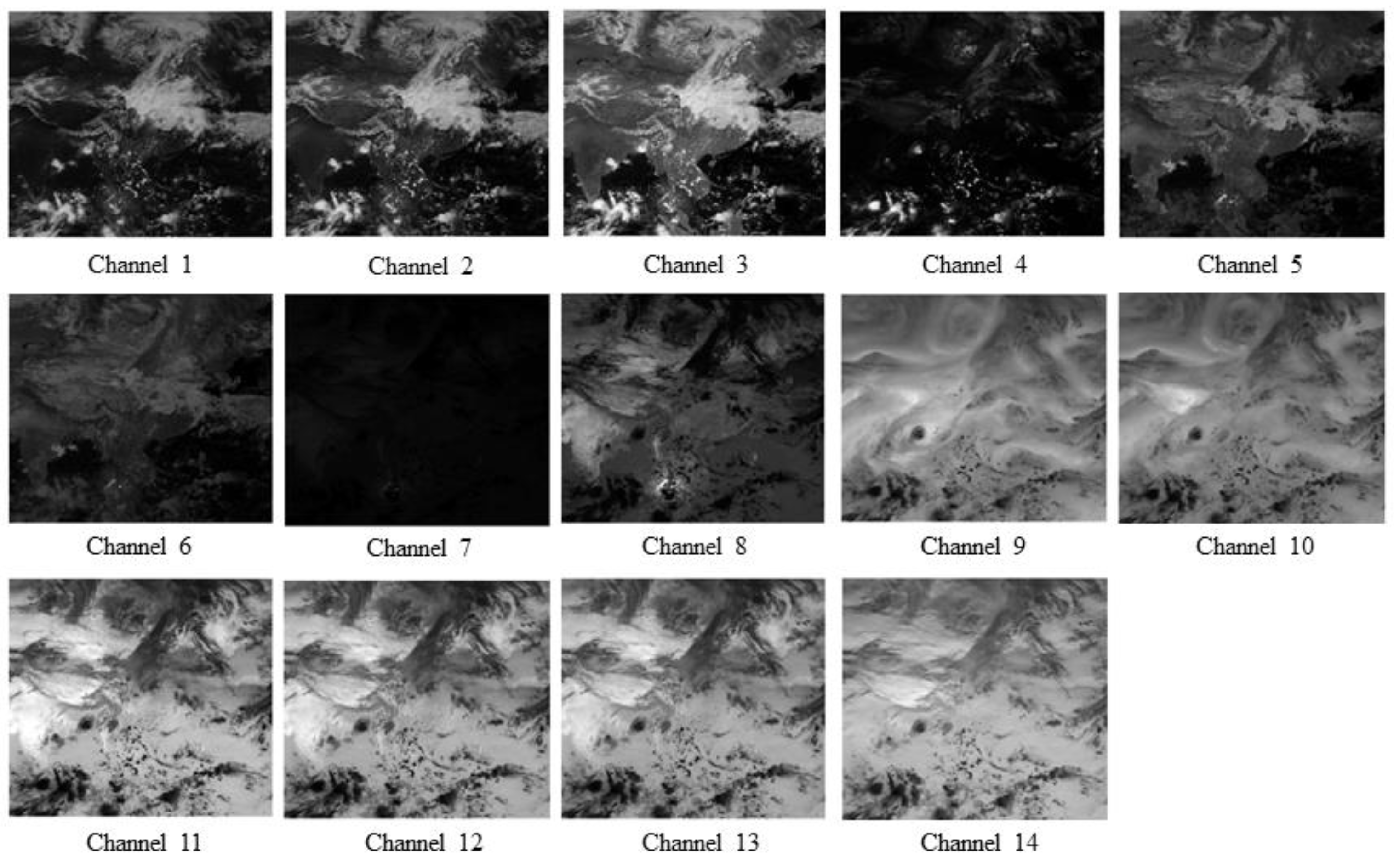
2.1. FY-4A Data
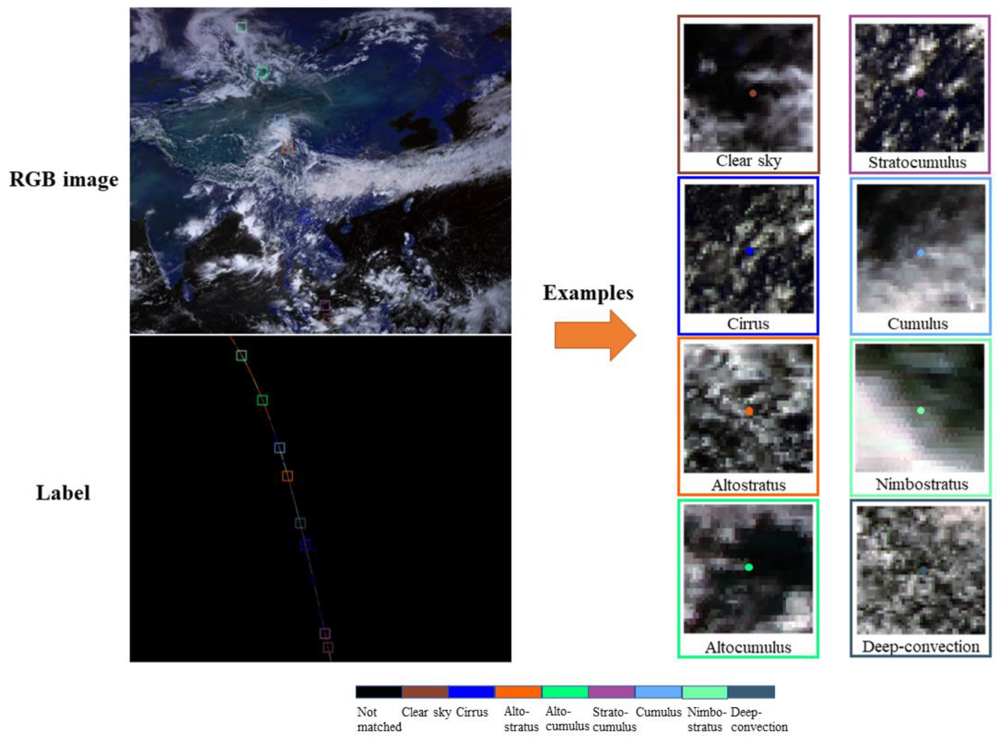
2.2. Cloudsat Data for Inspection
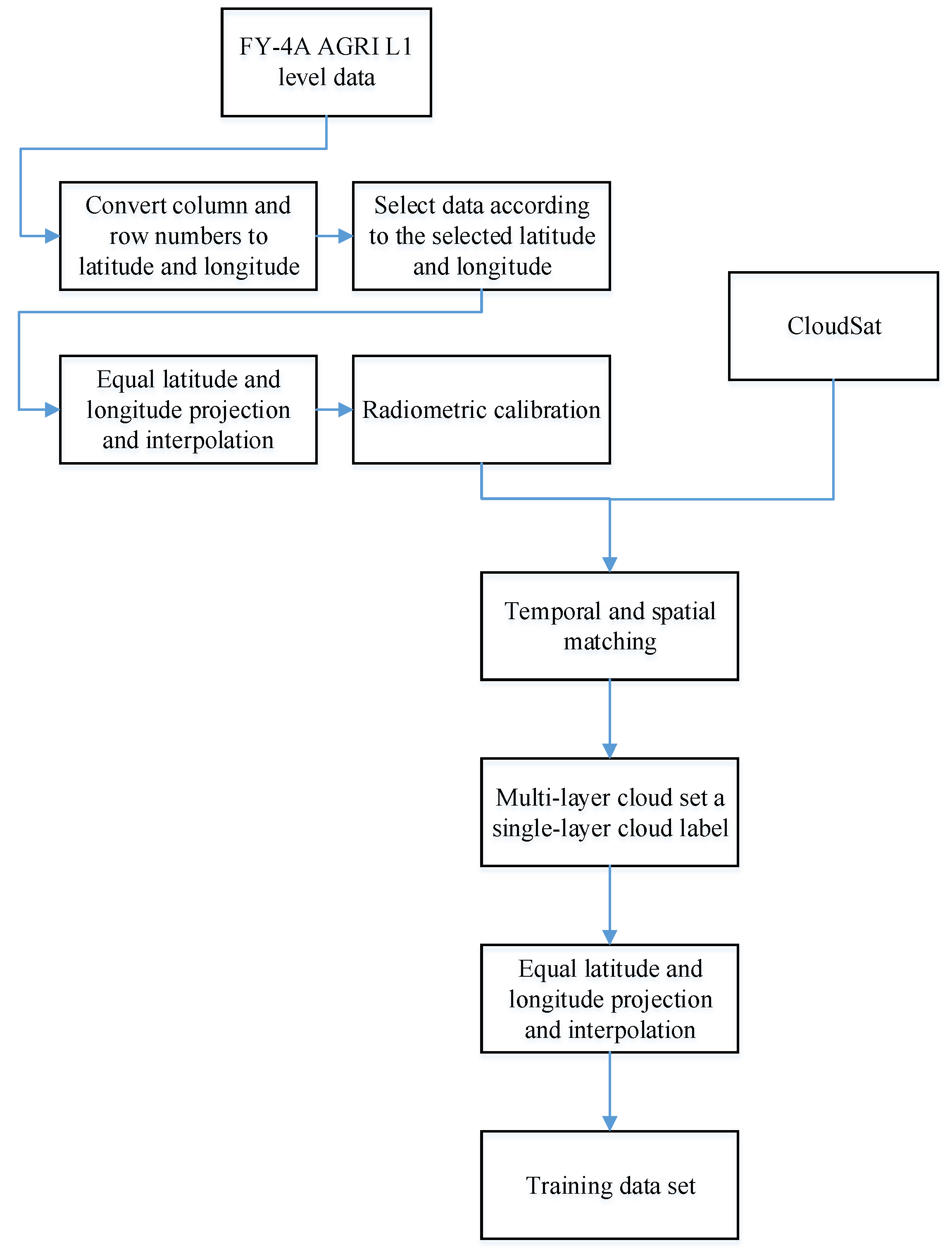
2.3. Data Preprocessing
3. Methods
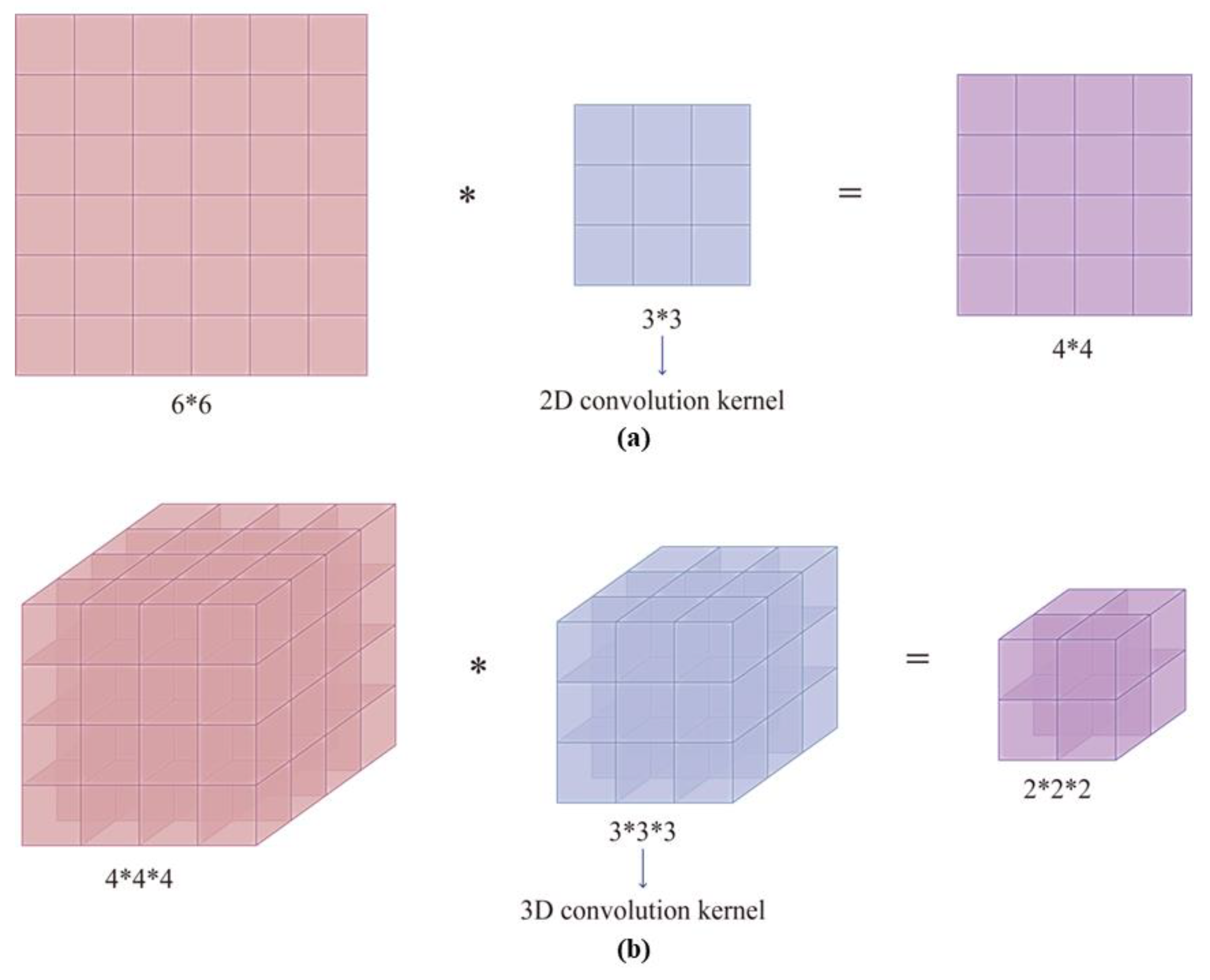
3.1. Superiority of Proposed Module
3.2. Proposed DCHCN Method
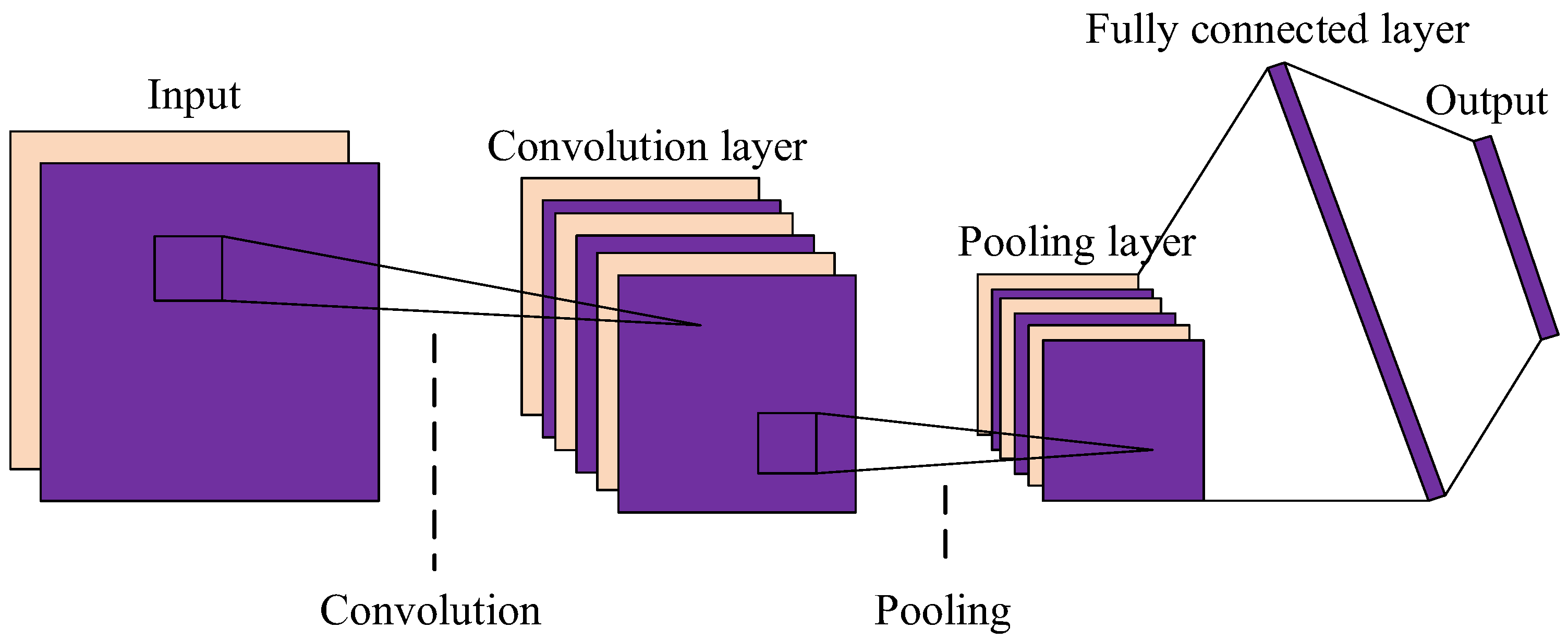
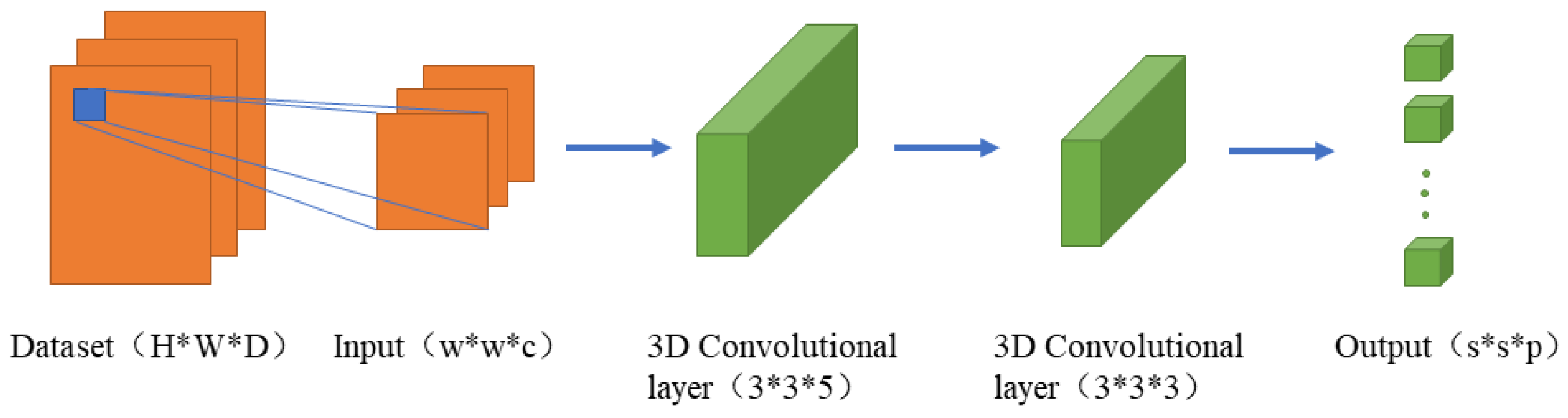
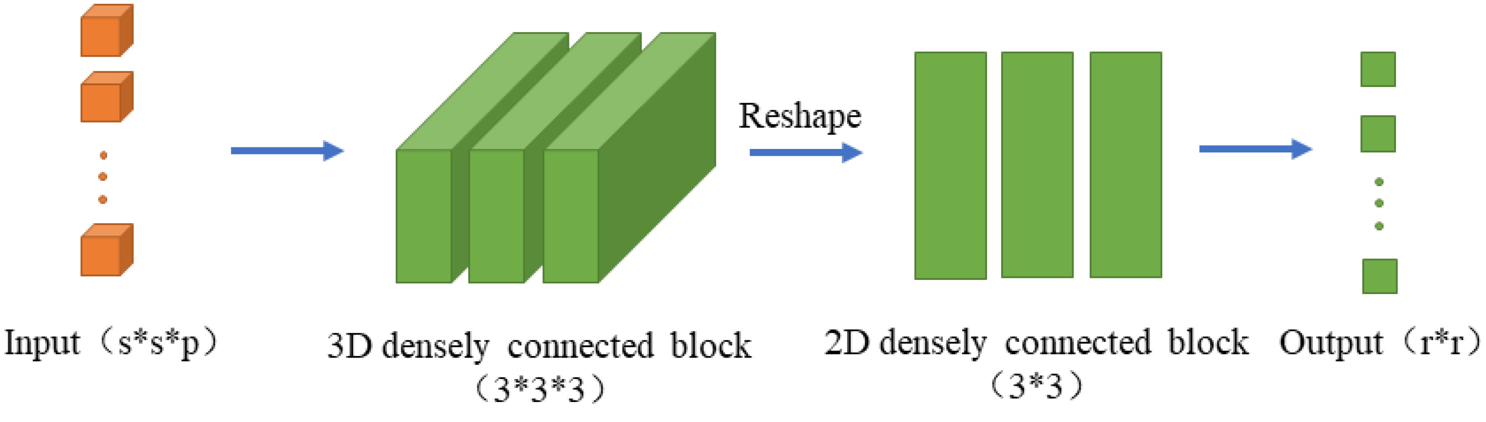
3.2.1. Using the 3D-CNN for Extracting Spatial–Spectral Features
- (1)
- To satisfy the 3D-CNN input data format, the original dataset needs to be chunked. Each pixel in the original dataset is traversed, and each pixel is centered to obtain an image block with a size of , where is the width of the image block, i.e., the window size, and is the number of channels. The label of the input block is equivalent to the label of the center pixel, and the resulting input block is represented by ;
- (2)
- For an input block with a size of {}, the output with a size of {} is obtained by processing the data using eight 3D convolution kernels with a size of {}. The first layer of 3D convolution is used to filter the joint spatial spectral features and remove the channels that may contain noise. The second 3D convolution layer consists of 16 convolution kernels with a size of {}, extracts the features further, and has an output with a size of {}. After two 3D convolutions, the extraction process of 3D features is initially completed. The step size of the above-mentioned convolution layers is one;
- (3)
- To prevent the network from overfitting and to improve the convergence speed, a batch normalization (BN) layer and a ReLU function are added after each convolution to enhance model robustness.
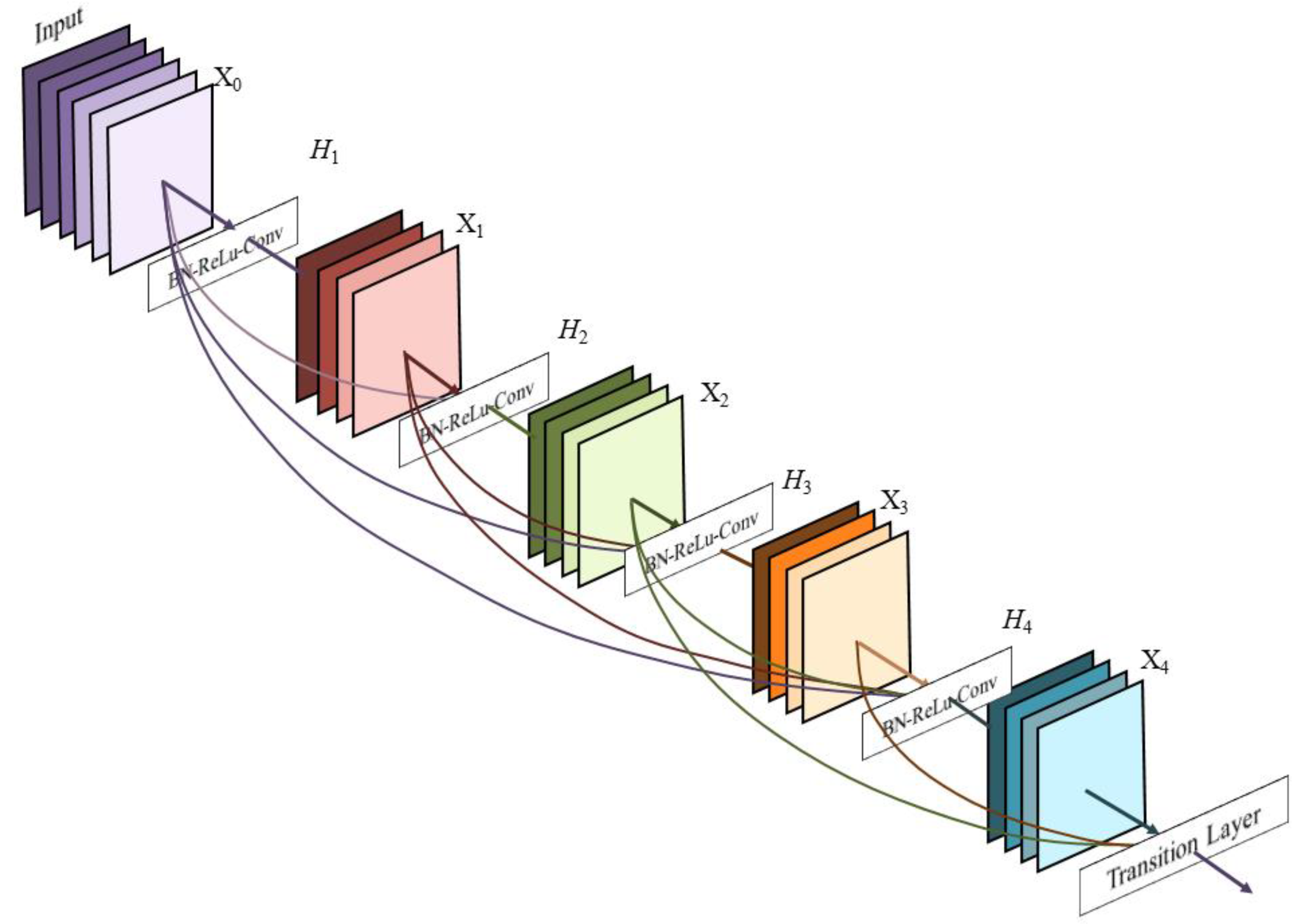
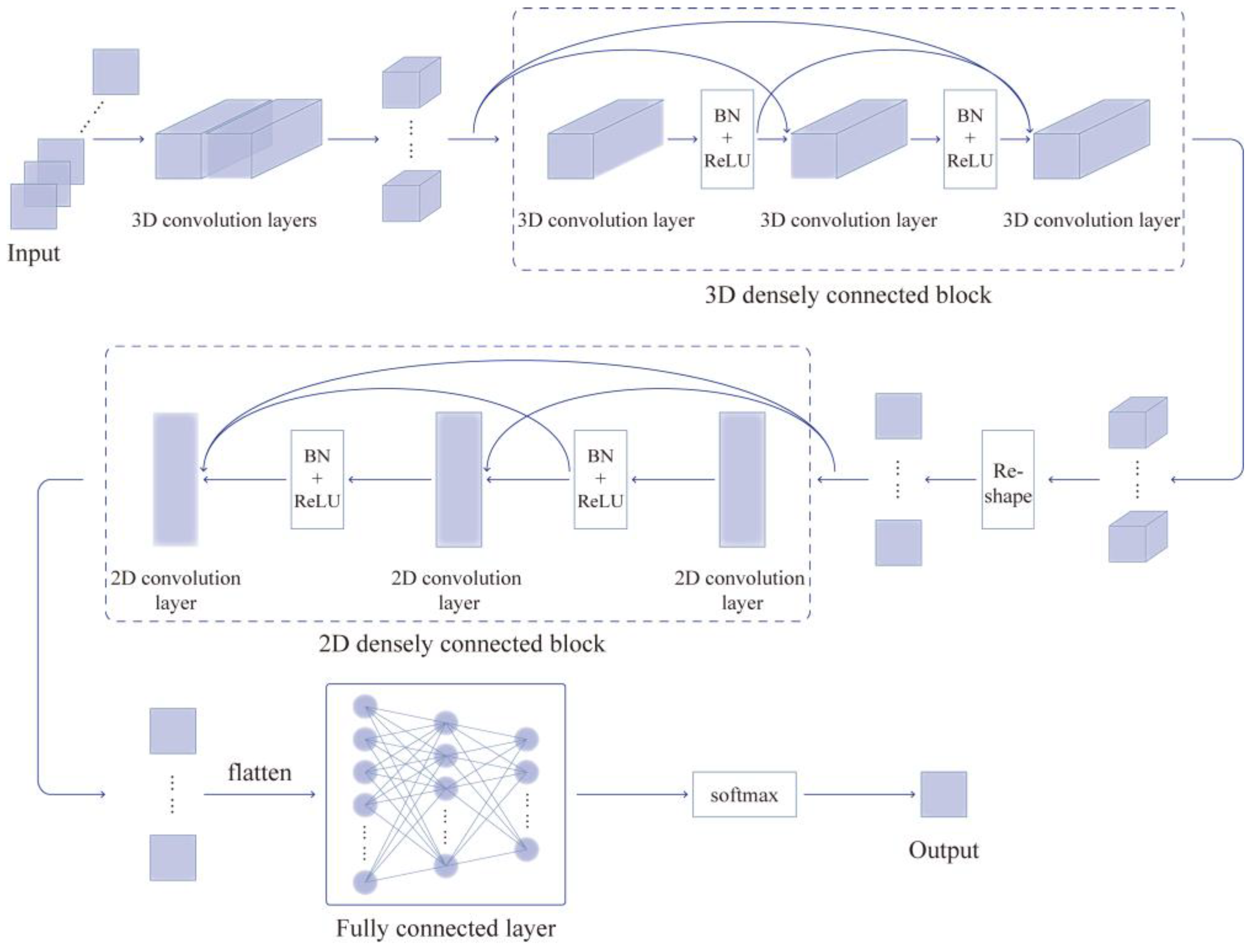
3.2.2. Hybrid Convolutional Layers with Dense Connections
- (1)
- The 3D densely connected block includes three convolutional layers, each of which is convolved in 3D. Each layer has a convolutional kernel with a size of {} and uses a BN layer and a ReLU function for non-linear transformation between layers to avoid overfitting problems. For the {} input, the size of the convolutional layers’ output is guaranteed to be the same by setting the padding to 1 to ensure that the output of each layer can be passed to all subsequent layers. The input is first processed by 16 convolutional kernels with a size of {}, and the output is fed to the next layer by splicing it with the input using the concatenate operation (the channel splicing method). To reduce the number of parameters of the 3D densely connected block, the number of output channels is set to 16 for each layer;
- (2)
- The output obtained using the 3D densely connected block is obtained by screening and capturing the spectral feature information, and the spatial feature map is obtained using 2D convolution. The dimensionality is reduced using the reshape operation to facilitate 2D convolution. The input of size {} is passed through 32 convolution kernels with a size of {} to extract the spatial features, and the output with a size of {} is obtained to construct the input size that can be fed to the 2D densely connected block;
- (3)
- The 2D densely connected block has three 2D convolutional layers, each of which has a convolutional kernel with a size of {}, using the BN layer and ReLU function for non-linear transformation between layers to avoid the overfitting problem. For the {} input, the output size of the convolutional layers is guaranteed to be the same by setting the padding to one and thus ensuring that the output of each layer can be passed to all subsequent layers. First, the input is passed through 32 convolutional kernels with a size of {}, and the obtained output is input to the next layer by splicing it with the input performing the concatenation operation (the channel splicing method). For a better exploration of spatial features, the number of output channels is set to 32 for each layer.
3.2.3. Fully Connected Layers for Classification
3.3. Model Training
4. Result and Analysis
4.1. Experimental Configuration
4.2. Analysis of Parameter Effects on Model Performance
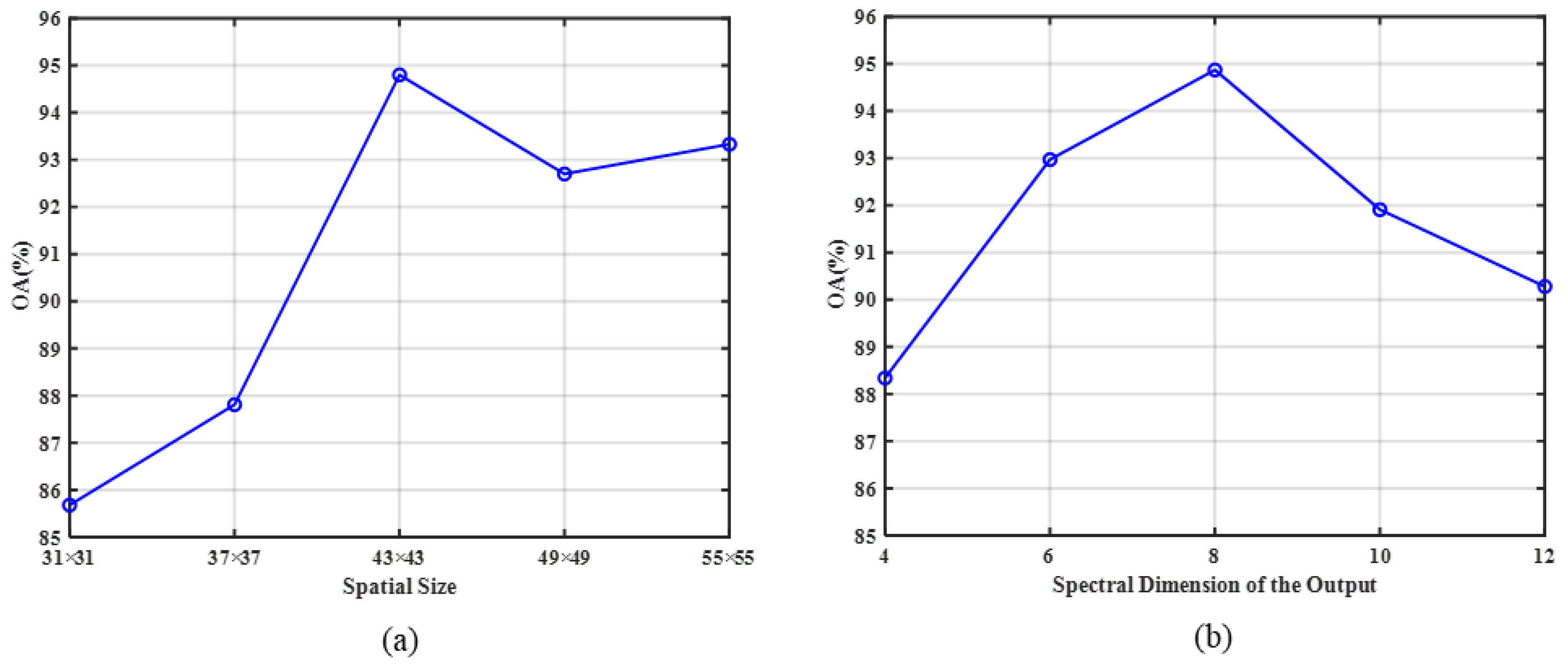
4.2.1. Spatial Size Effect
4.2.2. Spectral Dimension of the 3D-CNN Output Feature Map
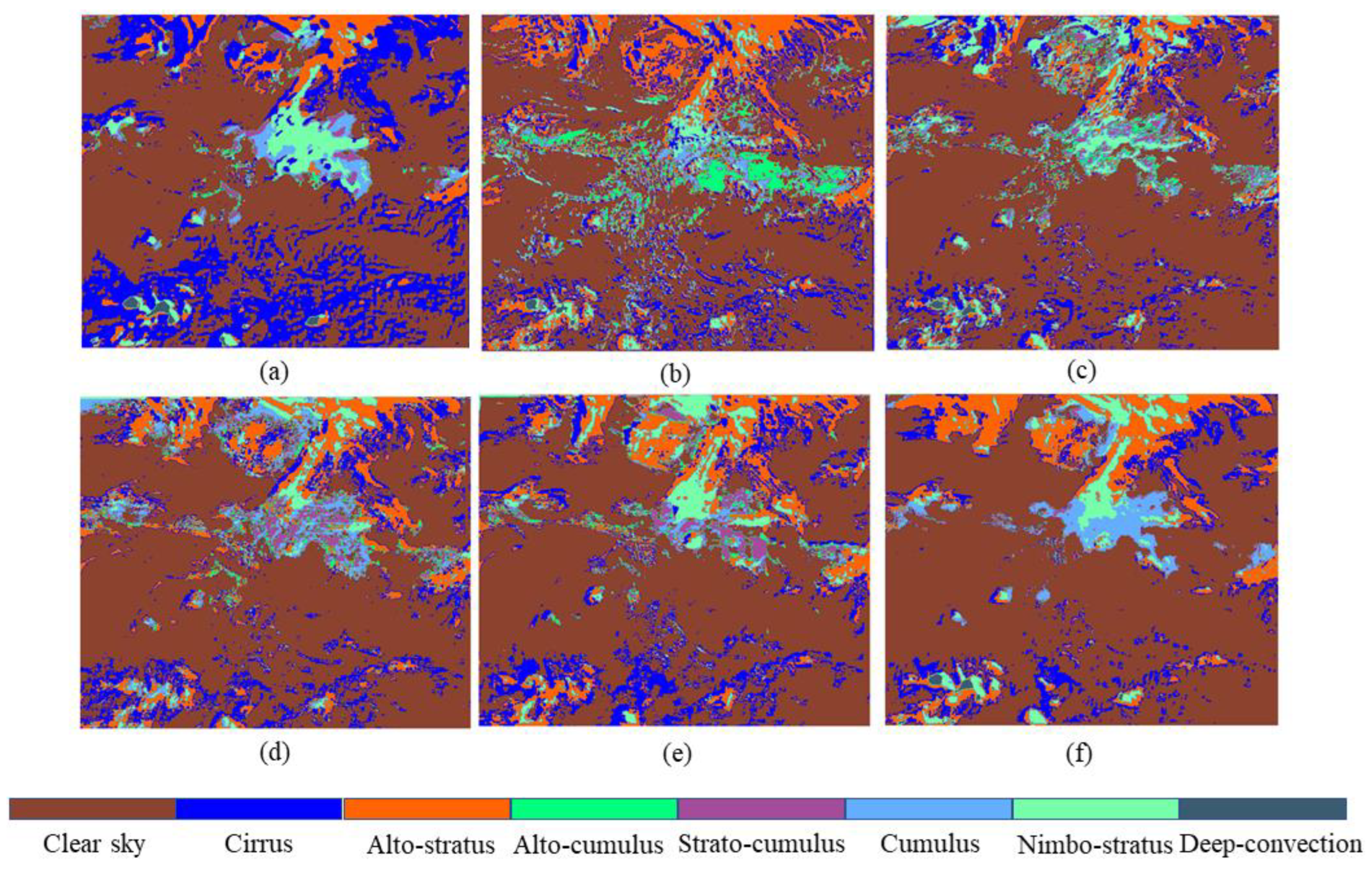
4.3. Results, Analysis, and Comparison of Different Cloud Classification Models
5. Conclusions
Author Contributions
Funding
Data Availability Statement
Acknowledgments
Conflicts of Interest
References
- Hunt, G.E. On the sensitivity of a general circulation model climatology to changes in cloud structure and radiative properties. Tellus A Dyn. Meteorol. Oceanogr. 1982, 34, 29. [Google Scholar] [CrossRef]
- Baker, M. Cloud microphysics and climate. Science 1997, 276, 1072–1078. [Google Scholar] [CrossRef]
- Liu, Y.; Xia, J.; Shi, C.X.; Hong, Y. An Improved Cloud Classification Algorithm for China’s FY-2C Multi-Channel Images Using Artificial Neural Network. Sensors 2009, 9, 5558–5579. [Google Scholar] [CrossRef]
- Gan, J.; Lu, W.; Li, Q.; Zhang, Z.; Yang, J.; Ma, Y.; Yao, W. Cloud Type Classification of Total-Sky Images Using Duplex Norm-Bounded Sparse Coding. IEEE J. Sel. Top. Appl. Earth Obs. Remote Sens. 2017, 10, 3360–3372. [Google Scholar] [CrossRef]
- Stubenrauch, C.J.; Rossow, W.B.; Kinne, S.; Ackerman, S.; Cesana, G.; Chepfer, H.; Di Girolamo, L.; Getzewich, B.; Guignard, A.; Heidinger, A.; et al. Assessment of Global Cloud Datasets from Satellites: Project and Database Initiated by the GEWEX Radiation Panel. Bull. Am. Meteorol. Soc. 2013, 94, 1031–1049. [Google Scholar] [CrossRef]
- Reichstein, M.; Camps-Valls, G.; Stevens, B.; Jung, M.; Denzler, J.; Carvalhais, N.; Prabhat. Deep learning and process understanding for data-driven Earth system science. Nature 2019, 566, 195–204. [Google Scholar] [CrossRef] [PubMed]
- Huertas-Tato, J.; Rodríguez-Benítez, F.J.; Arbizu-Barrena, C.; Aler-Mur, R.; Galvan-Leon, I.; Pozo-Vázquez, D. Automatic Cloud-Type Classification Based On the Combined Use of a Sky Camera and a Ceilometer. J. Geophys. Res. Atmos. 2017, 122, 11045–11061. [Google Scholar] [CrossRef]
- Li, J.; Menzel, W.P.; Yang, Z.; Frey, R.A.; Ackerman, S.A. High-spatial-resolution surface and cloud-type classification from MODIS multispectral band measurements. J. Appl. Meteorol. Climatol. 2003, 42, 204–226. [Google Scholar] [CrossRef]
- Wang, J.; Liu, C.; Yao, B.; Min, M.; Letu, H.; Yin, Y.; Yung, Y.L. A multilayer cloud detection algorithm for the Suomi-NPP Visible Infrared Imager Radiometer Suite (VIIRS). Remote Sens. Environ. 2019, 227, 1–11. [Google Scholar] [CrossRef]
- Rossow, W.B.; Schiffer, R.A. ISCCP cloud data products. Bull. Am. Meteorol. Soc. 1991, 72, 2–20. [Google Scholar] [CrossRef]
- Hahn, C.J.; Rossow, W.B.; Warren, S.G. ISCCP cloud properties associated with standard cloud types identified in individual surface observations. J. Clim. 2001, 14, 11–28. [Google Scholar] [CrossRef]
- Austin, R.T.; Heymsfield, A.J.; Stephens, G.L. Retrieval of ice cloud microphysical parameters using the CloudSat millimeter-wave radar and temperature. J. Geophys. Res. 2009, 114. [Google Scholar] [CrossRef]
- Powell, K.A.; Hu, Y.; Omar, A.; Vaughan, M.A.; Winker, D.M.; Liu, Z.; Hunt, W.H.; Young, S.A. Overview of the CALIPSO Mission and CALIOP Data Processing Algorithms. J. Atmos. Ocean. Technol. 2009, 26, 2310–2323. [Google Scholar] [CrossRef]
- Kahn, B.; Chahine, M.; Stephens, G.; Mace, G.; Marchand, R.; Wang, Z.; Barnet, C.; Eldering, A.; Holz, R.; Kuehn, R. Cloud type comparisons of AIRS, CloudSat, and CALIPSO cloud height and amount. Atmos. Chem. Phys. 2008, 8, 1231–1248. [Google Scholar] [CrossRef]
- Yan, W.; Han, D.; Zhou, X.K.; Liu, H.F.; Tang, C. Analysing the structure characteristics of tropical cyclones based on CloudSat satellite data. Chin. J. Geophys. 2013, 56, 1809–1824. [Google Scholar] [CrossRef]
- Subrahmanyam, K.V.; Kumar, K.K.; Tourville, N.D. CloudSat Observations of Three-Dimensional Distribution of Cloud Types in Tropical Cyclones. IEEE J. Sel. Top. Appl. Earth Obs. Remote Sens. 2018, 11, 339–344. [Google Scholar] [CrossRef]
- Li, G.L.; Yan, W.; Han, D.; Wang, R.; Ye, J. Applications of the CloudSat Tropical Cyclone Product in Analyzing the Vertical Structure of Tropical Cyclones over the Western Pacific. J. Trop. Meteorol. 2017, 23, 473–484. [Google Scholar] [CrossRef]
- Bankert, R.L.; Mitrescu, C.; Miller, S.D.; Wade, R.H. Comparison of GOES cloud classification algorithms employing explicit and implicit physics. J. Appl. Meteorol. Climatol. 2009, 48, 1411–1421. [Google Scholar] [CrossRef]
- Mouri, K.; Izumi, T.; Suzue, H.; Yoshida, R. Algorithm Theoretical Basis Document of cloud type/phase product. Meteorol. Satell. Cent. Tech. Note 2016, 61, 19–31. [Google Scholar]
- Suzue, H.; Imai, T.; Mouri, K. High-resolution cloud analysis information derived from Himawari-8 data. Meteorol. Satell. Cent. Tech. Note 2016, 61, 43–51. [Google Scholar]
- Ackerman, S.A.; Strabala, K.I.; Menzel, W.P.; Frey, R.A.; Moeller, C.C.; Gumley, L.E. Discriminating clear sky from clouds with MODIS. J. Geophys. Res. Atmos. 1998, 103, 32141–32157. [Google Scholar] [CrossRef]
- Purbantoro, B.; Aminuddin, J.; Manago, N.; Toyoshima, K.; Lagrosas, N.; Sumantyo, J.T.S.; Kuze, H. Comparison of Cloud Type Classification with Split Window Algorithm Based on Different Infrared Band Combinations of Himawari-8 Satellite. Adv. Remote Sens. 2018, 7, 218–234. [Google Scholar] [CrossRef]
- Poulsen, C.; Egede, U.; Robbins, D.; Sandeford, B.; Tazi, K.; Zhu, T. Evaluation and comparison of a machine learning cloud identification algorithm for the SLSTR in polar regions. Remote Sens. Environ. 2020, 248, 111999. [Google Scholar] [CrossRef]
- Ebert, E.E. Analysis of polar clouds from satellite imagery using pattern recognition and a statistical cloud analysis scheme. J. Appl. Meteorol. Climatol. 1989, 28, 382–399. [Google Scholar] [CrossRef]
- Berendes, T.A.; Mecikalski, J.R.; MacKenzie, W.M.; Bedka, K.M.; Nair, U.S. Convective cloud identification and classification in daytime satellite imagery using standard deviation limited adaptive clustering. J. Geophys. Res. 2008, 113. [Google Scholar] [CrossRef]
- Zhang, C.; Yu, F.; Wang, C.; Yang, J. Three-dimensional extension of the unit-feature spatial classification method for cloud type. Adv. Atmos. Sci. 2011, 28, 601–611. [Google Scholar] [CrossRef]
- Gao, T.; Zhao, S.; Chen, F.; Sun, X.; Liu, L. Cloud Classification Based on Structure Features of Infrared Images. J. Atmos. Ocean. Technol. 2011, 28, 410–417. [Google Scholar] [CrossRef]
- Gomez-Chova, L.; Camps-Valls, G.; Bruzzone, L.; Calpe-Maravilla, J. Mean Map Kernel Methods for Semisupervised Cloud Classification. IEEE Trans. Geosci. Remote Sens. 2010, 48, 207–220. [Google Scholar] [CrossRef]
- Heinle, A.; Macke, A.; Srivastav, A. Automatic cloud classification of whole sky images. Atmos. Meas. Tech. 2010, 3, 557–567. [Google Scholar] [CrossRef]
- Taravat, A.; Del Frate, F.; Cornaro, C.; Vergari, S. Neural Networks and Support Vector Machine Algorithms for Automatic Cloud Classification of Whole-Sky Ground-Based Images. IEEE Geosci. Remote Sens. Lett. 2015, 12, 666–670. [Google Scholar] [CrossRef]
- Zhang, J.; Liu, P.; Zhang, F.; Song, Q. CloudNet: Ground-Based Cloud Classification With Deep Convolutional Neural Network. Geophys. Res. Lett. 2018, 45, 8665–8672. [Google Scholar] [CrossRef]
- Jiang, Y.; Cheng, W.; Gao, F.; Zhang, S.; Wang, S.; Liu, C.; Liu, J. A Cloud Classification Method Based on a Convolutional Neural Network for FY-4A Satellites. Remote Sens. 2022, 14, 2314. [Google Scholar] [CrossRef]
- Guo, Q.; Lu, F.; Wei, C.; Zhang, Z.; Yang, J. Introducing the New Generation of Chinese Geostationary Weather Satellites, Fengyun-4. Bull. Am. Meteorol. Soc. 2017, 98, 1637–1658. [Google Scholar] [CrossRef]
- Hawkins, J.; Miller, S.; Mitrescu, C.; L’Ecuyer, T.; Turk, J.; Partain, P.; Stephens, G. Near-Real-Time Applications of CloudSat Data. J. Appl. Meteorol. Climatol. 2008, 47, 1982–1994. [Google Scholar] [CrossRef]
- Sassen, K.; Wang, Z.; Liu, D. Global distribution of cirrus clouds from CloudSat/Cloud-Aerosol Lidar and Infrared Pathfinder Satellite Observations (CALIPSO) measurements. J. Geophys. Res. 2008, 113(D8). [Google Scholar] [CrossRef]
- Stephens, G.L.; Vane, D.G.; Tanelli, S.; Im, E.; Durden, S.; Rokey, M.; Reinke, D.; Partain, P.; Mace, G.G.; Austin, R.; et al. CloudSat mission: Performance and early science after the first year of operation. J. Geophys. Res. 2008, 113. [Google Scholar] [CrossRef]
- Vane, D.; Stephens, G.L. The CloudSat Mission and the A-Train: A Revolutionary Approach to Observing Earth’s Atmosphere. In Proceedings of the 2008 IEEE Aerospace Conference, Big Sky, MT, USA, 1–8 March 2008; pp. 1–5. [Google Scholar]
- Gu, J.; Wang, Z.; Kuen, J.; Ma, L.; Shahroudy, A.; Shuai, B.; Liu, T.; Wang, X.; Wang, G.; Cai, J.; et al. Recent advances in convolutional neural networks. Pattern Recognit. 2018, 77, 354–377. [Google Scholar] [CrossRef]
- Huang, G.; Liu, Z.; Van Der Maaten, L.; Weinberger, K.Q. Densely connected convolutional networks. In Proceedings of the IEEE Conference on Computer Vision and Pattern Recognition, Honolulu, HI, USA, 21–26 July 2017; pp. 4700–4708. [Google Scholar]


| Channel Number | Channel Type | Central Wavelength | Spectral Bandwidth |
|---|---|---|---|
| 1 | VIS/NIR | 0.47 µm | 0.45–0.49 µm |
| 2 | 0.65 µm | 0.55–0.75 µm | |
| 3 | 0.825 µm | 0.75–0.90 µm | |
| 4 | Shortwave IR | 1.375 µm | 1.36–1.39 µm |
| 5 | 1.61 µm | 1.58–1.64 µm | |
| 6 | 2.25 µm | 2.1–2.35 µm | |
| 7 | Midwave IR | 3.75 µm | 3.5–4.0 µm (high) |
| 8 | 3.75 µm | 3.5–4.0 µm (low) | |
| 9 | Water vapor | 6.25 µm | 5.8–6.7 µm |
| 10 | 7.1 µm | 6.9–7.3 µm | |
| 11 | Longwave IR | 8.5 µm | 8.0–9.0 µm |
| 12 | 10.7 µm | 10.3–11.3 µm | |
| 13 | 12.0 µm | 11.5–12.5 µm | |
| 14 | 13.5 µm | 13.2–13.8 µm |
| Category | Name | Number of Samples |
|---|---|---|
| 1 | Clear sky | 6447 |
| 2 | Cirrus | 2553 |
| 3 | Altostratus | 3260 |
| 4 | Altocumulus | 723 |
| 5 | Stratocumulus | 530 |
| 6 | Cumulus | 540 |
| 7 | Nimbostratus | 1550 |
| 8 | Deep-convection | 177 |
| 2D-CNN | 3D-CNN | The Hybrid Convolutional Model | |
|---|---|---|---|
| OA | 87.35 | 90.85 | 92.01 |
| Runtime (s) | 192.6 | 338.7 | 252.8 |
| Layer | Type | Output Shape | Parameter |
|---|---|---|---|
| Input_1 | / | (43, 43, 14, 1) | 0 |
| Conv3d_1 | 3 × 3 × 5 Conv3D | (41, 41, 10, 8) | 368 |
| Conv3d_2 | 3 × 3 × 3 Conv3D | (39, 39, 8, 16) | 3472 |
| Dense Block 3d_1 | [3 × 3 × 3 Conv3D] × 3 | (39, 39, 8, 16) | 41,520 |
| Reshape_1 | Reshape | (39, 39, 128) | 0 |
| Conv2d_1 | 3 × 3 Conv2D | (37, 37, 32) | 36,896 |
| Dense Block 2d_1 | [3 × 3 Conv2D] × 3 | (37, 37, 32) | 55,392 |
| Flatten_1 | Flatten | (43,808) | 0 |
| Dense_1 | Dense | (256) | 11,215,104 |
| Dropout_1 | Dropout | (256) | 0 |
| Dense_2 | Dense | (128) | 32,896 |
| Dropout_2 | Dropout | (128) | 0 |
| Dense_3 | Dense | (8) | 1032 |
| Category | Name | Number of Training Samples | Number of Test Samples | Number of Samples |
|---|---|---|---|---|
| 1 | Clear sky | 4513 | 1934 | 6447 |
| 2 | Cirrus | 1787 | 766 | 2553 |
| 3 | Altostratus | 2282 | 978 | 3260 |
| 4 | Altocumulus | 506 | 217 | 723 |
| 5 | Stratocumulus | 371 | 159 | 530 |
| 6 | Cumulus | 378 | 162 | 540 |
| 7 | Nimbostratus | 1085 | 465 | 1550 |
| 8 | Deep-convection | 124 | 53 | 177 |
| Acc. | 11,046 | 4734 | 15,780 | |
| Category | 2D-CNN | 3D-CNN | HybridSN | UNet | U2Net | DCHCN |
|---|---|---|---|---|---|---|
| 1 | 97.26 | 95.55 | 95.09 | 96.43 | 97.31 | 97.10 |
| 2 | 75.20 | 86.68 | 86.81 | 90.86 | 91.12 | 93.60 |
| 3 | 89.67 | 89.98 | 94.89 | 89.98 | 92.43 | 95.30 |
| 4 | 59.91 | 70.05 | 75.58 | 77.42 | 76.96 | 82.95 |
| 5 | 55.97 | 75.47 | 79.87 | 73.58 | 83.02 | 88.05 |
| 6 | 75.83 | 92.59 | 93.83 | 95.68 | 92.59 | 98.15 |
| 7 | 91.40 | 95.48 | 93.33 | 93.98 | 96.13 | 97.85 |
| 8 | 64.15 | 81.13 | 83.02 | 84.91 | 86.79 | 86.49 |
| OA | 87.35 | 90.85 | 91.95 | 92.16 | 93.49 | 95.20 |
| AA | 76.19 | 85.87 | 87.80 | 87.85 | 89.54 | 92.47 |
| Kappa | 82.76 | 87.78 | 89.22 | 89.50 | 91.30 | 93.60 |
Disclaimer/Publisher’s Note: The statements, opinions and data contained in all publications are solely those of the individual author(s) and contributor(s) and not of MDPI and/or the editor(s). MDPI and/or the editor(s) disclaim responsibility for any injury to people or property resulting from any ideas, methods, instructions or products referred to in the content. |
© 2023 by the authors. Licensee MDPI, Basel, Switzerland. This article is an open access article distributed under the terms and conditions of the Creative Commons Attribution (CC BY) license (https://creativecommons.org/licenses/by/4.0/).
Share and Cite
Wang, B.; Zhou, M.; Cheng, W.; Chen, Y.; Sheng, Q.; Li, J.; Wang, L. An Efficient Cloud Classification Method Based on a Densely Connected Hybrid Convolutional Network for FY-4A. Remote Sens. 2023, 15, 2673. https://doi.org/10.3390/rs15102673
Wang B, Zhou M, Cheng W, Chen Y, Sheng Q, Li J, Wang L. An Efficient Cloud Classification Method Based on a Densely Connected Hybrid Convolutional Network for FY-4A. Remote Sensing. 2023; 15(10):2673. https://doi.org/10.3390/rs15102673
Chicago/Turabian StyleWang, Bo, Mingwei Zhou, Wei Cheng, Yao Chen, Qinghong Sheng, Jun Li, and Li Wang. 2023. "An Efficient Cloud Classification Method Based on a Densely Connected Hybrid Convolutional Network for FY-4A" Remote Sensing 15, no. 10: 2673. https://doi.org/10.3390/rs15102673
APA StyleWang, B., Zhou, M., Cheng, W., Chen, Y., Sheng, Q., Li, J., & Wang, L. (2023). An Efficient Cloud Classification Method Based on a Densely Connected Hybrid Convolutional Network for FY-4A. Remote Sensing, 15(10), 2673. https://doi.org/10.3390/rs15102673