Slope-Scale Rockfall Susceptibility Modeling as a 3D Computer Vision Problem

Abstract

Rockfall constitutes a major threat to the safety and sustainability of transport corridors bordered by rocky cliffs. This research introduces a new approach to rockfall susceptibility modeling for the identification of potential rockfall source zones. This is achieved by developing a data-driven model to assess the local slope morphological attributes with respect to the rock slope evolution processes. The ability to address “where” a rockfall is more likely to occur via the analysis of historical event inventories with respect to terrain attributes and to define the probability of a given area producing a rockfall is a critical advance toward effective transport corridor management. The availability of high-quality digital volumetric change detection products permits new developments in rockfall assessment and prediction. We explore the potential of simulating the conceptualization of slope-scale rockfall susceptibility modeling using computer power and artificial intelligence (AI). We employ advanced 3D computer vision algorithms for analyzing point clouds to interpret high-resolution digital observations capturing the rock slope evolution via long-term, LiDAR-based 3D differencing. The approach has been developed and tested on data from three rock slopes: two in Canada and one in the UK. The results indicate clear potential for AI advances to develop local susceptibility indicators from local geometry and learning from recent rockfall activity. The resultant models produce slope-wide rockfall susceptibility maps in high resolution, producing up to 75% agreement with validated occurrences.

1. Introduction

Rockfalls are a major threat to the safety and sustainability of transportation corridors bordered by rocky cliffs. Rockfalls are defined as discrete rock fragments detached from the face of a slope that move downslope by falling, bouncing, and rolling. In accordance with [1], rockfall susceptibility can be defined as the likelihood of an event occurring in a certain area on the basis of local terrain characteristics [2,3]. The answer to “where” a rockfall is more likely to occur has traditionally been approached via physically-based models [4,5,6,7,8]. These types of physically-based models describe the dynamics of rockfall phenomena from their initiation to propagation and deposition (for instance, considering trajectory energy and velocity) and define the susceptibility based on the reach probability or an energy profile to distance. Physically-based modeling requires a rockfall source and involves the challenge of collecting geotechnical parameters to generate realistic models relevant to the spatial resolution of the model.

There are divergent viewpoints within the engineering geology community as to whether potential rockfall trajectory assessment should be included in susceptibility modeling of such events [9]. The suggestion that trajectory analysis is a component of hazard modeling and should only complement susceptibility modeling that relies on deterministic scenarios based on joint spacing and persistence mapping [10] has stimulated the development of data-driven rockfall susceptibility models.

1.1. Data-Driven Susceptibility Models

Data-driven models use event inventories with respect to terrain attributes to determine “where” a rockfall is more likely to occur and define susceptibility as the probability of a given area producing a rockfall [3]. This approach focuses exclusively on predicting where a rockfall is more likely to initiate and is in general agreement with the definitions proposed for landslide susceptibility [2,3,9]. Data-driven rockfall susceptibility modeling (RSM), therefore, can provide the necessary probabilistic rockfall source input to subsequent hazard modeling regimes to answer “when” and “how” a potential event of a given magnitude might evolve [2,11]. Several scaling laws for frequency-magnitude distribution have been proposed in the literature with a view to characterizing the occurrence of different sizes of rockfalls [12]. However, [13] has provided strong evidence that, at least for co-seismic rotational landslides, space-resolved modeling of magnitude is essential. This intuition has also been demonstrated by [14,15] as a space-resolved jointed rock mass characterization for physically-based RSM.

In contrast to geotechnical properties, terrain attributes can be precisely obtained over large areas through remote sensing (RS) techniques such as LiDAR [16,17] and digital photogrammetry [18,19]. Various types of terrain attributes have been mentioned in the literature, including geological (i.e., lithology), hydrological (i.e., river), land cover (i.e., soil, vegetation, road), and morphological (i.e., slope, aspect, elevation, curvature) [3,9,20]. Morphological attributes are the most often used, and they are typically calculated based on a regional-scale Digital Terrain Model (DTM). The DTM resolution must be harmonized with the scale of analysis, especially when increasingly higher-resolution DTMs become available.

To serve as inputs to a given model, terrain attributes are extracted for each mapping unit within the study area. Possible mapping units include pixels, slope units [21], and homogenous regions (or ‘geons’) [22]. Several models have been proposed for the exploration of inter-relationships among mapping units and their corresponding terrain attributes, such as logistic regression [23], analytical hierarchy processes [24], and artificial neural networks [25]. Recently, [26] approached susceptibility modeling as an image semantic segmentation problem with deep learning (DL) for rotational landslides, deviating from typical statistical modeling. In any of the cases cited above, the model endeavors to assess susceptibility by means of terrain attribute relationships associated with the inventory areas. In our opinion, even though it is rarely clarified, the timing of acquisition of the attribute extraction source (i.e., DTM, imagery, etc.) relative to the occurrence of the inventory events matters since it should describe the terrain conditions prior to failure (i.e., predisposing factors). Although this might not affect geological attributes, large local changes to morphological attributes (within the inventory polygons) can be observed pre- and post-failure, especially within high-resolution DTMs. A data-driven model designed using a post-failure DTM (and/or imagery) is more likely to essentially be a detection model of the footprint of the analyzed landslide type [27] than a true susceptibility model.

1.2. Motivation and Objectives

This research is inspired by the ongoing development of sophisticated 3D rockfall modeling solutions, such as physics engines [28], with an evolution towards realistic fragmentation integration capabilities. Subsequently, it is essential to reliably predict the potential source areas by considering individual rock blocks. This new approach, together with the calibration of physics-engine-based simulations [29], would lead to sophisticated new hazard identification to optimize and instruct specific rockfall risk mitigation. As an anisotropic failure mechanism, rockfall initiation is kinematically governed by the rockmass structure (e.g., discontinuity orientation, spacing, and persistence), which can vary locally, as well as the local terrain geometry (e.g., overhanging blocks and steepness). As such, rockfall-active rock slopes are largely dynamic in terms of local conditions and require high-resolution (i.e., block-scale) modeling.

The overall aim of this study is to improve the accuracy of RSM. This can be achieved by developing a data-driven model able to assess the local attributes with respect to the rock slope evolution processes. Studies on high-resolution spatio-temporal rockfall patterns have shown that rockfall blocks of different orders of magnitude can be formed even in the same location within a given rock slope as it dynamically evolves over time [30]. Therefore, for a certain rock slope, the occurrence of a “negligible”-volume rockfall might locally form favorable conditions to eventually define a wider susceptible area. The proposed approach to RSM employs advanced 3D Computer Vision (CV) algorithms for point clouds with a view to interpreting high-resolution digital observations and capturing the rock slope evolution via long-term LiDAR-based monitoring.

2. Materials and Methods

In this study, data-driven RSM is approached as a 3D computer vision problem. This section describes: (i) the methodological conceptualization of our study; (ii) our case study sites; (iii) our pre-processing methodology; (iv) the architectures of three popular deep neural networks (DNN) for 3D geometric learning; and (v) the training, optimization, and testing strategy.

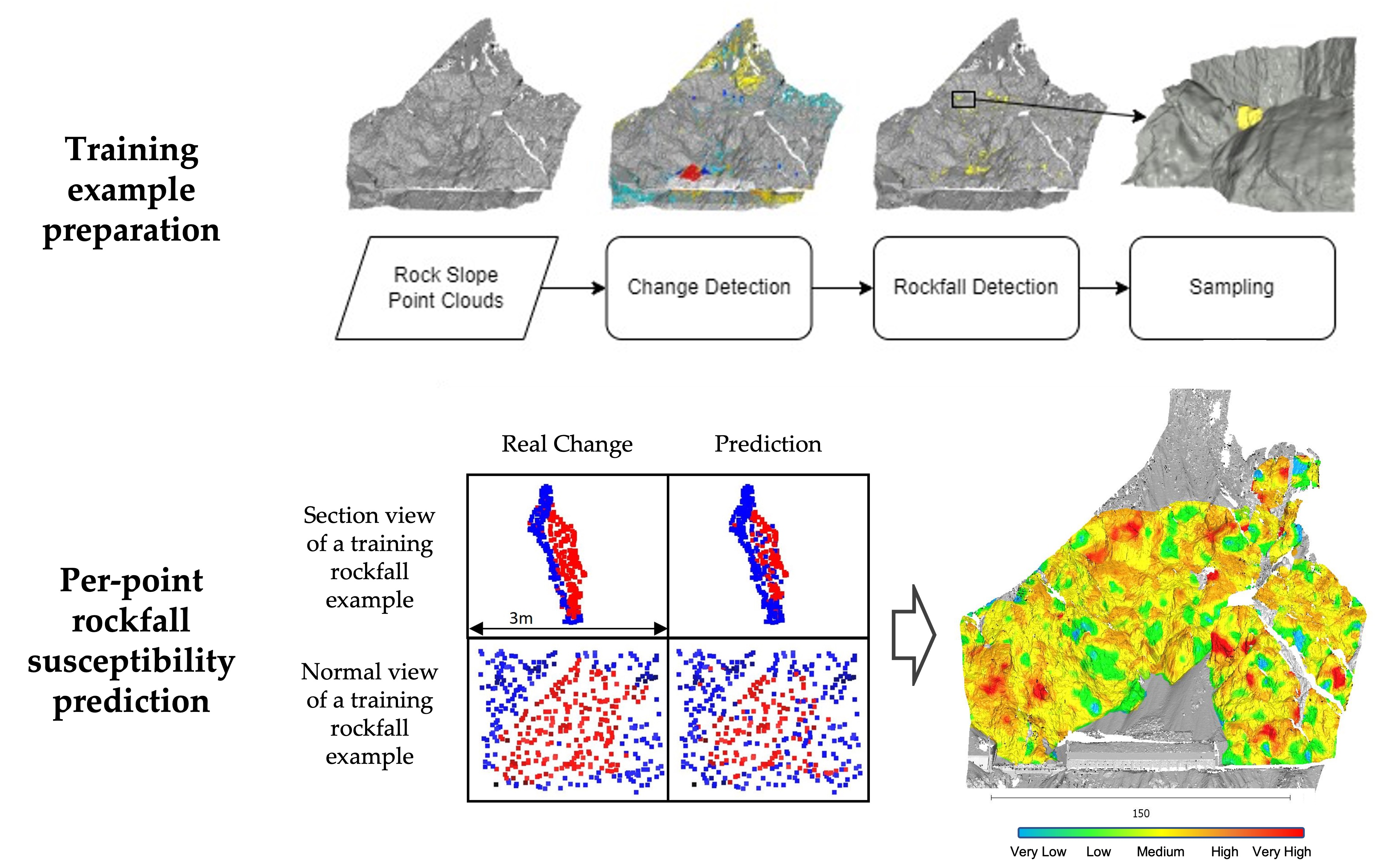
2.1. Conceptualization

Almost all the geometric rockfall-governing parameters can be determined to some degree by expert observations (the human visual system). The depth-perception mechanisms of the human visual system allow human beings to subjectively estimate parameters such as size, elevation, and orientation [31]. For instance, standing across from a rock slope and observing it, an engineering geologist or relevant professional can “see” relative distances among points. According to Gestalt’s theory [32] and the human visual system’s predisposition to group sets of elements, the expert can therefore identify the relative orientation, size, and roughness of surfaces, the relative distance between surfaces, and areas that are closer to the viewpoint than their surroundings (critical overhanging blocks).

The above-mentioned mechanism of making observations, coupled with the human brain’s (biological neural networks) ability to explore patterns in sets of observations of a certain matter, generates knowledge through experience. This process is what has eventually led to the development of engineering geological knowledge expressed by means of concepts such as discontinuity sets and kinematic analysis (relative orientations), joint spacing and persistence (relative distances), weathering degree (relative color), and, in fact, all the aforementioned morphological attributes. Therefore, provided that an expert is able to continuously observe and memorize over the long term the evolution of a rock slope and discover correlations with their knowledge, data-driven RSM could be described as a vision problem. However, even in this theoretical case, biological limitations such as memory capacity would disfavor the expert’s attempts to assess rockfall susceptibility.

To bypass these limitations, the current study explores the potential of simulating slope-scale RSM using computer power and Artificial Intelligence (AI). CV utilizes DL, which is the subfield of Machine Learning (ML) that aims at learning from data using human brain simulations. It is achieved by employing structures and algorithms known as Artificial Neural Networks (ANNs), inspired by the function of the human brain. Specifically, different point cloud semantic segmentation (PCSS) neural networks are employed to model rockfall susceptibility. Semantic segmentation has been a fundamental research challenge in the field of CV and refers to the process of assigning a semantic label to each pixel of an image. PCSS, instead, which is the 3D form of semantic segmentation, is defined as the per-point semantic labeling of a point cloud in 3D space. However, despite being widely used in recent DL applications in CV, PCSS is usually called “point cloud classification” in RS, generating confusion between the two terms [33].

The process includes three main steps, as illustrated in Figure 1, which describe the whole workflow from sequential LiDAR scanning to the evaluation of different DL models for rockfall susceptibility modeling at slope scale. Firstly, the sequential point cloud datasets are pre-processed to create the input training examples. Change detection is performed between successive scans, and rockfall training examples are collected according to the strategy described in the data preparation Section 2.3. Furthermore, the DL architecture, the loss function, and the optimization algorithm are defined. Finally, the training examples are iteratively used to train, validate, and test the neural networks after being partitioned into the respective splits. The performance during the testing phase is evaluated based on various metrics over the test split.

In ML, knowledge is expressed by means of features (attributes). Features can be either handcrafted or learned. In contrast to traditional ML classifiers, DL does not require feature engineering (existing knowledge representation), but rather seeks to exploit the unknown structure in the input data distribution in order to discover good representations (form its own experience/knowledge) [34]. As such, in our approach, the human vision system input equivalent to the ANNs is expressed by: (a) XYZ coordinates (position, distance, elevation, size perception, etc.) and (b) normal vectors (orientation perception), as well as (c) the labeling of the blocks that have eventually failed (Figure 2). Unfortunately, color values that could assist in generating knowledge about lithology and/or weathering were not available in the examined databases. Nevertheless, the above input comprises the required initial visual signal to generate morphological and structural knowledge.

2.2. Study Areas and Datasets

The research is conducted based on three large LiDAR-based monitoring databases of geomorphologically distinct rock slopes in British Columbia, Canada, and the northeast UK (Figure 3).

2.2.1. Mile 109

The CN Rail Ashcroft Mile 109.4 site (Figure 4), known as Mile 109, is an engineered rock slope located along the Frazer River in British Columbia, Canada. This rock slope is 240 m long, runs parallel to the CN track, and is approximately 65 m high. It is composed of successive layers of argillites, sandy siltstones, shales, sandstones, and conglomerates. Normal faults and shear zones cut the sedimentary layers along the slopes, creating favorable conditions for rockfalls. More details about the geologic setting and the failure patterns and mechanisms can be found in [30,35].

The rockfall database utilized in this study resulted from a 5-year-long monitoring program that was initiated after intense rockfall activity caused severe problems for the underlying infrastructure. It includes 24 instances of the rock slope with a point spacing of 5 cm acquired periodically between 2013 and 2018 and more than 3400 recorded rockfall events of varying magnitude and shape [35].

2.2.2. White Canyon West

The second rockfall database comes from the west part of the White Canyon (WCW) (Figure 5) in British Columbia, Canada. The site is approximately 1000 m long and up to 300 m high, with steep metamorphic rock dykes and large debris channels traversing the slopes. Refs. [36,37] discuss the details of the rockfall activity and the associated debris transfer activity patterns in the White Canyon, respectively.

This database represents a different geological and geomorphological environment from the Mile 109 site that is being monitored as part of the same monitoring program (RGHRP—Railway Ground Hazard Research Program). However, WCW is significantly larger than Mile 109 in size and similarly rockfall-active. The monitoring database includes more than 10,000 recorded rockfall events extracted based on the methods proposed by [35,36,38]. Each data acquisition consists of hundreds of millions of points, with a maximum raw point spacing of 10 cm.

2.2.3. Marsden Bay

The third rockfall database has been derived from the coastal cliffs at Marsden Bay, located just south of the river Tyne in the northeast of England (Figure 6). The focus area is a 740-m coastal stretch comprised of three shallow bays where the close proximity of the eroding cliffs threatens a key road, the A183, that connects the coastal communities of South Shields and Whitburn [39]. The cliffs are approximately 27 m high and expose clear layers of dolomitic limestone, secondary limestone, and areas of breccia [40]. The cliffs are fronted by shore platforms, pocket beaches, and boulder fields in places that refract and dissipate nearshore wave energies. The rockfall database is described in detail in [40] but was generated from 24 terrestrial laser scanning surveys with a resolution of 10 cm captured approximately monthly between February 2015 and March 2017, producing more than 30,000 rockfalls.

2.3. Data Preparation

The raw rock slope point clouds are collected by terrestrial LiDAR scanning (TLS) in high resolution, generating large datasets (several gigabytes) monthly to seasonally. To generate the required inputs for the training of the DL models, the authors implement a three-step data preparation process, including: (a) change detection, (b) rockfall detection, and (c) sampling.

Change detection was carried out between consecutive point clouds. The process includes not only the calculation of distances between the inputs but also noise filtering and spatial clustering, as discussed in [30]. Subsequently, rockfall detection neural networks that have been developed for the sites according to [35] are used to extract rockfall events among clusters that may also correspond to other surficial changes (e.g., talus movement).

Since all the rockfall points associated with each acquisition date are known, it is possible to discreetly sample the data to generate training examples. Due to the prohibitively large GPU memory capacity required and the associated computational cost for the application of DNNs to large and high-resolution (10 cm point spacing) point clouds, smaller-scale snapshots are formed (see the “sampling” step in Figure 1 and Figure 2). Specifically, a fixed-sized bounding box centered at the barycenter of each rockfall cluster is first calculated. Following that, the intersection of the prior-to-failure terrain point cloud with the computed bounding box is cropped out. The goal of this practice is to ensure that, for each rockfall event, the learned features represent not only the local rock slope surface prior to failure but also the “stable” geometry surrounding the rockfall volume. All the points within the cropped area that correspond to the rockfall cluster are labeled with 1 and the rest with 0, forming one training example. Each sample has six channels, indicating $x, y, \mathrm{and} z$ coordinates and $n_x$, $n_y$, and $n_z$ vector values.

The process is repeated four more times, moving the box to locate the rockfall at the four corners, respectively. This leads to five training examples created from each rockfall event. Each one of the training examples contains at least one rockfall cluster (points belonging to detected negative changes) surrounded by “stable” rock (points belonging to areas not deformed between two successive monitoring campaigns). This sampling technique is applied to prevent the neural network from being biased so that a rockfall-susceptible area is more likely to be located at the center of an examined scene.

2.4. Deep Learning Models

Among the multi-view, volumetric-based, and point-based PCSS methods discussed in the literature [41], this study focuses on the most common point-based approaches. These models directly consume the real 3D information and technically define the smallest possible spatial entity (i.e., a point within the overall 3D point cloud) as the mapping unit of this novel approach to RSM. The DL architectures selected for this investigation represent the three types of direct point-based learning. These are: Pointwise Multi-Layer Perceptron (MLP), Point Convolution, and Graph-based methods that are represented by PointNet++ [42], PointCNN [43], and DGCNN [44] models, respectively. These 3D learning architectures, which are utilized to determine their suitability to relate local rock slope geometry with recorded rockfall events, are described in more detail in the subsequent sub-sections.

2.4.1. Pointwise MLP-Based Learning

Based on its ancestor, PointNet [45], PointNet++ is a pioneering hierarchical DL network that utilizes pointwise MLP-based learning. PointNet, as the main building block of PointNet++, models each input point independently with several shared MLPs. In this way, the network learns pointwise features and achieves permutation invariance by aggregating global feature representations using a symmetric function. However, the local structure and interrelationships between points cannot be captured because the point features are learned independently.

To capture the local structure around each point, PointNet++ employs a set abstraction level, including sampling, grouping, and a PointNet-based learning layer. Thus, PointNet++ is able to learn and abstract local feature representations by stacking several sets of abstraction levels together. The development of many networks has been based on PointNet or a PointNet-like architecture due to its robustness.

2.4.2. Point Convolution-Based Learning

In general, due to their unstructured nature and irregularities, it is hard to apply convolutional operations to 3D point clouds. In 2D, the rigid grid structure of image datasets favors the design of convolutional kernels, but in 3D, this has been a rather challenging operation to implement. PointCNN achieves hierarchical representation learning by generalizing the hierarchical application of convolutions to point clouds. The network employs an X-Conv transformation to realize equivariance and address the information loss problem of pooling in achieving permutation invariance. The input points are thus transformed into a canonical order, and typical convolutional operations can be subsequently applied to the transformed features. The structure and form of the inputs for PointCNN can be seen below.

PointCNN input $F_1=\left\{\left(p_{1,i}, f_{1,i}\right):i=1, 2, \dots , N_1\right\}$, is a set of points $\left\{p_{1,i}:p_{1,i}\in {ℝ}^{Dim}\right\}$, each associated with a feature $\left\{f_{1,i}:f_{1,i}\in {ℝ}^{C_1}\right\}$. The X-Conv operation is applied on $F_1$ to obtain higher-level representation $F_2=\left\{\left(p_{2,i}, f_{2,i}\right):f_{2,i}\in {ℝ}^{C_2}, i=1, 2, \dots , N_2\right\}$, where $\left\{p_{2,i}\right\}$ is a set of representative points of $\left\{p_{1,i}\right\}$ and $F_2$ is of coarser spatial resolution and deeper feature representation than $F_1$ (i.e., $N_2<N_1$ and $C_2>C_1$). The above process is applied hierarchically, following the typical structure of grid-based convolutional neural networks (CNNs).

2.4.3. Graph-Based Learning

In graph-based learning, each point of the input point cloud ${\rm X}=\left(x_1, \dots ,x_n\right)\subseteq {ℝ}^{Dim}$ is considered a vertex of a graph representation. Directed edges are generated for a set of neighboring vertices, modeling the spatial relationships among the points. Such methods define convolution operations in the spatial domain. Several MLPs are usually employed over spatial neighbors, and successively coarser graph representations are produced by feature aggregation through the pooling of layers.

DGCNN constructs a directed graph representation $G=\left(V, E\right)$ in the feature space, where $V=\left\{1,\dots , n\right\}$ and $E\subseteq V\times V$ are vertices and edges, respectively, and is dynamically updated at each layer. To capture the local geometric structure while maintaining permutation invariance, DGCNN introduces the EdgeConv layer as its core operation. With EdgeConv, the network computes features at the edges of the graph at each layer to characterize the relationships between a point and its neighbors as $e_{ij}=h_{\theta }\left(x_i, x_j\right)$, where $h_{\theta }:{ℝ}^{Dim}\times {ℝ}^{Dim}\to {ℝ}^{Di{m}^{’}}$ is a nonlinear function with a set of learnable parameters $\theta$. Since EdgeConv explicitly constructs a local graph and learns the embeddings for the edges, DGCNN can group points in both Euclidean and semantic space.

2.5. Model Development and Evaluation

To maintain consistency in the analyses and comparisons of the different models, the same training strategy is applied to all the models. The whole sets of training examples for each use case are split into training (70%), development (15%), and test sets (15%). Hyperparameter tuning is carried out using a grid-search approach. The implementation of all the models is based on the Tensorflow 2 framework. The trainable parameters of the models are optimized by minimizing the binary cross-entropy (BCE) loss based on the ground truth datasets and the predicted probabilities on the training set. The performance on the development set is used to tune the models’ hyperparameters. The Adam optimizer is used to minimize the BCE loss during training as follows:

$$BC{E}_{Loss}=-\frac{1}{n}{\displaystyle \sum }_{k=1}^n\frac{1}{w\times h}{\displaystyle \sum }_{i=1}^h{\displaystyle \sum }_{j=1}^w{y}_{k,i,j}log\left({\widehat{y}}_{k,i,j}\right)+\left(1-y_{k,i,j}\right) log\left(1-{\widehat{y}}_{k,i,j}\right)$$

(1)

where, $n$ refers to the number of training examples, $y$ to the target labels, and $\widehat{y}$ to the neural network predictions.

The trained models are used to predict either a rockfall or a non-rockfall label for each point in the unseen examples of the test dataset. The semantic segmentation result is evaluated in terms of CV by four metrics, namely: intersection over union (IoU), $F_1$-score, precision, and recall, as well as by calculating the receiver operating characteristic curve (ROC curve) and the area under the curve (AUC), which comprise a typical evaluation approach in landslide susceptibility modeling literature.

Since PCSS neural networks perform per-point classification, there is an absolute correspondence between input (ground truth) and output (predicted) point label vectors. The first four metrics are calculated based on the confusion matrices and the relationships among true positives (TP), true negatives (TN), false positives (FP), and false negatives (FN). Specifically, the receiver operating characteristic (ROC) curve is calculated as a plot between TP and FP rates at various threshold settings. The ROC curve illustrates the diagnostic ability of a binary classifier and is widely used in natural hazard modeling. TP and FP rates are calculated using the following formulas:

$$TP rate \left(recall\right)=\frac{TP}{TP+FN}$$

(2)

$$FP rate=\frac{FP}{FP+TN}$$

(3)

Precision, recall, and F₁-score are also used separately to represent the ability of a model to avoid FPs, the ability to predict positive instances, and a harmonic mean of precision and recall, respectively.

$$Precision=\frac{TP}{TP+FP}$$

(4)

$$F_1-score=\frac{2TP}{2TP+FP+FN}$$

(5)

The fifth metric used is the mean intersection over union (IoU). The IoU is a typical method for the evaluation of semantic segmentation and object detection results. It is used to quantify the mean percent overlap between the ground truth dataset and the prediction result for each class according to the following formula:

$$IoU=\frac{ground truth\cap prediction}{ground truth\cup prediction}$$

(6)

3. Results

This section discusses the results of the experiments that are conducted as part of this investigation in order to determine the potential of a novel CV-based approach to RSM. The effectiveness of three common PCSS DNNs is evaluated by the application of these (PointNet++, PointCNN, and DGCNN) on three LiDAR-based rockfall monitoring databases from Canada and the United Kingdom.

3.1. Quantitative Assessment

The ability of each of the three different PCSS methods to deal with the RSM problem is evaluated based on the test set of each site (Mile 109, WCW, and Marsden). After 100 epochs of training, the weights of the best-performing model on the development set were used to predict rockfall susceptibility in the latest states of each database that composes the test sets. The performance of each model is assessed by means of the five selected metrics shown in

Table 1. Quantitative experimental results of the examined DL architectures on the three test sites.

Model	Dataset	AUC	Precision	Recall	${\mathit{F}}_1-\mathbf{Score}$	IoU
PointNet++	Mile 109	0.75	0.74	0.74	0.74	0.51
	WCW	0.63	0.69	0.89	0.78	0.39
	Marsden	0.62	0.57	0.25	0.35	0.40
PointCNN	Mile 109	0.68	0.69	0.80	0.74	0.46
	WCW	0.66	0.71	0.88	0.79	0.43
	Marsden	0.70	0.60	0.50	0.54	0.48
DGCNN	Mile 109	0.64	0.67	0.80	0.73	0.44
	WCW	0.62	0.69	0.93	0.79	0.37
	Marsden	0.58	0.45	0.10	0.17	0.33

, with the highest scores on each metric highlighted.

PointNet++ and PointCNN produce the best results on all three case sites. Specifically, while PointNet++ achieves the highest overall AUC, precision, and IoU (0.75, 0.74, and 0.51, respectively) on Mile 109, PointCNN slightly outperforms at both WCW and Marsden sites. The latter also achieves the highest overall F1-score (0.79) and the greatest confidence in making predictions for WCW and Marsden. DGCNN appears to be the weakest of the three DL architectures, with a maximum AUC of 0.64 in Mile 109 and 0.58 in Marsden. Overall, it is important to note that the best metric values are consistently achieved for Mile 109 and that PointNet++ is the most promising architecture for RSM at this scale.

Further observation of the ROC curves of the trained models for each case’s test dataset in Figure 7, validates the superiority of PointNet++ compared to the two other DL methods at the Mile 109 site, especially in the lower FP and TP rates. The ROC graphs also reveal the relative stability of the PointCNN models, which consistently maintain an arch-like curve shape in contrast to the slight fluctuations of the PointCNN and DGCNN models. PointCNN also shows relatively good learning behavior, while DGCNN seems to be the least performing 3D DL architecture given the available data at the time. There is a general pattern of PointCNN learning more useful information to relate to rockfall activity and perform site-specific RSM at different settings, with prediction confidence ranging between 66% and 70%.

To further assess the learning process, its improvement, and the potential of this novel approach to RSM, the predictive capabilities are analyzed using different time frames in the database. The Mile 109 database is divided into 12-month intervals and assessed seasonally. As such, a year is defined as the period between the 1st of November and the 31st of October of the next calendar year, starting from 2013 to 2018. The Mile 109 site was selected due to the highest scores that are achieved for this site as well as the relatively even rockfall frequency between epochs. The five fractions are passed into the three models successively, and the predictions are evaluated based on the standard test dataset. By generating and using additional training examples from rockfall monitoring campaigns every year, the ability of the models to cope with RSM increases for all the models and particularly for PointNet++, which presents an almost 14% improvement throughout the first 4 years of training data (Figure 8).

3.2. Site-Specific RSM Application

The different DL models have been applied to the entire rock slope’s 3D point clouds for RSM. Figure 9, Figure 10 and Figure 11 illustrate rockfall susceptibility in block-level spatial resolution for Mile 109, WCW, and Marsden sites, respectively. The maps are produced by visualizing the probability of each point in the point cloud belonging to the positive instance of the binary per-point classification (i.e., rockfall class). The output is categorized into five equal rockfall susceptibility classes.

The models have been trained with individually formed training examples. This in fact means that internal characteristics are learned for each training example (see Section 2.3) without any spatial relationship among them. Thus, to make predictions about an unseen scene, local samples need to be iteratively collected and their points labeled separately. However, even though spatial relationships among the training examples are not maintained or learned, it is promising and impressive that the predicted values are spatially grouped within the maps. This indicates both the correlation of local geometry with rockfall activity and the potential to keep on learning useful features and increase performance with the amount and quality of training examples.

3.2.1. Mile 109

The Mile 109 site is a typical tectonized sedimentary environment with steep and sharp rock sections as well as benches and smoother areas formed by bedding and tectonic discontinuity planes. In this setting, the majority of the failures are sourced from the steeper sections, spires, and overhanging blocks. In general, all models tend to predict that most of the steep parts of the slope are more susceptible to rockfall (Figure 9). The rockfall susceptibility maps produced by PointNet++ and PointCNN are similar except that PointCNN evaluates the “high” susceptibility areas of PointNet++ as “very high”. Both architectures are able to clearly differentiate between steep and sharp regions across the whole slope, placing them within the “high” and “very high” classes. In contrast, DGCNN neglects large, “low”-class areas along the crown of the slope that are known to have generated intense rockfall activity in the past years [30,35].

3.2.2. White Canyon West

In the WCW case, the majority of the rockfall activity is sourced from the steep sections just above the long debris channels that traverse the slopes [35,36,37]. The rockfall susceptibility maps of the three DL models are presented in Figure 10. As reflected by the AUC values, PointCNN’s map seems to better separate the sections surrounding the channels as having “high” susceptibility and the rest of the slope as having “low” susceptibility. PointNet++, on the other hand, does not “see” significant variations of the rockfall susceptibility along the slope, rating almost its entire extent as “medium” susceptibility and only a few steep sections as “high”, without any “very high” parts as expected given the experience and knowledge about the site. In general, PointNet++ susceptibility values range between 46% and 62%. This demonstrates that either the data are not sufficient for PointNet++ to develop a perception of this site, or this learning algorithm is not the most suitable for this case. However, it requires further investigation with perhaps more data to confidently provide definitive conclusions. Lastly, although DGCNN is not the best-performing model in terms of AUC, it seems to “understand” a realistic rockfall susceptibility pattern for this site. Specifically, apart from the steep areas around the channels, DGCNN values “high” to “very high” susceptibility areas in the lower part of the slope at the track level. Those areas are steep outcrops up to 20 m high at the middle and left parts (face on view) of WCW that have sourced numerous rockfall events in the past [36].

3.2.3. Marsden Bay

In Marsden Bay, as a typically bedded sedimentary outcrop, most of the rockfall events are aligned horizontally, mainly on the top of the cliffs, as well as in some sharp areas in the middle and other parts of the site. Our experiments show that PointCNN is able to better separate these areas, suggesting a thin “high” susceptibility top layer and large “low” to “very low” sections in the middle and lower parts (Figure 11). This is a typical illustration of the activity taking place in the area, which includes wave erosion leading to overhanging blocks that eventually fail. Neither PointNet++ nor DGCNN seem to generate a similar understanding of the patterns, which is also evident by the AUC scores in Figure 7.

4. Discussion

This paper presents the results of a new DL-based approach to RSM. Slope-scale RSM is approached as a 3D computer vision problem based on high-resolution LiDAR data, with the goal of improving the accuracy of the predictions. Traditionally, data-driven RSM is conducted at regional scales based on slope units over 2.5D (rasterized) terrain models. We leverage computer power and AI to learn from the experience of a rock slope through digital observations of its evolution. Our approach endeavors to predict future rockfall source areas by means of individual rock blocks, considering individual 3D points as mapping units. This would benefit modern sophisticated physics engine-based rockfall simulations to realistically and more accurately assess rockfall hazards.

We used three different digital 3D rockfall databases with different characteristics to test our hypothesis. The results indicate strong potential to achieve AI development with engineering and geological perception of local geometry as a controlling factor of rockfall activity. Moreover, the experiments revealed a clear indication of learning with experience (seeing more examples) (Figure 8). The continuous improvement of AUC scores indicates that the predictions approach RSM reasonably and encourages the further establishment of such monitoring programs and the collection of more training data. Change detection between systematically acquired LiDAR scans generates high-quality annotated point clouds for the training phase.

We believe that with the current advances in sensors and DL, data-driven approaches based on sound data collection strategies can lead the evolution of rock slope management practices. To date, geometry has been mainly used to represent local rock mass structure, but the addition of color might provide knowledge regarding rock types, weathering, and moisture to better explain rockfall activity patterns. Furthermore, this type of knowledge representation can be extended to more DL approaches other than semantic segmentation. For instance, based on the presented results of 3D learning on rock slopes, future research is encouraged to consider sequence modeling. The analysis of dynamic sequences, such as sequential rockfall instances, could also assist in modeling the temporal aspect of rock slope evolution and produce slope-scale hazard modeling for spatiotemporal predictions.

5. Conclusions

The models are able to produce slope-scale rockfall susceptibility maps in high resolution with an AUC up to 0.75 (Figure 7). The approach employs PCSS methods, which perform per-point prediction. In this regard, it is impressive that points of similar rockfall susceptibility values are spatially grouped along the examined slopes (Figure 9, Figure 10 and Figure 11), even though spatial relationships are neither maintained nor learned. It shows that treating RSM as a vision problem enables AI-based, data-driven RSM at very high resolution. Our results imply that the DL models are able to develop a perception of rock slope geometry and the location of critical blocks, thereby imitating a field expert who deterministically assesses rockfall susceptibility in a qualitative manner based on their knowledge and experience but perhaps lacks empirical data to inform their analysis. In general, point convolution-based learning poses steady learning behavior and maintains gradual improvement with experience. Pointwise MLP-based and graph-based learning show variations at the different sites, with the former achieving a higher and the latter a lower AUC.

In conclusion, spatially accurate data-driven slope-scale RSM predictions can be achieved for individual rock slope systems. The proposed framework for encoding engineering geological observations throughout a rock slope’s evolution is proven to comprise a critical advance towards learning geoengineering concepts from data. This research encourages building on the proposed methodology to leverage computer power and artificial intelligence. However, confidence levels are still relatively low at the moment. Future research should not only focus on the incorporation of more training examples but also consider color values as additional raw information as well as proper data collection for sequence modeling purposes, with the goal of accounting for both spatial and temporal rockfall patterns at the same time.

References

1. Hungr, O.; Leroueil, S.; Picarelli, L. The Varnes Classification of Landslide Types, an Update. Landslides 2014, 11, 167–194. [Google Scholar] [CrossRef]
2. Guzzetti, F.; Reichenbach, P.; Cardinali, M.; Galli, M.; Ardizzone, F. Probabilistic Landslide Hazard Assessment at the Basin Scale. Geomorphology 2005, 72, 272–299. [Google Scholar] [CrossRef]
3. Reichenbach, P.; Rossi, M.; Malamud, B.D.; Mihir, M.; Guzzetti, F. A Review of Statistically-Based Landslide Susceptibility Models. Earth Sci. Rev. 2018, 180, 60–91. [Google Scholar] [CrossRef]
4. Guzzetti, F.; Crosta, G.; Detti, R.; Agliardi, F. STONE: A Computer Program for the Three-Dimensional Simulation of Rock-Falls. Comput. Geosci. 2002, 28, 1079–1093. [Google Scholar] [CrossRef]
5. Gallo, I.G.; Martínez-Corbella, M.; Sarro, R.; Iovine, G.; López-Vinielles, J.; Hérnandez, M.; Robustelli, G.; Mateos, R.M.; García-Davalillo, J.C. An Integration of Uav-Based Photogrammetry and 3D Modelling for Rockfall Hazard Assessment: The Cárcavos Case in 2018 (Spain). Remote Sens. 2021, 13, 3450. [Google Scholar] [CrossRef]
6. Agliardi, F.; Crosta, G.B. High Resolution Three-Dimensional Numerical Modelling of Rockfalls. Int. J. Rock Mech. Min. Sci. 2003, 40, 455–471. [Google Scholar] [CrossRef]
7. Alvioli, M.; Santangelo, M.; Fiorucci, F.; Cardinali, M.; Marchesini, I.; Reichenbach, P.; Rossi, M.; Guzzetti, F.; Peruccacci, S. Rockfall Susceptibility and Network-Ranked Susceptibility along the Italian Railway. Eng. Geol. 2021, 293, 106301. [Google Scholar] [CrossRef]
8. Samodra, G.; Chen, G.; Sartohadi, J.; Hadmoko, D.S.; Kasama, K.; Setiawan, M.A. Rockfall Susceptibility Zoning Based on Back Analysis of Rockfall Deposit Inventory in Gunung Kelir, Java. Landslides 2016, 13, 805–819. [Google Scholar] [CrossRef]
9. Fell, R.; Corominas, J.; Bonnard, C.; Cascini, L.; Leroi, E.; Savage, W.Z. Guidelines for Landslide Susceptibility, Hazard and Risk Zoning for Land-Use Planning. Eng. Geol. 2008, 102, 99–111. [Google Scholar] [CrossRef]
10. Corominas, J.; Copons, R.; Moya, J.; Vilaplana, J.M.; Altimir, J.; Amigó, J. Quantitative Assessment of the Residual Risk in a Rockfall Protected Area. Landslides 2005, 2, 343–357. [Google Scholar] [CrossRef]
11. Guzzetti, F.; Carrara, A.; Cardinali, M.; Reichenbach, P. Landslide hazard evaluation: A review of current techniques and their application in a multi-scale study, Central Italy. Geomorphology 1999, 31, 181–216. [Google Scholar] [CrossRef]
12. Hungr, O.; Evans, S.G.; Hazzard, J. Magnitude and Frequency of Rock Falls and Rock Slides along the Main Transportation Corridors of Southwestern British Columbia. Can. Geotech. J. 1999, 36, 224–238. [Google Scholar] [CrossRef]
13. Lombardo, L.; Tanyas, H.; Huser, R.; Guzzetti, F.; Castro-Camilo, D. Landslide Size Matters: A New Data-Driven, Spatial Prototype. Eng. Geol. 2021, 293, 106288. [Google Scholar] [CrossRef]
14. Farmakis, I.; Marinos, V.; Papathanassiou, G.; Karantanellis, E. Automated 3D Jointed Rock Mass Structural Analysis and Characterization Using LiDAR Terrestrial Laser Scanner for Rockfall Susceptibility Assessment: Perissa Area Case (Santorini). Geotech. Geol. Eng. 2020, 38, 3007–3024. [Google Scholar] [CrossRef]
15. Wichmann, V.; Strauhal, T.; Fey, C.; Perzlmaier, S. Derivation of Space-Resolved Normal Joint Spacing and in Situ Block Size Distribution Data from Terrestrial LIDAR Point Clouds in a Rugged Alpine Relief (Kühtai, Austria). Bull. Eng. Geol. Environ. 2019, 78, 4465–4478. [Google Scholar] [CrossRef]
16. Lato, M.; Diederichs, M.S.; Hutchinson, D.J.; Harrap, R. Optimization of LiDAR Scanning and Processing for Automated Structural Evaluation of Discontinuities in Rockmasses. Int. J. Rock Mech. Min. Sci. 2009, 46, 194–199. [Google Scholar] [CrossRef]
17. Jaboyedoff, M.; Oppikofer, T.; Abellán, A.; Derron, M.H.; Loye, A.; Metzger, R.; Pedrazzini, A. Use of LIDAR in Landslide Investigations: A Review. Nat. Hazards 2012, 61, 5–28. [Google Scholar] [CrossRef]
18. Westoby, M.J.; Brasington, J.; Glasser, N.F.; Hambrey, M.J.; Reynolds, J.M. “Structure-from-Motion” Photogrammetry: A Low-Cost, Effective Tool for Geoscience Applications. Geomorphology 2012, 179, 300–314. [Google Scholar] [CrossRef]
19. Cirillo, D.; Cerritelli, F.; Agostini, S.; Bello, S.; Lavecchia, G.; Brozzetti, F. Integrating Post-Processing Kinematic (PPK)–Structure-from-Motion (SfM) with Unmanned Aerial Vehicle (UAV) Photogrammetry and Digital Field Mapping for Structural Geological Analysis. ISPRS Int. J. Geo-Inf. 2022, 11, 437. [Google Scholar] [CrossRef]
20. van Westen, C.J.; Castellanos, E.; Kuriakose, S.L. Spatial Data for Landslide Susceptibility, Hazard, and Vulnerability Assessment: An Overview. Eng. Geol. 2008, 102, 112–131. [Google Scholar] [CrossRef]
21. Amato, G.; Eisank, C.; Castro-Camilo, D.; Lombardo, L. Accounting for Covariate Distributions in Slope-Unit-Based Landslide Susceptibility Models. A Case Study in the Alpine Environment. Eng. Geol. 2019, 260, 105237. [Google Scholar] [CrossRef]
22. Gudiyangada Nachappa, T.; Kienberger, S.; Meena, S.R.; Hölbling, D.; Blaschke, T. Comparison and Validation of Per-Pixel and Object-Based Approaches for Landslide Susceptibility Mapping. Geomat. Nat. Hazards Risk 2020, 11, 572–600. [Google Scholar] [CrossRef]
23. Shirzadi, A.; Saro, L.; Hyun Joo, O.; Chapi, K. A GIS-Based Logistic Regression Model in Rock-Fall Susceptibility Mapping along a Mountainous Road: Salavat Abad Case Study, Kurdistan, Iran. Nat. Hazards 2012, 64, 1639–1656. [Google Scholar] [CrossRef]
24. Cignetti, M.; Godone, D.; Bertolo, D.; Paganone, M.; Thuegaz, P.; Giordan, D. Rockfall Susceptibility along the Regional Road Network of Aosta Valley Region (Northwestern Italy). J. Maps 2021, 17, 54–64. [Google Scholar] [CrossRef]
25. Losasso, L.; Sdao, F. The Artificial Neural Network for the Rockfall Susceptibility Assessment: A Case Study in Basilicata (Southern Italy). Geomat. Nat. Hazards Risk 2018, 9, 737–759. [Google Scholar] [CrossRef]
26. Du, B.; Zhao, Z.; Hu, X.; Wu, G.; Han, L.; Sun, L.; Gao, Q. Landslide Susceptibility Prediction Based on Image Semantic Segmentation. Comput. Geosci. 2021, 155, 104860. [Google Scholar] [CrossRef]
27. Ji, S.; Yu, D.; Shen, C.; Li, W.; Xu, Q. Landslide Detection from an Open Satellite Imagery and Digital Elevation Model Dataset Using Attention Boosted Convolutional Neural Networks. Landslides 2020, 17, 1337–1352. [Google Scholar] [CrossRef]
28. Sala, Z.; Jean Hutchinson, D.; Harrap, R. Simulation of Fragmental Rockfalls Detected Using Terrestrial Laser Scans from Rock Slopes in South-Central British Columbia, Canada. Nat. Hazards Earth Syst. Sci. 2019, 19, 2385–2404. [Google Scholar] [CrossRef]
29. Harrap, R.M.; Hutchinson, D.J.; Sala, Z.; Ondercin, M.; Difrancesco, P.M. Our GIS Is a Game Engine: Bringing Unity to Spatial Simulation of Rockfalls. In Proceedings of the GeoComputation 2019, Queenstown, New Zealand, 18–21 September 2019. [Google Scholar]
30. DiFrancesco, P.M.; Bonneau, D.; Hutchinson, D.J. The Implications of M3C2 Projection Diameter on 3D Semi-Automated Rockfall Extraction from Sequential Terrestrial Laser Scanning Point Clouds. Remote Sens. 2020, 12, 1885. [Google Scholar] [CrossRef]
31. Howard, I.P. Perceiving in DepthVolume 3 Other Mechanisms of Depth Perception; Oxford University Press: Oxford, UK, 2012; ISBN 9780199764167. [Google Scholar]
32. Koffka, K. Principles of Gestalt Psychology; Routledge: London, UK, 2013; ISBN 9781136306815. [Google Scholar]
33. Xie, Y.; Tian, J.; Zhu, X.X. Linking Points with Labels in 3D: A Review of Point Cloud Semantic Segmentation. IEEE Geosci. Remote Sens. Mag. 2020, 8, 38–59. [Google Scholar] [CrossRef]
34. Bengio, J. Deep Learning of Representations for Unsupervised and Transfer Learning. ICML Unsupervised Transf. Learn. 2012, 27, 17–36. [Google Scholar]
35. Farmakis, I.; DiFrancesco, P.M.; Hutchinson, D.J.; Vlachopoulos, N. Rockfall Detection Using LiDAR and Deep Learning. Eng. Geol. 2022, 309, 106836. [Google Scholar] [CrossRef]
36. Kromer, R.A.; Hutchinson, D.J.; Lato, M.J.; Gauthier, D.; Edwards, T. Identifying Rock Slope Failure Precursors Using LiDAR for Transportation Corridor Hazard Management. Eng. Geol. 2015, 195, 93–103. [Google Scholar] [CrossRef]
37. Bonneau, D.A.; Hutchinson, D.J.; McDougall, S. Characterizing Debris Transfer Patterns in the White Canyon, British Columbia with Terrestrial Laser Scanning. In Proceedings of the 7th International Conference on Debris-Flow Hazards Mitigation: Mechanics, Monitoring, Modeling, and Assessment, Golden, CO, USA, 10–13 June 2019; pp. 565–572. [Google Scholar]
38. van Veen, M.; Hutchinson, D.J.; Kromer, R.; Lato, M.; Edwards, T. Effects of Sampling Interval on the Frequency-Magnitude Relationship of Rockfalls Detected from Terrestrial Laser Scanning Using Semi-Automated Methods. Landslides 2017, 14, 1579–1592. [Google Scholar] [CrossRef]
39. Westoby, M.J.; Lim, M.; Hogg, M.; Pound, M.J.; Dunlop, L.; Woodward, J. Cost-Effective Erosion Monitoring of Coastal Cliffs. Coast. Eng. 2018, 138, 152–164. [Google Scholar] [CrossRef]
40. Westoby, M.; Lim, M.; Hogg, M.; Dunlop, L.; Pound, M.; Strzelecki, M.; Woodward, J. Decoding Complex Erosion Responses for the Mitigation of Coastal Rockfall Hazards Using Repeat Terrestrial LiDAR. Remote Sens. 2020, 12, 2620. [Google Scholar] [CrossRef]
41. Guo, Y.; Wang, H.; Hu, Q.; Liu, H.; Liu, L.; Bennamoun, M. Deep Learning for 3D Point Clouds: A Survey. IEEE Trans. Pattern Anal. Mach. Intell. 2021, 43, 4338–4364. [Google Scholar] [CrossRef]
42. Qi, C.; Yi, L.; Su, H.; Guibas, L. PointNet++: Deep Hierarchical Feature Learning on Point Sets in a Metric Space. In Proceedings of the NIPS’17—31st International Conference on Neural Information Processing Systems, Long Beach, CA, USA, 4–9 December 2017; pp. 5105–5114. [Google Scholar]
43. Li, Y.; Bu, R.; Sun, M.; Wu, W.; Di, X.; Chen, B. PointCNN: Convolution on X-Transformed Points. In Proceedings of the Advances in Neural Information Processing Systems (NeurIPS 2018), Montreal, QC, Canada, 3–8 December 2018; pp. 820–830. [Google Scholar]
44. Wang, Y.; Sun, Y.; Liu, Z.; Sarma, S.E.; Bronstein, M.M.; Solomon, J.M. Dynamic Graph CNN for Learning on Point Clouds. ACM Trans. Graph. 2019, 38, 146. [Google Scholar] [CrossRef]
45. Qi, C.R.; Su, H.; Mo, K.; Guibas, L.J. PointNet: Deep Learning on Point Sets for 3D Classification and Segmentation. In Proceedings of the 30th IEEE Conference on Computer Vision and Pattern Recognition, CVPR 2017, Honolulu, HI, USA, 21–26 July 2017; pp. 77–85. [Google Scholar]
Figure 1. Chart demonstrating the entire point cloud semantic segmentation-based workflow for rockfall susceptibility modeling at slope scale. The workflow is divided into three parts: (i) Data preparation: including the steps from change detection to the formation of rockfall training examples; (ii) Model building: including the ML engineering procedures from data split to the compilation of different models; and (iii) Development and evaluation: including the optimization of the models as well as the quantitative and qualitative assessment of the results.
Remotesensing 15 02712 g001
Figure 2. An example of the input to the proposed rockfall susceptibility approach where the local geometry has led to the failure of a wedge. (a) point cloud of the geometry prior to failure (enabling perception of position, distance, elevation, and size); (b) point cloud with normals overlain as black arrows (adds orientation perception to build understanding of the local structure, such as the surfaces that form the wedge); and (c) point cloud with normals and labeled wedge points in yellow (to create correlations between the local geometry and the target “object”).
Remotesensing 15 02712 g002
Figure 3. Location map of the study areas as blue dots: (A) Mile 109, (B) White Canyon West, and (C) Marsden Bay.
Remotesensing 15 02712 g003
Figure 4. View of the CN Rail Ashcroft Mile 109.4 rock slope.
Remotesensing 15 02712 g004
Figure 5. View of a section of the White Canyon West, indicative of its complex geomorphology.
Remotesensing 15 02712 g005
Figure 6. Oblique view of Permian Magnesian Limestone cliffs at the southern end of Marsden Bay, South Shields, UK.
Remotesensing 15 02712 g006
Figure 7. ROC curve graphs of DL-based RSM for Mile 109, WCW and Marsden Bay.
Remotesensing 15 02712 g007
Figure 8. Learning progress of PointNet++, PointCNN, and DGCNN models with successively added annual training data from the Mile 109 database.
Remotesensing 15 02712 g008
Figure 9. High-resolution AI-based rockfall susceptibility maps of Mile 109 with (a) PointNet++, (b) PointCNN, and (c) DGCNN neural networks.
Remotesensing 15 02712 g009
Figure 10. High-resolution AI-based rockfall susceptibility maps of WCW with (a) PointNet++, (b) PointCNN, and (c) DGCNN neural networks.
Remotesensing 15 02712 g010
Figure 11. High-resolution AI-based rockfall susceptibility maps of Marsden Bay with (a) PointNet++, (b) PointCNN, and (c) DGCNN neural networks.
Remotesensing 15 02712 g011