Spatiotemporal Analysis and Multi-Scenario Prediction of Ecosystem Services Based on Land Use/Cover Change in a Mountain-Watershed Region, China

Abstract

Land use/cover change (LUCC) accompanied by climate change and human activities will have unpredictable impacts on watershed ecosystems. However, the extent to which these land use changes affect the spatial and temporal distribution of ecosystem services (ESs) in different regions remains unclear. The impact of LUCC on ESs in the Qingjiang Watershed (QJW), an ecologically sensitive area, and LUCC’s role in future ESs under different land use scenarios are crucial to promoting ecological conservation and land use management. This paper assessed water yield (WY), soil conservation (SC), carbon storage (CS) and habitat quality (HQ) using the InVEST model, and their responses to LUCC in the QJW from 1990 to 2018 using the geodetector and multiscale geographically weighted regression. We predicted land use patterns using the Logistic–CA–Markov model and their effects on ESs in 2034 under business as usual (BAU), ecological land protection (ELP), arable land protection (ALP) and ecological economic construction (EEC) scenarios. From 1990 to 2018, the area of cropland and woodland decreased by 28.3 and 138.17 km², respectively, while the built-up land increased by 96.65 km². The WY increased by 18.92%, while the SC, CS and HQ decreased by 26.94%, 1.05% and 0.4%, respectively. The increase in the arable land area led to a increase in WY, and the decrease in forest land and the increase in construction land led to a decrease in SC, CS and HQ. In addition to being influenced by land use patterns, WY and SC were influenced mainly by meteorological and topographical factors, respectively. In 2034, there was an obvious spatial growth conflict between cropland and construction land, especially in the area centered on Lichuan, Enshi and Yidu counties. Under four scenarios, WY and SC were ranked ALP > BAU > EEC > ELP, while CS and HQ were ranked ELP > EEC > BAU > ALP. Considering the sustainable eco-socio-economic development of the QJW, the EEC scenario can be chosen as a future development plan. These results can indicate how to rationally improve the supply of watershed ESs through land resource allocation, promoting sustainable regional development in mountainous watershed areas.

1. Introduction

Ecosystem services (ESs) are the benefits humans receive from ecosystems directly or indirectly [1]. Ecosystems as a whole can provide multiple ecosystem services (ESs) to humans through different ecological processes, and the integration and use of these services help maintain ecosystem health and fulfill the Sustainable Development Goals (SDGs) [2]. In the context of globalization, the impact of human activities on the composition, structure and function of ecosystems has become increasingly strong, which can weaken the provision of ESs [3]. ESs degradation can diminish contemporary human well-being and significantly affect the benefits that future generations of humans will derive from ecosystems [4,5]. Hence, as a popular research topic in geography, ecology and economy, ESs have been widely applied to optimize ecosystem management, curb land degradation, reduce biodiversity loss and promote eco-socio-economic development, etc. [6,7].

Due to the increased ability of humans to use and transform nature, humans influence ecosystems in different ways, especially through diverse land use patterns that change the ecological structure and processes of ecosystems, thus affecting the supply of ecosystem services [8]. As a critical spatial vehicle for regional management, LUCC can directly change the type and size of ecosystems to affect the supply of ESs [9]. In addition, LUCC can lead to changes in the integrity and connectivity of biological habitats, affecting the abundance and distribution of biological populations, and thus biodiversity, which greatly supports the provisioning of ESs [10]. Moreover, large differences in physical characteristics between land use types, such as water and heat balance capacity and road albedo, can lead to changes in local climatic conditions that affect ecosystem structure and processes, and ultimately alter ESs [11,12]. Since the beginning of the 21st century, the construction of infrastructure, urbanization, significant projects such as transportation and water conservancy, and other anthropogenic activities have increased significantly, resulting in significant LUCC, which has threatened the supplies of ESs in different ways in different regions. Therefore, it is necessary to understand how accelerated land use change in the 21st century may affect the supply and dynamics of multiple ESs.

With the construction of ecological civilization as a millennium plan to be further promoted in China and the increasing advancement of ecosystem service theories and methods, the study of ESs not only focuses on the current situation, but can also be extended to the simulation of future LUCC. Although climate change will exert a profound effect on ecosystem services, future land use change driven by socio-economic factors may pose an even greater threat. The simulation of land use/cover scenarios can capture the dynamics of social–ecological systems, allowing for a deeper comprehension of social–natural driving factors and their possible implications on ESs [13]. For example, He et al. [14] analyzed the relationships of ESs in the ecologically fragile and poor areas of the Loess Plateau under returning farmland to forest and agricultural production scenarios, guiding regional ecological restoration and decision-making planning; Wang et al. [15] used the SSP–RCP scenario provided by CMIP6 to model the influence of land use change on carbon storage at the urban scale; and Gong et al. [16] designed three scenarios of urban and rural built-up land expansion, reforestation and spatial optimization of land use to explore the effects of LUCC on ESs and their relationships in the Bailong River Basin. Overall, current research has conducted a more comprehensive analysis of the effect of LUCC on one or more ESs over historical and predicted periods. However, most studies have focused on studying the area of urban agglomerations [17,18,19] and estimating ecosystem service values based on LUCC analysis [20,21]. There is less research on the analysis of ESs in small mountainous watersheds and their future scenario simulations, which are more sensitive to habitat fragmentation, natural disasters, climate change and irrational human activity [16,22]. As a physical boundary and a highly integrated geographical unit, the study area of a watershed can compensate for the limitations of making land use policies and ecological protection on an administrative basis, which is seldom suitable for exploring ecosystem processes [23,24].

The Qingjiang Watershed (QJW) is a typical mountainous watershed with high ecological value but a backward economy in western China. Based on the remote sensing data of land use in the QJW in 1990, 2000, 2010 and 2018, this paper assessed water yield, soil conservation, carbon storage and habitat quality using the InVEST model, and their responses to LUCC in the QJW from 1990 to 2018 using geodetector and multiscale geographically weighted regression. We predicted land use patterns using the Logistic–CA–Markov model and their effects on ESs in 2034 under business as usual, ecological land protection, arable land protection and ecological economic construction scenarios. The objectives of this study were: (1) to analyze the spatiotemporal LUCC in the QJW from 1990 to 2018; (2) to assess four ESs and identify the impacts of LUCC on ESs in the QJW from 1990 to 2018; and (3) to predict the LUCC and their impacts on ESs in the QJW in 2034 under four land use scenarios. The research findings can provide more information on how to improve land utilization and ecosystem function in the QJW region, promoting sustainable development of the watershed ecosystem. Additionally, this case study of the QJW can serve as an example for other similar mountainous watersheds and provide relevant information for sustainable eco-socio-economic management.

2. Materials and Methods

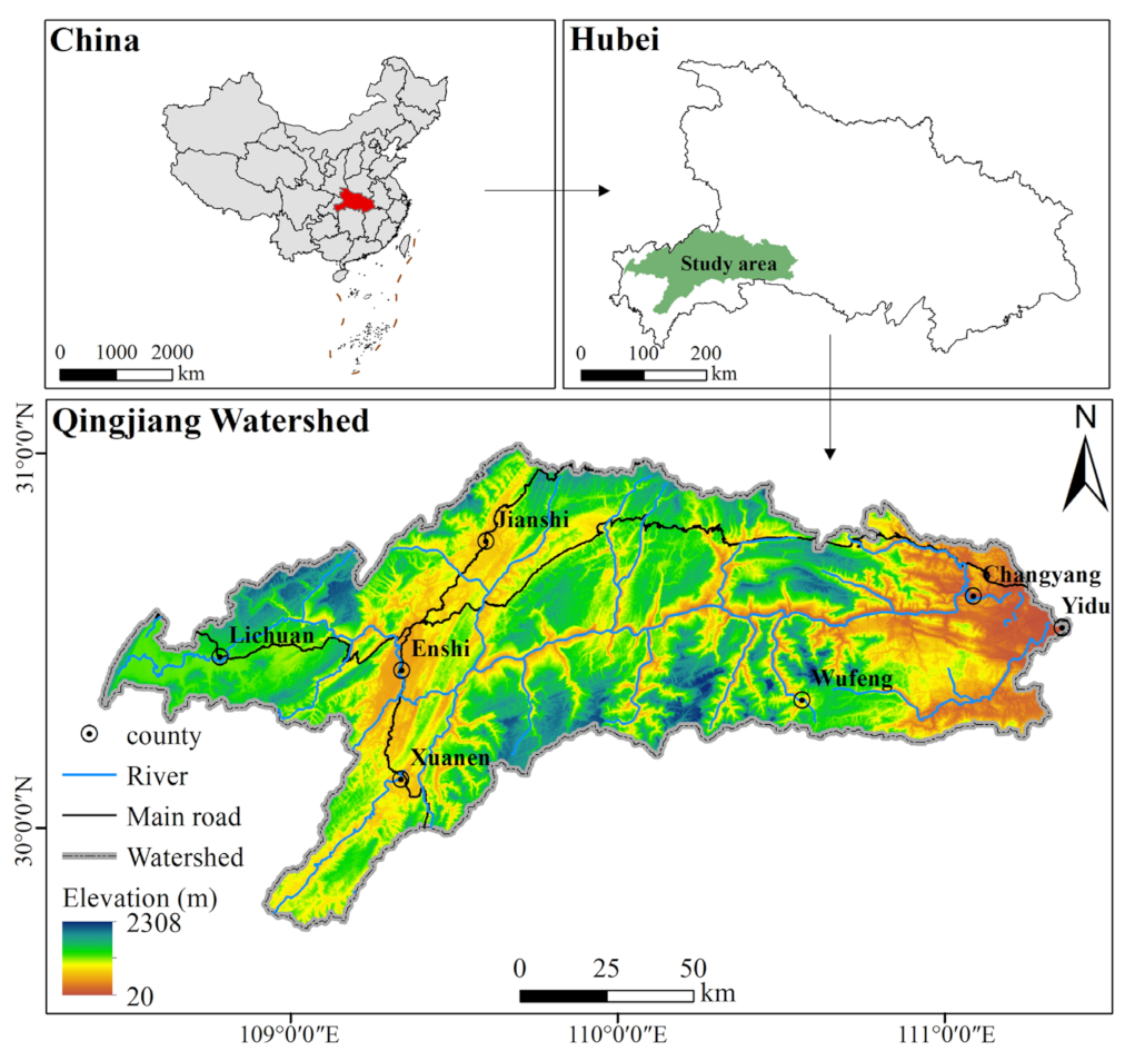
2.1. Study Area

The Qingjiang Watershed in southwestern Hubei (29°33′–30°50′N, 108°35′–111°35′E) is a typical mountainous basin, with a total area of 16,800 km² (Figure 1). The climate of the QJW is subtropical monsoon, with annual precipitation of 1420 mm and annual average sunshine hours ranging from 1160–1600 h. Except for some basins and alluvial plains, the primary geomorphic type of the QJW is mountain, with an area proportion of 80%. The Qingjiang River flows from west to east through Lichuan, Enshi, Xianfeng, Xuanen, Jiansi, Badong and Hefeng in Enshi Tujia and Miao Autonomous Prefecture, and Changyang, Wufeng and Yidu in Yichang City. Except for Yidu City, the rest of the QJW belongs to the Wuling Mountains, known for economic backwardness and an aging population. Containing several national nature reserves, the QJW has nationally critical ecological functions of soil and water conservation and biodiversity maintenance. Meanwhile, the hydraulic engineering of the QJW has enabled the watershed to assume water storage, power generation and flood control functions.

2.2. Data Sources

This study used multiple data sources to calculate four ESs in the QJW and explore the impacts of land use change on ESs based on land use simulation, including land use maps, meteorological data, soil, topography, vegetation, socio-economic and basic geographic data. By calculating the daily meteorological data of 27 weather monitoring stations, we obtained the annual average precipitation and temperature in 1990, 2000, 2010 and 2018, and we used the inverse distance interpolation method to convert the above data to raster format. The spatial resolution of all raster images was resampled into 30 m in this study. All data coordinates were unified into a Gauss–Krüger projection. More information about the multiple data is shown in

Table 1. The details of data used in this study.

Data Name	Description	Resolution	Format	Data Source
Land use data	Land use maps generated from satellite images in 1990, 2000, 2010 and 2018	30 m	Raster	The Resource and Environment Science and Data Center of the Chinese Academy of Sciences: https://www.resdc.cn/ (accessed on 20 June 2020)
Meteorological data	27 stations around the QJW providing daily precipitation and average, maximum and minimum temperatures in 1990, 2000, 2010 and 2018	-	Shapefile	The China Meteorological Science Data Sharing Service website: http://data.cma.gov.cn/ (accessed on 1 July 2020)
Soil	Including soil depth, organic content, and percentages of sand, clay and powder particles	1 km	Raster	The Harmonized World Soil Database (v1.1) from the National Glacial Permafrost Desert Scientific Data Center: http://www.ncdc.ac.cn/ (accessed on 20 June 2020)
Topography	Digital elevation model	30 m	Raster	The Geospatial Data Cloud: http://www.gscloud.cn/ (accessed on 5 September 2020)
Vegetation	Annual maximum of normalized difference vegetation index (NDVI) and leaf area index (LAI) in 1990, 2000, 2010 and 2018	1 km	Raster	The Resource and Environment Science and Data Center of the Chinese Academy of Sciences: https://www.resdc.cn/ (accessed on 20 September 2020)
Socio-economic data	Including gross domestic product (GDP) and population density (POP) in 1990, 2000, 2010 and 2019	1 km	Raster	The Resource and Environment Science and Data Center of the Chinese Academy of Sciences: https://www.resdc.cn/ (accessed on 15 March 2021)
Basic geographic data	Including the administrative zones, railroads, main roads and watersheds	-	Shapefile	The Resource and Environment Science and Data Center of the Chinese Academy of Sciences: https://www.resdc.cn/ (accessed on 1 March 2021)

.

2.3. Ecosystem Services Assessment

Considering the geographical conditions and ecological sensitivity of the QJW, we calculated four ESs: water yield, soil conservation, carbon sequestration and habitat quality. The following parts introduce these four modules of the InVEST.

2.3.1. Water Yield (WY)

WY represents the availability of water resources in a watershed, influenced by factors such as land use pattern, climate, topography and soil characteristics [25,26]. The WY module calculates the discrepancy between precipitation and actual evapotranspiration at the scale of a watershed. The model can be expressed as follows:

$$Y_i=\left(1-\frac{AE{T}_i}{P_i}\right)\cdot P_i$$

(1)

$$\frac{AE{T}_i}{P_i}=1+\frac{PE{T}_i}{P_i}-{\left[1+{\left(\frac{PETi}{P_i}\right)}^{\omega }\right]}^{\frac{1}{\omega }}$$

(2)

$$PE{T}_i=K_c\left(l_i\right)\cdot E{T}_{0i}$$

(3)

$${\omega }_i=Z\frac{AW{C}_i}{P_i}+1.25$$

(4)

where $Y_i$ is the annual WY (mm); $P_i$ is the annual precipitation (mm); $AE{T}_i$ is the annual evapotranspiration (mm); $PE{T}_i$ is the potential evapotranspiration; $E{T}_{0i}$ is the vegetation evapotranspiration; $K_c\left(l_i\right)$ is the crop evapotranspiration coefficient; $AW{C}_i$ is the water content available to plants; ${\omega }_i$ is the empirical parameter; and $Z$ is the Zhang parameter which characterizes the hydrogeological features of a given region.

The input data included land use/cover, precipitation, potential evapotranspiration ($E{T}_0$), plant available water content (PAWC), soil and root depth, $Z$ score, and crop evapotranspiration coefficient ($K_c$). The $E{T}_{0i}$ was estimated using the ‘Modified Hargreaves’ equation [27], which is as follows:

$$E{T}_0=0.0013\times 0.408\times RA\times \left(T_{av}+17\right)\times {(TD-0.0123P)}^{0.76}$$

(5)

where $E{T}_0$ is the potential evapotranspiration (mm); $RA$ is the solar atmospheric topside radiation (MJ·m⁻²·d⁻¹); $T_{av}$ is the average of the mean daily maximum and minimum temperatures (°C); $TD$ is the average of the mean daily maximum and minimum temperatures (°C); and $P$ is the average monthly precipitation (mm).

PAWC was calculated using the formula of vegetation available water [28], which is as follows:

$$\begin{array}{c}PAWC=54.509-0.132\times SAN-0.003\times {(SAN)}^2-0.055\times {(SIL)}^2\\ -0.738\times CLA+0.007\times {(CLA)}^2-2.688\times OC+0.501\times {(OC)}^2\end{array}$$

(6)

where $SAN$ is the soil sand grain (%); $SIL$ is the soil powder grain (%); $CLA$ is the soil clay grain (%); and $OC$ is the soil organic carbon content (%), which was obtained by dividing organic matter by 1.724 in this study.

The soil depth was obtained from the Harmonized World Soil Database, and the root depth came from the InVEST user’s guide [29] (Supplementary Materials Table S1). The value of Z was revised based on the related research, which was taken as 3 [30]. The $K_c$ was calculated using the empirical formula based on the relationships between $K_c$ and $LAI$ [31], which is as follows:

$$K_c=\left\{\begin{array}{l} \frac{LAI}{3}, LAI\le 3\\ 1\end{array}\right.$$

(7)

where $K_c$ is the vegetation evapotranspiration coefficient and $LAI$ is the leaf area index.

2.3.2. Soil Conservation (SC)

SC reflects the capacity of different land use types to resist soil erosion and their ability to retain soil under varying conditions [26,32]. The SDR module calculates the total soil conservation through the summation of soil erosion reduction and retention [33]. The model can be expressed as follows:

$$RKL{S}_i=R_i\cdot K_i\cdot L{S}_i$$

(8)

$$USL{E}_i=R_i\cdot K_i\cdot L{S}_i\cdot C_i\cdot P_i$$

(9)

$$L{S}_i=S_i\frac{{\left(A_{i-in}+D^2\right)}^{m+1}-A_{i-in}^{m+1}}{D^{m+2}\cdot x_i^m\cdot {(22.13)}^m}$$

(10)

$$SEDRE{T}_i=RKL{S}_i-USL{E}_i+se{d}_{expor{t}_i}$$

(11)

where $RKL{S}_i$ is the potential soil erosion (t·ha⁻¹·yr⁻¹); $USL{E}_i$ is the actual soil erosion (t·ha⁻¹·yr⁻¹); $R_i$ is the rainfall erosion (MJ·mm(ha·hr·yr)⁻¹); $K_i$ is the soil erosion factor (t·ha·hr(MJ·ha·mm)⁻¹); $L{S}_i$ is the slope length–gradient coefficient; $S_i$ is the slope factor calculated as a function of slope; $A_{i-in}$ is the contributing area at the inlet of a grid cell i which is computed from the Multiple-Flow Direction method (m²); $D$ is the grid cell linear dimension ($m$); $x_i$ is the mean of an aspect weighted by proportional outflow; $C_i$ is the crop management coefficient; $P_i$ is the practice coefficient; $SEDRE{T}_i$ represents the soil retention; $RKL{S}_i-USL{E}_i$ represents the retention of sediments; and $se{d}_{expor{t}_i}$ represents the amount of sediment intercepted upstream.

The input data for the SC module included DEM, land cover, rainfall erosion index ($R$), soil erosion index ($K$), crop management factor ($C$) and support practice factor ($P$). The R factor was calculated using the monthly scale formula [34], which is as follows:

$$R=\underset{1}{\sum ^{12}}\left(1.735\times {10}^{\left(1.5lg\left(\frac{P_i^2}{P}\right)-0.8188\right)}\right)$$

(12)

where $R$ is the rainfall erosion (MJ·mm(ha·hr·yr)⁻¹); $P_i$ is the monthly precipitation (mm); and $P$ is the annual precipitation (mm). The unit of $R$ in this formula is 100 ft·sht·in/(ac·h·y), which needs to be converted to the international unit MJ·mm(ha·hr·yr)⁻¹ by multiplying it by 17.02.

The K factor was calculated using the revised EPIC formula [35], which is as follows:

$$\begin{array}{c}{K}_{EPIC}=\left\{0.2+0.3exp\left[-0.0256SAN\left(1-SIL/100\right)\right]\right\}{\left[\frac{SIL}{CLA+SIL}\right]}^{0.3}\\ \left[1.0-\frac{0.25\mathrm{O}C}{OC+exp\left(3.72-2.95\mathrm{O}C\right)}\right]\left[1.0-\frac{0.7SN}{SN+exp\left(-5.51+22.9SN\right)}\right]\end{array}$$

(13)

$$K=\left(-0.01383+0.51575K_{\mathrm{EPIC} }\right)\times 0.1317$$

(14)

where $K$ is the soil erodibility factor (t·ha·hr(MJ·ha·mm)⁻¹); $SAN$ is the soil sand grain (%); $SIL$ is the soil powder grain (%); $CLA$ is the soil clay grain (%); $SN$ = 1 − $SAN/100$; and $OC$ is the soil organic carbon content (%). The $C$ and $P$ in this study were estimated based on the related studies [32,36,37] (Table S2).

2.3.3. Carbon Storage (CS)

CS is crucial for regional climate regulation [38]. The Carbon Storage and Sequestration model of InVEST quantifies the total carbon stored in a landscape or the amount of carbon sequestered over time [39]. The model can be expressed as follows:

$$C_i=C_{\mathrm{a}}+C_{\mathrm{b}}+C_{\mathrm{c}}+C_{\mathrm{d}}$$

(15)

where $C_i$ is the carbon density of ecosystem type i (t·ha⁻¹); $C_{\mathrm{a}}$ is the aboveground carbon density (t·ha⁻¹); $C_{\mathrm{b}}$ is the underground carbon density (t·ha⁻¹); $C_{\mathrm{c}}$ is the density of dead organic carbon (t·ha⁻¹); and $C_{\mathrm{d}}$ is the soil carbon density (t·ha⁻¹).

The input data for the CS module mainly included land cover and carbon pools (Table S3), which had four types of carbon density values above based on those derived from related studies [29,40,41].

2.3.4. Habitat Quality (HQ)

HQ is used to assess the capacity of an ecosystem to sustain the ongoing viability and propagation of species [42]. The HQ module of InVEST combines land use and other threat source factors. The model can be expressed as follows:

$$Q_{xj}=H_j\left(1-\left(\frac{D_{xj}^z}{D_{xj}^z+k^z}\right)\right)$$

(16)

where $Q_{xj}$ is the habitat quality of pixel x within land use type j; $H_j$ is the habitat suitability of land use type j; $D_{xj}^z$ is the habitat degradation within land use type j; k is the half-saturation coefficient; and Z is the normalization constant. Meanwhile:

$$D_{xj}=\underset{r=1}{\sum ^R}\underset{y=1}{\sum ^{Y_r}}\left(\frac{w_r}{{\sum }_{r=1}^R{w}_r}\right)r_y{i}_{rxy}{\beta }_x{S}_{jr}$$

(17)

where $R$ is the number of stress factors; $y$ is the total pixel number of stress factor r; $Y_r$ is the number of pixels occupied by stress factor r; $w_r$ is the weight-assigned stress factor r; $r_y$ is the stress factor value of pixel y; $i_{rxy}$ is the degree of stress of pixel x by the stress factor value of $r_y$; ${\beta }_x$ is the level of accessibility for a stress factor; and $S_{jr}$ is the sensitivity of land use type j to stress factor r. The model provides two distance decay functions for calculating the variation of stressors with distance: linear decay and exponential decay.

The input data for the HQ module included land cover, stress factors and their maximum influence on distance and weight, habitat suitability and sensitivity to different stress factors. We chose seven stress factors according to the characteristics of the QJW (Table S4). The parameters for the maximum influence distance and weight of stress factors, as well as the habitat adaptability and sensitivity values of the various land use types, were obtained from the relevant literature in similar geographic regions [43,44] (Tables S4 and S5).

2.4. Simulating Land use Patterns Based on the Logistic–CA–Markov Model

2.4.1. Logistic–CA–Markov Model

The Logistic–CA–Markov model has been used to simulate regional land use/cover patterns in different regions [45,46,47], combining logistic regression, which selects variables that significantly influence land use patterns of the QJW, and the CA–Markov model, which integrates Cellular Automata (CA) and the Markov model to predict the spatial and temporal dynamics of land use structure. In this study, we used this model in IDRISI Selva software to predict four kinds of land use patterns of the QJW in 2034.

Logistic regression is a categorical analysis of multiple variables, which can be expressed as follows:

$$logistic\left(\frac{P_i}{1-P_i}\right)={\beta }_0+{\beta }_1{X}_1+{\beta }_2{X}_2+\cdots +{\beta }_n{X}_n$$

(18)

where $P_i$ is the probability that a particular land use type i may occur in each grid; ${\beta }_0$ is a constant; ${\beta }_{\mathrm{j}}\left(j=1,2,\dots ,n\right)$ is the coefficient of each driver of the regression equation; and $X_{\mathrm{j}}\left(j=1,2,\dots ,n\right)$ is each input driver.

The CA model is a dynamical system discrete in both time and space [48], which is defined by constitutive rules. The model consists of five components: metacell, metacell space, state, domain and rules, which can be expressed as follows:

$$S_{t+1}^{\prime }=\left(U_d,S_t^{\prime },N_t,f\right)$$

(19)

where $S_{t+1}^{\prime }$ is the metacell state at moment t+1; $U_d$ is the d-dimensional metacell space; $S_t^{\prime }$ is the metacell state at moment t; $N_t$ is the combination of neighborhood states at moment t; and 𝑓 is the transition rule of the local space metacell.

The Markov model uses the present state of a system and its development trend to predict the future trend, which is a stochastic type of time series prediction model based on probability. The state of the process at the moment t+1 is only relevant to the moment t, which can be expressed as follows:

$$P=P_{ij}\left(n\right)=\left[\begin{array}{ccc}{P}_{11}& \cdots & P_{1n}\\ ⋮& \ddots & ⋮\\ P_{n1}& \cdots & P_{nn}\end{array}\right]$$

(20)

$$S_{t+1}=S_t\cdot P$$

(21)

where $S_{t+1}$ is the state probability of the land use system at moment t+1; $S_t$ is the state probability at moment t; $P$ is the state transfer matrix; and $P_{ij}$ is the land type i transformed into j.

2.4.2. Simulating Process Design

To simulate the land use scenario in 2034, we first used the Markov model to calculate the area matrix of the land use/cover transfer from 2010 to 2018, with the background raster cell assigned to 0 and the scale error set to 0.15.

Second, the logistic regression model was used to calculate the occurrence probability of each land type on each raster cell separately. In this study, the changing area of cropland, forest land, grassland, water, construction land and unused land were used as dependent variables. Based on three aspects (natural environment, socio-economic conditions and geographical location), the following 11 representative indicators were finally determined as drivers: elevation, slope, aspect, precipitation, temperature, population density, GDP, distance to towns, distance to rural residential areas, distance to rivers and distance to major roads [20].

Third, the CA–Markov model was used to predict the future land use/cover pattern. The metacell space of this study was the Qingjiang Watershed, the metacell state was six land use types and the metacell size was the raster size 30 × 30 m. The land use distribution map in 2018, the Markov transfer matrix area under different development scenarios from 2010 to 2018 and the suitability probability distribution of 2018 were entered into the CA–Markov model. The metacell neighborhood was a 5 × 5 filter and the number of iterations was set to 16.

2.4.3. Model Validation

To verify the feasibility of the land use simulation process, we used the ROC test and the validate module in IDRISI Selva software. The ROC test can determine whether the predicted distribution is the highest suitable area. If the value is higher than 0.7, the model fits the data well. The validation module can detect the consistency of various classification quantities and locations of the two images, and generate standard kappa (Kstandard), random kappa (Kno), locational kappa (Klocation) and stratified location kappa (KlocationStrata) coefficients. If the coefficient is higher than 0.75, the consistency of the two comparison images is excellent and the prediction is accurate. If the value is close to 1, the simulation result is more accurate. We first simulated the land use patterns for 2010 and 2020. As we lacked the land use data in 2020, we used the data from 2018 for validation instead. The results of the ROC test and the validation module of 2010 and 2020 are shown in Tables S6 and S7, which indicated that this simulation process is feasible.

2.4.4. Scenario Setting

As a national ecological area of soil and water conservation and biodiversity, the QJW is situated in the mountainous region of southwestern Hubei Province, where Badong and Yidu counties are promoted for developing ecological tourism in the watershed. There are many relevant planning projects and policies regarding the QJW, such as “the Hubei Yangtze River Economic Belt Ecological Environmental Protection Plan (2016–2020)”, “the Regulations on Water and Ecological Environmental Protection in the Qingjiang River Basin of Hubei Province”, “the Comprehensive Utilization Plan in the Qingjiang Basin of Enshi Prefecture (2011–2020)” and “Implementing large-scale protection and avoiding large-scale development of the Yangtze River Basin”. To assess the effect of LUCC on ESs, we designed four hypothetical land use scenarios of the QJW for the year 2034, considering the location and resource features of this area (

Table 2. The description of four land use scenarios designed in this study.

Scenario Type	Description	Parameter Setting
Business as Usual (BAU)	To maintain the natural development trends from 2010 to 2018	The demand for land use types was calculated from the land use data in 2018 and the conversion likelihood of land use during the 2010–2018 period.
Ecological Land Protection (ELP)	To promote the priority development of an ecological environment	Hotspot analysis can provide a more comprehensive assessment of ES supply and aims to improve the management level of ESs in a watershed [49]. One ecosystem service’s hotspot is where the service value exceeds its mean value that year. The four ES hotspots are where the four kinds of ESs exceed their mean value, representing the high value of ecological protection. Converting the four ES hotspots to built-up land was prohibited. The conversion likelihood of forest, grassland and water to built-up land was reduced by 100%, and the likelihood of conversion to cropland was reduced by 100%, 50% and 10%, respectively. The conversion likelihood of cropland to forest land, grassland and water was augmented by 30%, and the conversion likelihood to construction land was decreased by 10%.
Arable Land Protection (ALP)	To consider the security and production of food to meet the food needs of an increasing population	The cropland in the mountainous area requires better natural conditions, highlighting the significance of the red-line policy of arable land. The conversion likelihood of cropland to forest land, grassland and water was reduced by 30%, and the conversion likelihood to built-up land and unused land was decreased by 100%. The conversion likelihood of other land use types to cropland was augmented by 30%.
Ecological Economic Construction (EEC)	To create more sustainable and human-centered growth strategies based on ecological protection with rational utilization of natural resources and practical economic construction under regional conditions	Converting the four ES hotspots to built-up land was prohibited. The conversion likelihood of cropland and unused land to forest land, grassland and water was increased by 10%, and the conversion likelihood of grassland to forest land was increased by 10%. The conversion likelihood of other land use types to built-up land was increased by 10%. The conversion likelihood of built-up land to arable land and unused land was decreased by 100%, and the conversion likelihood to woodland, grassland and water was reduced by 30%.

).

2.5. Exploring Possible Factors Affecting ESs in the QJW

2.5.1. Geographical Detector

The geodetector, which includes four different detector types, is an advanced tool used to identify the spatial heterogeneity characteristics of variables [50,51]. The q-statistic is used to quantify the effect of different factors on the spatial heterogeneity of ESs, which is written as:

$$q=1-\frac{{\sum }_{h=1}^l{N}_h{\sigma }_h^2}{N{\sigma }^2}$$

(22)

where q is the explanatory influence of factor X on Y; N is the number of geographical units; $N_h$ is the number of units in the subdivision h; l is the total number of subdivision units; and ${\sigma }^2$ and ${\sigma }_h^2$ are the variance of Y in a whole area and in each subdivision, respectively. A higher value of q means a more substantial effect of X on Y.

We used the factor detector to explore the effect of different variables on the spatial heterogeneity of ESs and the interaction detector to assess the interactive impacts of variables on ESs in the QJW from 1990 to 2018. Considering the topography, climate, vegetation and socio-economic conditions of the QJW, the independent variables in this study were elevation, slope, terrain, precipitation, temperature, NDVI, land use type, GDP and POP. The dependent variables were WY, SC, CS and HQ. The elevation was extracted from the DEM and the slope was calculated by entering the DEM data into the slope calculation tool of ArcGIS 10.7. Considering the geographic conditions of QJW, the watershed terrain was divided into five categories: plain (undulation 0–20 m), hill (elevation < 500 m; elevation > 500 m, undulation 20–150 m), low mountain (elevation 500–800 m, undulation > 150 m), intermediate mountain (elevation 800–2000 m, undulation > 20 m) and high mountain (elevation 2000–3000 m, undulation > 20 m) [52]. The undulation in this study was calculated using the focus statistics tool of ArcGIS 10.7. The research area was partitioned into intervals of 2 km, resulting in the generation of 4197 sampling points to collect variables. The study utilized the equivalence and natural break methods to divide the data into intervals with a range of 5 to 7. Moreover, we conducted the variation inflation factor (VIF) to check the redundancy of the input variable. If the VIF value of one factor is less than 7.5, the factor is recommended for calculation [53]. The VIF diagnostic results of chosen independent variables from 1990 to 2018 are shown in Table S8.

2.5.2. Multiscale Geographically Weighted Regression (MGWR)

MGWR explores the effects of the spatial characteristics of different independent variables on the dependent variable by using a back-fitting algorithm to exploit the optimal bandwidth of each variable and calibrate model fitting accuracy [54]. Compared to GWR, this method can estimate parameters of input factors at different spatial scales and reduce covariance interference, which is written as:

$$y_i=\underset{j=0}{\sum ^m}{\beta }_{bwj}\left(u_i,v_i\right)x_{ij}+{\epsilon }_i$$

(23)

where $y_i$ is the dependent variable; $x_{ij}$ is the jth coefficient; $bwj$ in ${\beta }_{bwj}$ is the bandwidth used for calibration of the jth conditional relationship; and ${\epsilon }_i$ is the error term.

In this study, we used MGWR to investigate the spatial influence of each major land use type on the distribution of each ES heterogeneity in the QJW. To improve the fitting effect of MGWR modeling, we ranked the explanatory power of all factors’ outputs using the factor detector in Section 2.5.1 from highest to lowest, and the top five factors were selected for further MGWR modeling. If the top five factors of each ES did not contain land use type data, the type data were additionally added to the modeling analysis. Considering the representativeness and reliability of the calculation results, this paper chose to take the results of 2018 as an example for MGWR calculation. The main factors of each ES used in MGWR modeling are shown in Table S9. If two values were very close to each other and only one could be selected, the category of the factor was considered and the one that was different from the selected factor was selected based on the principle of diversity.

3. Results

3.1. Characteristics of Land Use/Cover Change in the QJW from 1990 to 2018

3.1.1. Temporal Analysis of Land Use/Cover Change in the QJW

The land use/cover of the QJW in the past 40 years was dominated by woodland, accounting for about 80% of the basin area (Figure 2b). This was followed by cropland and grassland, accounting for about 12% and 8%, respectively. The area proportion of water bodies and construction land was deficient, within 1%. From 1990 to 2018, the most significant LUCC in the watershed was a reduction in the forest land area, totaling 138.17 km² (Figure 2c). This was followed by increases in construction land and water of 96.65 km² and 88.78 km², respectively. The cropland, grassland and unused land decreased by 28.3 km², 18.76 km² and 0.21 km², respectively. In the QJW, the LUCC was insignificant before 2000, and more changes occurred after 2000. These were mainly concentrated during the 2000–2010 period, with an increase of 88.39 km² and 57.63 km² in water and construction land, respectively, and a decrease of 83.94 km², 32.66 km² and 29.62 km² in the woodland, cropland and grassland, respectively. The area of each type maintained the same trend of change from 2010 to 2018, with different levels of decrease.

Forest land was the primary type of land converted to cropland, grassland, water bodies and built-up land, with areas of 481.40 km², 132.96 km², 95.18 km² and 62.10 km², respectively (Figure 3). Cropland, grassland, water and built-up land were mainly converted to forest land, with areas of 464.00 km², 148.84 km², 17.09 km² and 3.50 km², respectively. The area of cropland and grassland converted to forest land was close to the area of forest land converted to cropland and grassland. The area of water bodies and built-up land converted to woodland was much smaller than the area of forest land converted to water bodies and built-up land.

3.1.2. Spatial Distribution of Land Use/Cover Change in the QJW

The spatial pattern of land use transfers had apparent heterogeneity in the QJW during 1990–2018 (Figure 4). The mutual transfer of cropland and forest land was distributed in various places within the watershed. The forest land converted to cropland was distributed along the river in the Saidu and Zhiluo river basins (Figure 4a). The cropland converted to forest land was distributed more in the Tianchi and Saidu rivers (Figure 4b). After 2000, the most significant amount of land converted to water bodies was forest, which was concentrated on both sides of the Qingjiang River, especially in the middle and lower reaches. Three projects of the middle and lower reaches of the Qingjiang River are Gao Bazhou, Geheyan and Shuibuya (in order of water storage level from low to high), with Shuibuya hydropower station as the leader of the Qingjiang River terrace development. After the opening of the Shuibuya station in 2002, the water volume in the middle reaches increased significantly (Figure 4d). Due to the increase in water storage at the Shuibuya station, the water volume in the watershed between it and the Geheyan station decreased, increasing the area of forest land (Figure 4c). Forest land was the primary type of land converted to construction land, concentrated in the center of Enshi City and on both sides of some significant transportation roads, such as the Shanghai–Chongqing high-speed railway (G50) and the Enshi–Qianjiang Expressway (S89) (Figure 4e).

3.2. Spatiotemporal Analysis of ES Change in the QJW from 1990 to 2018

3.2.1. Temporal Analysis of ES Change in the QJW

During 1990–2018, the values of WY showed an uptrend, increasing from 669.40 to 796.07 mm. Meanwhile, the SC, CS and HQ showed a downtrend, decreasing by 44.80 t·ha⁻¹, 0.12 t·ha⁻¹ and 0.003, respectively (Figure 5a). The average WY was 802.67 mm between 1990 and 2018, and the WY increased significantly before 2000 and maintained a decreasing trend after 2000, with the maximum in 2000 and the minimum in 1990. The average of SC was 137.08 t·ha⁻¹, and the change rate of SC slowed down after 2000, with a significant decline from 1990 to 2000. The average of CS and HQ was 11.56 t·ha⁻¹ and 0.74, respectively. The CS and HQ reduced weakly, with the maximum in 1990 and the minimum in 2018.

In this paper, the Z-Score method and the radar plot were used to standardize ES values and visualize the relationships of ESs in different years, respectively (Figure 5b). During 1990–2018, the relationships of the three ESs (HQ > CS > SC) remained stable. The dominant ES was HQ from 1990 to 2000, replaced by WY from 2000 to 2018, and the value of SC was the lowest among the four ESs.

3.2.2. Spatial Distribution of ES Change in the QJW

The WY values were high in the southwestern QJW and decreased from the southwest to the northeast during the 1990–2018 period (Figure 6). The high values of SC were primarily distributed in the valleys, which were located along the main river and tributaries of the midstream and downstream, and the low values were distributed in the large basins in Lichuan, Jianshi and Enshi counties and the plains of the eastern estuary. Compared to the upstream area, the water volume increased in the midstream and downstream areas, where the terrain of the river sides was relatively flat and the river widened, which made the SC value larger. The highest values of CS were located in the woodland of the QJW. The lowest values of CS were concentrated in the upstream and downstream estuary and the northern QJW, the land types of which were mainly built-up land, water and grassland. The lowest values of HQ were primarily distributed in the built-up areas of the QJW, such as Enshi, Yidu and Lichuan counties, the landforms of which were mostly plains or basins, where disturbances from human activities are more likely to exist.

3.2.3. Analysis of ES Change in Main Land Use Types in the QJW

The summed areas of arable land (AL), forest land (FL) and grassland (GL) account for about 90% of the QJW, so this paper focused on the ES changes in these land use types (Figure 7). Among these three land use types, AL had the largest WY, with values between 800 and 1100 mm, followed by GL. WY in AL and GL was greater than the average of the QJW, and WY in FL was lower than the QJW. During 1990–2018, the value trend of the three types remained consistent with the watershed, with WY rising before 2000 and falling and then rising again after 2000. The ranking of SC in three land use types was: FL > AL > GL, where only the SC in FL was greater than the watershed. The SC in FL declined from 180 to 130 t·ha⁻¹ from 1990 to 2018, maintaining a fluctuating decline. The CS in FL was the highest among the three types, with a value around 13 t·ha⁻¹ higher than the QJW. The HQ in FL was greater than 0.8, exceeding the HQ of the QJW, and the HQ in AL was the smallest, with a value of around 0.3. The values of CS and HQ remained stable among the three main land use types between 1990 and 2018.

Figure 8 showed the effect of arable land and forest land area on the spatial heterogeneity of the four ESs in the QJW in 2018. The increase in cropland area had a negative effect on WY in a few areas, such as the basin centered on Lichuan and Jianshi counties, and a positive effect on WY in most areas, with high values mainly in the eastern part of the basin centered on Wufeng and Changyang counties. The area of positive effect of forest area on WY was similar to that of cropland, which was mainly distributed in the eastern and southwestern part of the basin. As the main provider of SC in the QJW, the role of woodland shifted from positive to negative from west to east, with the positive role mainly concentrated in the western part of the QJW. The increase in the woodland area had a positive effect on both CS and HQ in the whole watershed, and the overall trend showed a gradual increase from west to east.

3.3. Multi-Scenario Prediction of ESs in the QJW in 2034

3.3.1. Characteristics of Land Use/Cover Change in the QJW in 2034

The predicted land use structure in 2034 was still dominated by forest land, the area of which under each scenario was ranked as follows: ELP (14,651.12 km²) > EEC (11,773.66 km²) > BAU (11,699.23 km²) > ALP (11,309.25 km²). Under the ELP, the area proportion of cropland was 86.96% (Figure 9a). Under the remaining three scenarios, the proportion of forest area decreased to about 70%. The cropland area in each scenario was ranked as ALP (3562.97 km²) > BAU (3090.28 km²) > EEC (2990.89 km²) > ELP (937.34 km²). Compared to the year 2018, all scenarios increased the cropland area by more than 1000 km² and decreased the forest area by more than 1400 km², except for the ELP scenario, which reduced the area of cropland by 1008.78 km² and increased the area of forest land by 1384.05 km² (Figure 9b). The areas of grassland and water were the largest under the BAU, at 1525.74 km² and 243.52 km², respectively, and were the smallest under the ELP, at 181.73 km² and 102.53 km², respectively. The area of built-up land was ranked as follows: EEC (338.65 km²) > BAU (288.84 km²) > ALP (234.61 km²) > ELP (102.56 km²). The built-up land under the EEC increased by 206.19 km² and under the ELP decreased by 29.9 km².

The land use pattern of the QJW under four policy scenarios had apparent land use conflicts, mainly in arable land and construction land (Figure 10). Compared to the land use in 2018, under BAU, cropland growth was mainly distributed in the northwestern Lizhong Basin, the southwestern low mountains and the basins in the central areas of Enshi City, with a northeast–southwest orientation. Meanwhile, the arable land growth was distributed downstream of the Qingjiang River estuary and the Yuyang River basin. The development of built-up land was concentrated in the center of Enshi City, with a slight increase in Yidu City and Changyang County. Under ELP, most of the fragmented arable land was transferred to forest land. The arable land was mainly distributed in the northwestern watershed and near the estuary in the east, where the land was relatively fertile and the topography was less undulating, with better conditions for agricultural cultivation. The increase in arable land under the ALP was similar to that under the BAU, showing contiguous growth. The distribution of built-up land under the EEC was similar to that under the BAU, with the most significant increase in Enshi City.

3.3.2. Spatiotemporal Pattern of ESs in the QJW in 2034

The WY reduced to a range of 700–721 mm compared with the values in 2018, with the values ranked as follows: ALP (−75.35 mm) > BAU (−77.94 mm) > EEC (−78.49 mm) > ELP (−93.51 mm) (Figure 11a). The SC increased to around 135 t·ha⁻¹ under the four scenarios, with the SC values ranked as follows: ALP (+14.14 t·ha⁻¹) > BAU (+13.91 t·ha⁻¹) > EEC (+13.81 t·ha⁻¹) > ELP (+13.69 t·ha⁻¹), which was the same rank as WY. The CS increased to the range of 13.66–16.65 t·ha⁻¹, with the ranking as follows: ELP (+5.15 t·ha⁻¹) > EEC (+2.56 t·ha⁻¹) > BAU (+2.5 t·ha⁻¹) > ALP (+2.16 t·ha⁻¹), which was the opposite of WY and SC. The HQ ranged from 0.80 to 0.93, and the values were ranked as follows: ELP (+0.197) > EEC (+0.087) > BAU (+0.087) > ALP (+0.067).

SC dominated the structure of ESs in the QJW in 2034, and the main difference in ES structure under the four scenarios was the change of HQ (Figure 11b). The BAU and ELP scenarios had the same structure of ES: SC > HQ > WY > CS, while the ALP and EEC scenarios had the same structure: SC > WY > CS > HQ.

The spatial pattern of WY and SC remained the same in 2034, while the spatial heterogeneity of CS and HQ reduced compared with the period from 1990 to 2018 (Figure 12). In general, the WY distribution still decreased from southwest to northeast in the QJW. The distribution of WY under the BAU and ELP scenarios was similar, while the distribution under the ALP and EEC scenarios was also similar. Under the four land use scenarios, the spatial distribution of SC was almost the same. Except for the ELP, the spatial pattern of CS was similar under the BAU, ALP and EEC scenarios, with high values in the middle and lower reaches and low values in the upper reach. The growth of HQ was primarily located in the forest land of QJW, with the most significant increase under the ELP.

3.3.3. ESs in Main Land Use Types in the QJW in 2034

The WY in AL maintained the highest value among the three land use types (Figure 13). The ranking of WY in AL under the four simulation scenarios was EEC > BAU > ALP > ELP, and the values of the first three scenarios were relatively closer. The WY in AL under the ELP scenario was the lowest, with a value of 804.02 mm. The ranking of WY in FL was ELP > EEC > BAU > ALP, and the WY in FL under the ELP was 696.50 mm lower than the WY of the watershed. The SC in FL sustained the highest value among the three land use types, and the ranking among the four scenarios was ALP > EEC > BAU > ELP. Except for in the ELP scenario, the other three were greater than 150 t·ha⁻¹. The ranking of CS and HQ in the three main land use types under the four scenarios was FL > GL > AL. Compared to the period from 1990 to 2018, the CS in FL increased to about 18 t·ha⁻¹, and the CS in AL decreased to less than 4 t·ha⁻¹. The HQ in FL in 2034 increased to a near-value of 1, while the HQ in GL decreased to below 0.6.

4. Discussion

4.1. Application of MGWR Model in Exploring Spatial Heterogeneity of Ecosystem Services

MGWR is a relatively new spatial analysis statistical method that has been used in many fields such as air pollution monitoring [55,56], disease and health surveillance [57,58], and traffic accident prediction [59]. Compared with GWR and OLS models, this method adopts an adaptive bandwidth method and introduces a local spatial weight matrix to consider the spatial correlation between sample points, which can effectively solve the spatial non-stationarity problem of the research object. It also identifies local changes in variable relationships to generate localized parameters and produces finer prediction results. In addition, since the MGWR model can adjust the spatial weight, it can reduce the influence of outliers, increasing the stability and reliability of the prediction results [54]. The prediction verification results of the OLS and MGWR models shown in Table S10 indicate that the results of the MGWR model have significantly higher R² and smaller AICc values, with stronger data interpretation and prediction accuracy.

The MGWR model can reduce the spatial scale effects of different factors on the research subjects and clarify the specific scope of different variables, which can more precisely determine the influence of major driving factors on different ecosystem services [60]. Before using the MGWR model in this study, the geographical detector model was first used to screen the dominant driving factors of different ESs to reduce the collinearity interference between the input factors and improve the prediction efficiency and accuracy of the MGWR model. Since this paper focuses on the mechanism of land use changes on ESs, the bandwidth size and local regression coefficients of different factors were calculated to quantify the influence of the main land use type variables in the QJW on the spatial heterogeneity of ESs. Taking the forest area factor as an example, the larger the bandwidth of the forest area, the larger the scope of its service effect. The results of the MGWR model can indicate the spatial differentiation level of ES driving factors within the region, provide a basis for the spatial management of basin ESs and provide a more reasonable allocation of land resources for ecological protection and socio-economic ecological management [53].

4.2. Response of ESs in the QJW to Land Use/Cover Change from 1990 to 2018

In the QJW, the results of this study showed that the WY increased by 29% before 2000 and decreased by 19% after 2000. Cultivated land, the largest provider of WY in the QJW, increased before 2000 and reduced year by year after 2000, in line with the trend of WY, which was consistent with previous studies [61,62]. The reason is that arable land has a weak retention capacity because of the shallow roots. In contrast, deep forest roots effectively intercept precipitation, and its vegetation transpiration is intense. Additionally, the rainfall absorbed by litter and soil infiltration reduces surface runoff [63]. The areas with positive effects of cropland and forest land on WY were mainly concentrated in the eastern and southwestern parts of the watershed, where the topography is relatively gentle and the precipitation resources are more abundant. These areas were also the distribution areas of high values of WY due to increased precipitation and relatively low transpiration [45]. In addition to land use type, WY was most influenced by meteorological factors such as precipitation (Figure 14a). Additionally, the q value between precipitation and other factors reached more than 0.6, with the strongest effect of precipitation and land use type (Figure 14b).

Over the past 30 years, the SC decreased by 26.94%. The increase in woodland area can alleviate soil erosion in the upper reaches to some extent. The factor detector results showed that the slope was the main factor affecting SC (Figure 14a). The main interaction type of SC was a non-linear enhancement, with the strongest combined effect of slope and elevation on SC (Figure 14b). The water flowing upstream of the QJW contains a lot of sediment due to the treacherous landscapes. Entering the middle and lower reaches where the river is wider makes it easier for sediment accumulation. In addition, the construction of hydraulic engineering in the QJW could affect the material cycle and energy flow processes, such as the Shuibuya station’s operation changing the water body pattern in the middle and lower reaches. Sediment deposition may change river morphology and affect the hydrodynamic conditions, enhancing the spatial heterogeneity of SC in the QJW.

From 1990 to 2018, the CS and HQ in the QJW decreased by 1.05% and 0.4%, respectively. As the primary land use type supporting CS and HQ in the QJW, the forest land decreased by 1.03%. Land use type was the main factor influencing the spatial heterogeneity of CS and HQ, with q values of 0.4 and 0.5, respectively, which were similar to previous studies [64], as woodland has the highest carbon intensity level in the QJW and is less affected by human activities than other land use types, leading to higher values of CS and HQ. Meanwhile, the built-up land increased by 269.90% in the past 30 years, with enhanced disturbances of the QJW by frequent human activities. Regional urbanization can result in landscape changes, such as a decrease in forest land and arable land, which can disproportionately impact the carbon stored in vegetation biomass and habitat degradation [65]. The lower values of CS and HQ were mainly distributed in the southwestern and eastern QJW, such as Lichuan, Enshi and Yidu counties, which have experienced rapid urbanization due to relatively flat terrain and suitable climatic conditions. In addition, the combined effects of land use and topographical factors on CS and HQ were the strongest among all factor pairs, which indicated that topography was an important factor type for a typical “mountain-forest” ecosystem to improve provisions of ESs (Figure 14b).

4.3. Multi-Scenario Prediction of ESs in the QJW in 2034

In 2034, the ranking of the WY and SC values under the four scenarios was ALP > BAU > EEC > ELP, while the ranking of CS and HQ was ELP > EEC > BAU > ALP. Under the ELP scenario, the woodland in the QJW increased by 1384.05 km² and the cropland decreased by 1144.16 km², achieving the maximum CS and HQ growth and WY and SC reduction among the four scenarios. Under the ALP scenario, the cropland increased by 1616.85 km² and the forest land decreased by 1957.82 km², achieving maximum WY and SC growth and CS and HQ reduction among the four scenarios. The same pattern of numerical changes occurred under the BAU and the EEC scenarios, showing the trade-off relationship among supply, regulation and support services in the QJW. As the primary land use type providing SC, CS and HQ, the forest land provided the least WY in the QJW, mainly growing in mountainous areas with relatively strong soil erosion. Soil erosion in the mountains is more common than in plains regions, promoting the trade-offs between WY and other ESs [66].

4.4. Implication for Watershed Management Based on Land Use/Cover Analysis in the QJW

Following the national strategy of “Implementing large-scale protection and avoiding large-scale development of the Yangtze River Basin”, this paper designed BAU, ELP, ALP and EEC scenarios for the QJW. Under the EEC, the ES values were in the middle of all scenarios, the trade-offs of WY-CS and WY-HQ were the lowest among the four scenarios and the synergies among SC, CS and HQ were the highest (Figure 4). This scenario was set to improve the environmental protection and economic development of the QJW, which represented moderation and cooperation compared with other scenarios, which could better help achieve the sustainability of a region [67]. With Yidu City as an example in recent years, the QJW has vigorously developed ecological tourism combined with local cultural characteristics. The counties of this region promote ecological agricultural products to create advantageous industries, such as selenium, tea and vegetables, and build sizable herbal medicine bases. Overall, using the protection of the Yangtze River as the premise, promoting the overall ecosystem security and creating financial industries which integrate ecological tourism and agriculture can provide new ideas to achieve the sustainable development of the QJW.

As an actual spatial vehicle for watershed management, land use patterns can help realize a “win-win” between nature, society and economy under local conditions. The land use patterns of the QJW considering multiple policy goals had apparent land use conflicts, mainly in arable land and built-up land [68]. The growth of arable land and built-up land was concentrated in the Lizhong Basin in the northwestern QJW, the basins and low mountains in the central part of Enshi City and Yidu City in the east, most of which were also hotspots for providing multiple ESs. With suitable climatic conditions, relatively flat terrain and abundant water resources, these areas are the best alternative areas for achieving food security, ecological construction and economic development in the Qingjiang Watershed. According to Figure 8, there is a significant difference in the effect of increasing area of cropland and forest land in different areas within the watershed on forming spatial heterogeneity of ecosystem services in the watershed. The same type of land had different types and degrees of effect on different ecosystem services in different areas. This practical application should be combined with specific use objectives and scenarios to select the appropriate land use pattern for the region. Where to reclaim arable land, protect forest land and develop construction land, and how much area needs to be occupied specifically, are all issues that need to be considered on a site-specific basis. Agriculture in the Qingjiang Watershed is mainly plantation and has formed special agricultural industries, such as tea, banana and natural rubber. In the future, the modernization of agriculture can be promoted by strengthening the agricultural product processing industry, improving the efficiency of water resource utilization in the basin and reducing agricultural surface pollution at the same time. As a critical provider of ESs in the QJW, the forest ecosystem can be improved by optimizing the woodland structure and implementing closure management for key ecological reserves. As a town zone with population gathering in the watershed, it is necessary to further explore the remaining development potential resulting from optimizing the industrial structure and improving the intensive efficiency of land use. How to optimize the configuration of land use to promote the harmony of economic development, food security and ecological protection is a key issue for the QJW, which requires consideration of practical needs and multiple development goals.

4.5. Limitations

The InVEST model, as an essential tool for ecosystem service assessment and simulation, applies different methods for multiple modules. However, there are some restrictions on the model used for calculating ESs. Some modules are highly influenced by empirical parameters, such as the CS module, which simplifies the carbon cycling process of ecosystems and assumes no gain or loss of carbon within any land use type over time [69]. Since the field survey data were unavailable in this study, we finally referred to previous research, which fell short in accurately reflecting the spatial heterogeneity of CS within the study region. Additionally, the inconsistency of spatiotemporal data sources and the limitations of data quality and availability led to uncertainty in ES assessments. Considering the actual situation of the study area, using other model software to assess ESs and data collected in the field can improve the calculation accuracy of future research. Second, four representative land use scenarios were designed using the Logistic–CA–Markov model, which shows uncertainty in the land use simulation results [70,71]. Land use/cover is also influenced by multiple factors, such as climate change and socio-economic development. Future research could consider more relevant factors and local data to design land use scenarios. Considering regional conditions and the actual needs of stakeholders, a combination of top-down and bottom-up scenario settings can better meet the regional development needs and maximize the ecological benefits within the watershed.

5. Conclusions

This study assessed four ESs in the QJW using the InVEST model and evaluated their responses to LUCC during the 1990–2018 period using the geodetector and MGWR. The Logistic–CA–Markov model was used to predict land use patterns and their effects on ESs in 2034 under the scenarios of BAU, ELP, ALP and EEC. The main conclusions were as follows.

(1)

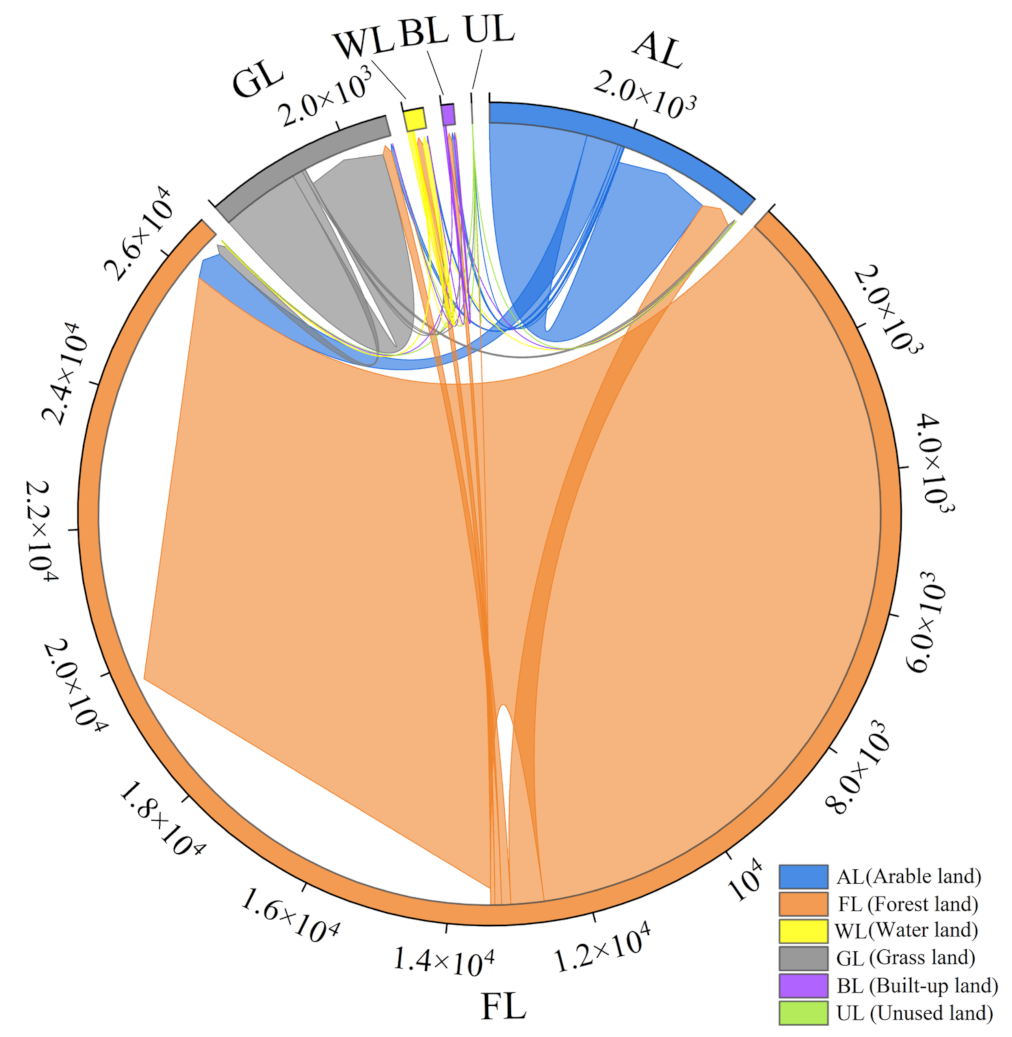
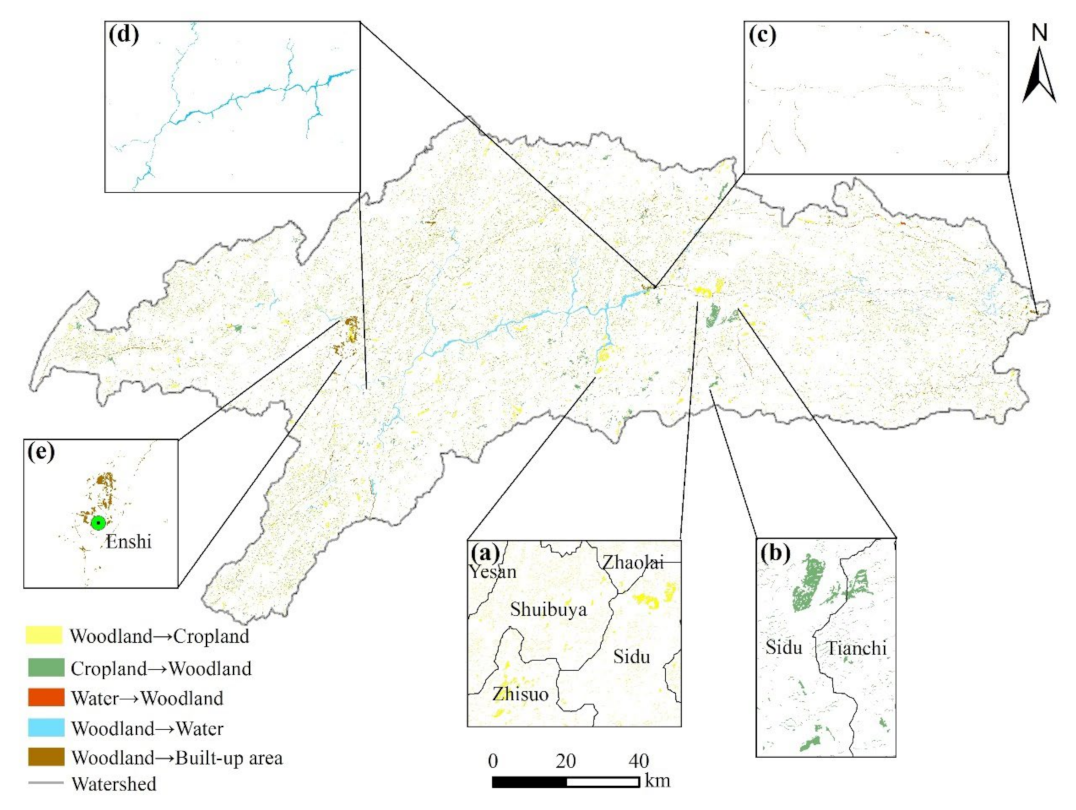
In the past 30 years, the area of cropland and woodland has decreased by 28.3 and 138.17 km², respectively, in the QJW, while the water and built-up land increased by 88.78 and 96.65 km², respectively. The land use transfer was insignificant before 2000, while the transfer was the greatest between 2000 and 2010. Before 2000, cultivated land was the main category of land transferred to water. After 2000, it became forest land, mainly resulting from the implementation of the water resource projects in the midstream and downstream of the QJW. Forest land was the main type transformed to built-up land, mainly concentrated in the center of Enshi City and on some major transportation roads.

(2)

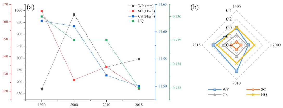
From 1990 to 2018, the WY increased by 18.92% in the QJW, while the SC, CS and HQ decreased by 26.94%, 1.05% and 0.4%, respectively. The increase in the arable land area led to an increase in WY. The decrease in forest land and the increase in construction land led to a decrease in SC, CS and HQ. Compared with SC, CS and HQ, the spatial distribution of WY varied more significantly over time. Except for LUCC in the QJW, meteorological and topographical factors had a great impact on WY and SC, respectively, while land use patterns greatly impacted CS and HQ.

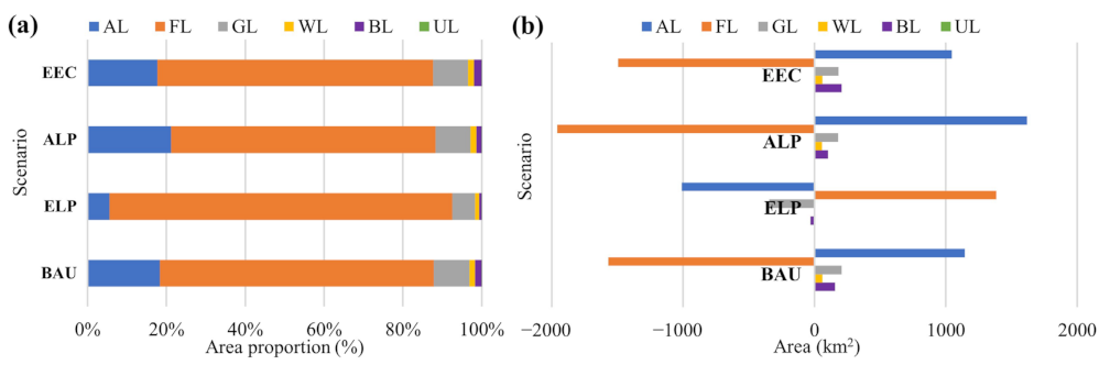
(3)

In 2034, there was predicted to be an apparent spatial conflict between the growth of arable land and the expansion of built-up land, especially in the area centered on the Lichuan, Enshi and Yidu counties of the QJW. The WY decreased significantly to the 700–721 mm range, while the SC, CS and HQ increased above 135 t·ha⁻¹, 13.6 t·ha⁻¹ and 0.8, respectively. The ranking of WY and SC values under four scenarios was ALP > BAU > EEC > ELP, while the ranking of CS and HQ was ELP > EEC > BAU > ALP. As the WY decreased significantly and the SC increased in 2034, the main ES of the QJW shifted from WY to SC. Considering the sustainable eco-socio-economic development of the QJW, the EEC scenario can be regarded as the future development scheme of the QJW compared with other scenarios.

(4)

Overall, with the protection of the Yangtze River as the premise, promoting overall ecological protection and creating financial industries integrating ecological tourism and agriculture can provide new ideas to achieve the sustainable development of the QJW. As the QJW is a complex ecosystem integrating nature, society and economy, the practical application should be combined with specific land use objectives and scenarios to select the appropriate land use pattern for the QJW. In the future, studies can consider further quantifying food production and energy supply functions of the QJW to establish a water–food–energy–ecosystem linkage framework, which can provide a deeper decision basis for the sustainable development of the region.

References

1. Costanza, R.; d’Arge, R.; De Groot, R.; Farber, S.; Grasso, M.; Hannon, B.; Limburg, K.; Naeem, S.; O’neill, R.V.; Paruelo, J. The value of the world’s ecosystem services and natural capital. Nature 1997, 387, 253–260. [Google Scholar] [CrossRef]
2. Wood, S.L.; Jones, S.K.; Johnson, J.A.; Brauman, K.A.; Chaplin-Kramer, R.; Fremier, A.; Girvetz, E.; Gordon, L.J.; Kappel, C.V.; Mandle, L. Distilling the role of ecosystem services in the Sustainable Development Goals. Ecosyst. Serv. 2018, 29, 70–82. [Google Scholar] [CrossRef]
3. Vitousek, P.M.; Aber, J.D.; Howarth, R.W.; Likens, G.E.; Matson, P.A.; Schindler, D.W.; Schlesinger, W.H.; Tilman, D.G. Human alteration of the global nitrogen cycle: Sources and consequences. Ecol. Appl. 1997, 7, 737–750. [Google Scholar] [CrossRef]
4. Millennium Ecosystem Assessment M. E. A. Ecosystems and Human Well-Being; Island Press: Washington, DC, USA, 2005; Volume 5.
5. Rodríguez, J.P.; Beard, T.D., Jr.; Bennett, E.M.; Cumming, G.S.; Cork, S.J.; Agard, J.; Dobson, A.P.; Peterson, G.D. Trade-offs across space, time, and ecosystem services. Ecol. Soc. 2006, 11, 28. [Google Scholar] [CrossRef]
6. Meacham, M.; Queiroz, C.; Norström, A.V.; Peterson, G.D. Social-ecological drivers of multiple ecosystem services: What variables explain patterns of ecosystem services across the Norrström drainage basin? Ecol. Soc. 2016, 21, 14. [Google Scholar] [CrossRef]
7. Reyers, B.; Biggs, R.; Cumming, G.S.; Elmqvist, T.; Hejnowicz, A.P.; Polasky, S. Getting the measure of ecosystem services: A social–ecological approach. Front. Ecol. Environ. 2013, 11, 268–273. [Google Scholar] [CrossRef]
8. Nagendra, H.; Mairota, P.; Marangi, C.; Lucas, R.; Dimopoulos, P.; Honrado, J.P.; Niphadkar, M.; Mücher, C.A.; Tomaselli, V.; Panitsa, M. Satellite Earth observation data to identify anthropogenic pressures in selected protected areas. Int. J. Appl. Earth Obs. Geoinf. 2015, 37, 124–132. [Google Scholar] [CrossRef]
9. Rimal, B.; Sharma, R.; Kunwar, R.; Keshtkar, H.; Stork, N.E.; Rijal, S.; Rahman, S.A.; Baral, H. Effects of land use and land cover change on ecosystem services in the Koshi River Basin, Eastern Nepal. Ecosyst. Serv. 2019, 38, 100963. [Google Scholar] [CrossRef]
10. Sannigrahi, S.; Zhang, Q.; Joshi, P.; Sutton, P.C.; Keesstra, S.; Roy, P.; Pilla, F.; Basu, B.; Wang, Y.; Jha, S. Examining effects of climate change and land use dynamic on biophysical and economic values of ecosystem services of a natural reserve region. J. Cleaner Prod. 2020, 257, 120424. [Google Scholar] [CrossRef]
11. Massad, R.S.; Lathière, J.; Strada, S.; Perrin, M.; Personne, E.; Stéfanon, M.; Stella, P.; Szopa, S.; de Noblet-Ducoudré, N. Reviews and syntheses: Influences of landscape structure and land uses on local to regional climate and air quality. Biogeosciences 2019, 16, 2369–2408. [Google Scholar] [CrossRef]
12. Wang, X.; Wu, J.; Liu, Y.; Hai, X.; Shanguan, Z.; Deng, L. Driving factors of ecosystem services and their spatiotemporal change assessment based on land use types in the Loess Plateau. J. Environ. Manag. 2022, 311, 114835. [Google Scholar] [CrossRef] [PubMed]
13. Asadolahi, Z.; Salmanmahiny, A.; Sakieh, Y.; Mirkarimi, S.H.; Baral, H.; Azimi, M. Dynamic trade-off analysis of multiple ecosystem services under land use change scenarios: Towards putting ecosystem services into planning in Iran. Ecol. Complexity 2018, 36, 250–260. [Google Scholar] [CrossRef]
14. He, J.; Shi, X.; Fu, Y.; Yuan, Y. Evaluation and simulation of the impact of land use change on ecosystem services trade-offs in ecological restoration areas, China. Land Use Pol. 2020, 99, 105020. [Google Scholar] [CrossRef]
15. Wang, Z.; Li, X.; Mao, Y.; Li, L.; Wang, X.; Lin, Q. Dynamic simulation of land use change and assessment of carbon storage based on climate change scenarios at the city level: A case study of Bortala, China. Ecol. Indic. 2022, 134, 108499. [Google Scholar] [CrossRef]
16. Gong, J.; Liu, D.; Zhang, J.; Xie, Y.; Cao, E.; Li, H. Tradeoffs/synergies of multiple ecosystem services based on land use simulation in a mountain-basin area, western China. Ecol. Indic. 2019, 99, 283–293. [Google Scholar] [CrossRef]
17. Xiang, S.; Wang, Y.; Deng, H.; Yang, C.; Wang, Z.; Gao, M. Response and multi-scenario prediction of carbon storage to land use/cover change in the main urban area of Chongqing, China. Ecol. Indic. 2022, 142, 109205. [Google Scholar] [CrossRef]
18. Li, Z.-T.; Li, M.; Xia, B.-C. Spatio-temporal dynamics of ecological security pattern of the Pearl River Delta urban agglomeration based on LUCC simulation. Ecol. Indic. 2020, 114, 106319. [Google Scholar] [CrossRef]
19. Wu, Z.; Zhou, R.; Zeng, Z. Identifying and Mapping the Responses of Ecosystem Services to Land Use Change in Rapidly Urbanizing Regions: A Case Study in Foshan City, China. Remote Sens. 2021, 13, 4374. [Google Scholar] [CrossRef]
20. Wang, P.; Li, R.; Liu, D.; Wu, Y. Dynamic characteristics and responses of ecosystem services under land use/land cover change scenarios in the Huangshui River Basin, China. Ecol. Indic. 2022, 144, 109539. [Google Scholar] [CrossRef]
21. Han, J.; Hu, Z.; Wang, P.; Yan, Z.; Li, G.; Zhang, Y.; Zhou, T. Spatio-temporal evolution and optimization analysis of ecosystem service value-A case study of coal resource-based city group in Shandong, China. J. Cleaner Prod. 2022, 363, 132602. [Google Scholar] [CrossRef]
22. Grêt-Regamey, A.; Brunner, S.H.; Kienast, F. Mountain ecosystem services: Who cares? Mt. Res. Dev. 2012, 32, S23–S34. [Google Scholar] [CrossRef]
23. Sun, X.; Shan, R.; Liu, F. Spatio-temporal quantification of patterns, trade-offs and synergies among multiple hydrological ecosystem services in different topographic basins. J. Cleaner Prod. 2020, 268, 122338. [Google Scholar] [CrossRef]
24. Cord, A.F.; Bartkowski, B.; Beckmann, M.; Dittrich, A.; Hermans-Neumann, K.; Kaim, A.; Lienhoop, N.; Locher-Krause, K.; Priess, J.; Schröter-Schlaack, C. Towards systematic analyses of ecosystem service trade-offs and synergies: Main concepts, methods and the road ahead. Ecosyst. Serv. 2017, 28, 264–272. [Google Scholar] [CrossRef]
25. Rajagopalan, P.; Lim, K.C.; Jamei, E. Urban heat island and wind flow characteristics of a tropical city. Sol. Energy 2014, 107, 159–170. [Google Scholar] [CrossRef]
26. Li, Z.; Deng, X.; Jin, G.; Mohmmed, A.; Arowolo, A.O. Tradeoffs between agricultural production and ecosystem services: A case study in Zhangye, Northwest China. Sci. Total Environ. 2020, 707, 136032. [Google Scholar] [CrossRef]
27. Droogers, P.; Allen, R.G. Estimating reference evapotranspiration under inaccurate data conditions. Irrig. Drain. Syst. 2002, 16, 33–45. [Google Scholar] [CrossRef]
28. Gupta, S.; Larson, W. Estimating soil water retention characteristics from particle size distribution, organic matter percent, and bulk density. Water Resour. Res. 1979, 15, 1633–1635. [Google Scholar] [CrossRef]
29. Sharp, R.; Douglass, J.; Wolny, S.; Arkema, K.; Bernhardt, J.; Bierbower, W.; Chaumont, N.; Denu, D.; Fisher, D.; Glowinski, K. InVEST 3.8.7. User’s Guide; The Natural Capital Project, Standford University, University of Minnesota, The Nature Conservancy, and World Wildlife Fund: Standford, CA, USA, 2020; pp. 20–40. [Google Scholar]
30. Zhang, C.; Li, W.; Zhang, B.; Liu, M. Water Yield of Xitiaoxi River Basin Based on InVEST Modeling. J. Resour. Ecol. 2012, 3, 50–54. [Google Scholar]
31. Allen, R.G.; Pereira, L.S.; Raes, D.; Smith, M. Crop Evapotranspiration-Guidelines for Computing Crop Water Requirements-FAO Irrigation and Drainage Paper 56; FAO: Rome, Italy, 1998; Volume 300, p. D05109. [Google Scholar]
32. Li, Q.; Zhou, Y.; Wang, L.; Zuo, Q.; Yi, S.; Liu, J.; Su, X.; Xu, T.; Jiang, Y. The Link between Landscape Characteristics and Soil Losses Rates over a Range of Spatiotemporal Scales: Hubei Province, China. Int. J. Environ. Res. Public Health 2021, 18, 11044. [Google Scholar] [CrossRef]
33. Borselli, L.; Cassi, P.; Torri, D. Prolegomena to sediment and flow connectivity in the landscape: A GIS and field numerical assessment. Catena 2008, 75, 268–277. [Google Scholar] [CrossRef]
34. Wischmeier, W.H.; Smith, D.D. Predicting Rainfall Erosion Losses: A Guide to Conservation Planning; Department of Agriculture, Science and Education Administration: Washington, DC, USA, 1978; pp. 5373–5377. [Google Scholar]
35. Zhang, K.; Peng, W.; Yang, H. Soil erodibility and its estimation for agricultural soil in China. Acta Pedol. Sin. 2007, 44, 7–13. [Google Scholar] [CrossRef]
36. Wang, P.; Zhang, L.; Li, Y.; Jiao, L.; Wang, H.; Yan, J.; Lü, Y.; Fu, B. Spatio-temporal characteristics of the trade-off and synergy relationships among multiple ecosystem services in the Upper Reaches of Hanjiang River Basin. Acta Geogr. Sin. 2017, 72, 2064–2078. [Google Scholar]
37. Cai, C.; Ding, S.; Shi, Z.; Huang, L.; Zhang, G. Study of applying USLE and geographical information system IDRISI to predict soil erosion in small watershed. J. Soil Water Conserv. 2000, 14, 19–24. [Google Scholar]
38. Chen, L.; Pei, S.; Liu, X.; Qiao, Q.; Liu, C. Mapping and analysing tradeoffs, synergies and losses among multiple ecosystem services across a transitional area in Beijing, China. Ecol. Indic. 2021, 123, 107329. [Google Scholar] [CrossRef]
39. Gong, J.; Cao, E.; Xie, Y.; Xu, C.; Li, H.; Yan, L. Integrating ecosystem services and landscape ecological risk into adaptive management: Insights from a western mountain-basin area, China. J. Environ. Manag. 2021, 281, 111817. [Google Scholar] [CrossRef]
40. Chuai, X.; Huang, X.; Lai, L.; Wang, W.; Peng, J.; Zhao, R. Land use structure optimization based on carbon storage in several regional terrestrial ecosystems across China. Environ. Sci. Policy 2013, 25, 50–61. [Google Scholar] [CrossRef]
41. Wang, C.; Zhan, J.; Chu, X.; Liu, W.; Zhang, F. Variation in ecosystem services with rapid urbanization: A study of carbon sequestration in the Beijing–Tianjin–Hebei region, China. Phys. Chem. Earth Parts A/B/C 2019, 110, 195–202. [Google Scholar] [CrossRef]
42. Hall, L.S.; Krausman, P.R.; Morrison, M.L. The habitat concept and a plea for standard terminology. Wildl. Soc. Bull. 1997, 25, 173–182. [Google Scholar]
43. Liu, Y.; Zhou, Y.; Du, Y. Study on the spatio-temporal patterns of habitat quality and its terrain gradient effects of the middle of the Yangtze River Economic Belt based on InVEST model. Resour. Environ. Yangtze Basin 2019, 28, 2429–2440. [Google Scholar]
44. Gong, J.; Xie, Y.; Cao, E.; Huang, Q.; Li, H. Integration of InVEST-habitat quality model with landscape pattern indexes to assess mountain plant biodiversity change: A case study of Bailongjiang watershed in Gansu Province. J. Geog. Sci. 2019, 29, 1193–1210. [Google Scholar] [CrossRef]
45. Singh, S.K.; Mustak, S.; Srivastava, P.K.; Szabó, S.; Islam, T. Predicting spatial and decadal LULC changes through cellular automata Markov chain models using earth observation datasets and geo-information. Environ. Process. 2015, 2, 61–78. [Google Scholar] [CrossRef]
46. Chen, Y.; Li, X.; Liu, X.; Ai, B. Modeling urban land-use dynamics in a fast developing city using the modified logistic cellular automaton with a patch-based simulation strategy. Int. J. Geog. Inf. Sci. 2014, 28, 234–255. [Google Scholar] [CrossRef]
47. He, D.; Jin, F.; Zhou, J. The changes of land use and landscape pattern based on Logistic-CA-Markov Model—A case study of Beijing-Tianjin-Hebei metropolitan region. Sci. Geogr. Sin. 2011, 31, 903–910. [Google Scholar]
48. Yeh, A.G.-O.; Li, X. A constrained CA model for the simulation and planning of sustainable urban forms by using GIS. Environ. Plan. B Plan. Des. 2001, 28, 733–753. [Google Scholar] [CrossRef]
49. Wu, W.; Peng, J.; Liu, Y.; Hu, Y. Trade-off and synergy analysis of ecosystem services in Erdos City. Adv. Geosci. 2017, 36, 1571–1581. [Google Scholar]
50. Wang, J.F.; Li, X.H.; Christakos, G.; Liao, Y.L.; Zhang, T.; Gu, X.; Zheng, X.Y. Geographical detectors-based health risk assessment and its application in the neural tube defects study of the Heshun Region, China. Int. J. Geog. Inf. Sci. 2010, 24, 107–127. [Google Scholar] [CrossRef]
51. Huo, H.; Sun, C. Spatiotemporal variation and influencing factors of vegetation dynamics based on Geodetector: A case study of the northwestern Yunnan Plateau, China. Ecol. Indic. 2021, 130, 108005. [Google Scholar] [CrossRef]
52. Li, B.; Pan, B.; Han, J. Basic terrestrial geomorphological types in China and their circumscriptions. Quat. Sci. 2008, 28, 535–543. [Google Scholar]
53. Xue, C.; Chen, X.; Xue, L.; Zhang, H.; Chen, J.; Li, D. Modeling the spatially heterogeneous relationships between tradeoffs and synergies among ecosystem services and potential drivers considering geographic scale in Bairin Left Banner, China. Sci. Total Environ. 2023, 855, 158834. [Google Scholar] [CrossRef]
54. Fotheringham, A.S.; Yang, W.; Kang, W. Multiscale geographically weighted regression (MGWR). Ann. Am. Assoc. Geogr. 2017, 107, 1247–1265. [Google Scholar] [CrossRef]
55. Wu, T.; Zhou, L.; Jiang, G.; Meadows, M.E.; Zhang, J.; Pu, L.; Wu, C.; Xie, X. Modelling spatial heterogeneity in the effects of natural and socioeconomic factors, and their interactions, on atmospheric pm2. 5 concentrations in china from 2000–2015. Remote Sens. 2021, 13, 2152. [Google Scholar] [CrossRef]
56. Wei, P.; Xie, S.; Huang, L.; Liu, L. Ingestion of GNSS-Derived ZTD and PWV for spatial interpolation of PM2.5 concentration in Central and Southern China. Int. J. Environ. Res. Public Health 2021, 18, 7931. [Google Scholar] [CrossRef] [PubMed]
57. Mollalo, A.; Vahedi, B.; Rivera, K.M. GIS-based spatial modeling of COVID-19 incidence rate in the continental United States. Sci. Total Environ. 2020, 728, 138884. [Google Scholar] [CrossRef] [PubMed]
58. Oshan, T.M.; Smith, J.P.; Fotheringham, A.S. Targeting the spatial context of obesity determinants via multiscale geographically weighted regression. Int. J. Health Geogr. 2020, 19, 11. [Google Scholar] [CrossRef]
59. Iyanda, A.E.; Osayomi, T. Is there a relationship between economic indicators and road fatalities in Texas? A multiscale geographically weighted regression analysis. GeoJournal 2021, 86, 2787–2807. [Google Scholar] [CrossRef]
60. Rong, Y.; Li, K.; Guo, J.; Zheng, L.; Luo, Y.; Yan, Y.; Wang, C.; Zhao, C.; Shang, X.; Wang, Z. Multi-scale spatio-temporal analysis of soil conservation service based on MGWR model: A case of Beijing-Tianjin-Hebei, China. Ecol. Indic. 2022, 139, 108946. [Google Scholar] [CrossRef]
61. Clerici, N.; Cote-Navarro, F.; Escobedo, F.J.; Rubiano, K.; Villegas, J.C. Spatio-temporal and cumulative effects of land use-land cover and climate change on two ecosystem services in the Colombian Andes. Sci. Total Environ. 2019, 685, 1181–1192. [Google Scholar] [CrossRef]
62. Guo, M.; Ma, S.; Wang, L.-J.; Lin, C. Impacts of future climate change and different management scenarios on water-related ecosystem services: A case study in the Jianghuai ecological economic Zone, China. Ecol. Indic. 2021, 127, 107732. [Google Scholar] [CrossRef]
63. Lang, Y.; Song, W.; Zhang, Y. Responses of the water-yield ecosystem service to climate and land use change in Sancha River Basin, China. Phys. Chem. Earth Parts A/B/C 2017, 101, 102–111. [Google Scholar] [CrossRef]
64. Gao, J.; Bian, H.; Zhu, C.; Tang, S. The response of key ecosystem services to land use and climate change in Chongqing: Time, space, and altitude. J. Geog. Sci. 2022, 32, 317–332. [Google Scholar] [CrossRef]
65. Liu, X.; Pei, F.; Wen, Y.; Li, X.; Wang, S.; Wu, C.; Cai, Y.; Wu, J.; Chen, J.; Feng, K. Global urban expansion offsets climate-driven increases in terrestrial net primary productivity. Nat. Commun. 2019, 10, 5558. [Google Scholar] [CrossRef] [PubMed]
66. Sun, X.; Li, F. Spatiotemporal assessment and trade-offs of multiple ecosystem services based on land use changes in Zengcheng, China. Sci. Total Environ. 2017, 609, 1569–1581. [Google Scholar] [CrossRef]
67. Wu, J. Landscape sustainability science (II): Core questions and key approaches. Landscape Ecol. 2021, 36, 2453–2485. [Google Scholar] [CrossRef]
68. Zuo, Q.; Zhou, Y.; Wang, L.; Li, Q.; Liu, J. Impacts of future land use changes on land use conflicts based on multiple scenarios in the central mountain region, China. Ecol. Indic. 2022, 137, 108743. [Google Scholar] [CrossRef]
69. Wang, Z.; Zeng, J.; Chen, W. Impact of urban expansion on carbon storage under multi-scenario simulations in Wuhan, China. Environ. Sci. Pollut. Res. 2022, 29, 45507–45526. [Google Scholar] [CrossRef]
70. Wen, X.; Théau, J. Spatiotemporal analysis of water-related ecosystem services under ecological restoration scenarios: A case study in northern Shaanxi, China. Sci. Total Environ. 2020, 720, 137477. [Google Scholar] [CrossRef] [PubMed]
71. Hou, Y.; Burkhard, B.; Müller, F. Uncertainties in landscape analysis and ecosystem service assessment. J. Environ. Manag. 2013, 127, S117–S131. [Google Scholar] [CrossRef] [PubMed]
Figure 1. The geographical location of the Qingjiang Watershed.
Remotesensing 15 02759 g001
Figure 2. Area statistics of land use/cover change in the Qingjiang Watershed from 1990 to 2018: (a) Comparison of area proportion of six land use types in 1990, 2000, 2010 and 2018; (b) composition proportion of six land use types in 1990, 2000, 2010 and 2018; (c) transfer area of land use types from 1990 to 2018.
Remotesensing 15 02759 g002
Figure 3. Transfer area of six land use types in the Qingjiang Watershed from 1990 to 2018 (km2).
Remotesensing 15 02759 g003
Figure 4. Spatial distribution of the main land use transfer in the Qingjiang Watershed: (a) woodland converted to cropland; (b) cropland converted to woodland; (c) water converted to woodland; (d) woodland converted to water; (e) woodland converted to built-up area.
Remotesensing 15 02759 g004
Figure 5. Temporal analysis of ES changes from 1990 to 2018: (a) Temporal change of ESs; (b) radar map of standardized ESs.
Remotesensing 15 02759 g005
Figure 6. Spatial patterns of four ESs in the Qingjiang Watershed from 1990 to 2018.
Remotesensing 15 02759 g006
Figure 7. The changes of four ESs in three land use types in the Qingjiang Watershed from 1990 to 2018.
Remotesensing 15 02759 g007
Figure 8. The quantitative effects of arable land (AL) area and forest land (FL) area in depicting four ESs in the Qingjiang Watershed in 2018.
Remotesensing 15 02759 g008
Figure 9. Area statistics of land use/cover change in the Qingjiang Watershed in 2034: (a) Composition proportion of six land use types under four scenarios; (b) transfer area of land use types under four scenarios from 2018 to 2034.
Remotesensing 15 02759 g009
Figure 10. Spatial patterns of land use/cover in the Qingjiang Watershed in 2034.
Remotesensing 15 02759 g010
Figure 11. Temporal analysis of ES change in 2034: (a) Temporal change of ESs; (b) Radar map of standardized ESs.
Remotesensing 15 02759 g011
Figure 12. Spatial patterns of four ESs in the Qingjiang Watershed in 2034.
Remotesensing 15 02759 g012
Figure 13. The changes of four ESs in three land use types in the Qingjiang Watershed in 2034.
Remotesensing 15 02759 g013
Figure 14. The results of geodetector for four ESs in the Qingjiang Watershed in 2018: (a) The q values of the factor detector for four ESs; (b) the q values of the interaction detector for four ESs.
Remotesensing 15 02759 g014