The Importance of Spatial Resolution in the Modeling of Methane Emissions from Natural Wetlands

Abstract

An important uncertainty in the modeling of methane (CH₄) emissions from natural wetlands is the wetland area. It is difficult to model wetlands’ CH₄ emissions because of several factors, including its spatial heterogeneity on a large range of scales. In this study, we investigate the impact of model resolution on the simulated wetland methane emission for the Fennoscandinavian Peninsula. This is carried out using a high-resolution wetland map (100 × 100 m²) and soil carbon map (250 × 250 m²) in combination with a highly simplified CH₄ emission model that is coarsened in five steps from 0.005° to 1°. We find a strong relation between wetland emissions and resolution, which is sensitive, however, to the sub-grid treatment of the wetland fraction. In our setup, soil carbon and soil moisture are positively correlated at a high resolution, with the wetland location leading to increasing CH₄ emissions with increasing resolution. Keeping track of the wetland fraction reduces the impact of resolution. However, uncertainties in CH₄ emissions remain high because of the large uncertainty in the representation of wetland the area, as demonstrated using the output of the WetChimp intercomparison over our study domain. Because of wetland mapping uncertainties, existing models are unlikely to realistically represent the correlation between soil moisture and soil carbon availability. The correlation is positive in our simplified model but may be different in more complex models depending on their method of representing substrate availability. Therefore, depending on the correlation, CH₄ emissions may be over- or underestimated. As increasing the model resolution is an effective approach to mitigate the problem of accounting for the correlation between soil moisture and soil carbon and to improve the accuracy of models, the main message of this study is that increasing the resolution of global wetland models, and especially the input datasets that are used, should receive high priority.

1. Introduction

Despite decades of research, the main drivers of variations in the growth rate of atmospheric methane (CH₄) are still poorly understood [1]. This is a critical knowledge gap, since CH₄ is the second most important anthropogenic greenhouse gas after carbon dioxide (CO₂) [2], and the increase in its recent growth rate introduces significant uncertainty in the scenarios that are used in climate projections [3,4]. While those projections are mainly concerned with anthropogenic emissions, natural emissions of CH₄ are also important since they account for an important fraction of the growth rate uncertainty [1,5]. This can be explained by the poorly quantified response of these emissions to changing climatological conditions on a wide range of temporal and spatial scales [5].

Natural wetlands have by far the largest contribution to the natural budget of methane estimated at 145 Tg CH₄ yr⁻¹, accounting for 20–40% of total global CH₄ emissions [1]. Generally, natural wetlands are defined as ecosystems with intermittent or permanent water-saturated soils, such as peatlands (bogs and fens), mineral soil wetlands (swamps and marshes), determining the vegetation composition, productivity, and nutrient cycling [1]. Due to their nature, wetlands are carbon-rich and moist environments favorable to microbes metabolizing organic matter under anaerobic conditions leading to CH₄ production [6]. Estimates of CH₄ emissions from wetlands using a range of top-down and bottom-up techniques show a large inconsistency between the two approaches [1], resulting from large uncertainties in the distribution and the underlying processes controlling the balance between microbial production and oxidation of methane [7,8].

Models used for quantifying CH₄ emissions vary in their methodology and level of detail. The WetChimp model inter-comparison [8] highlighted the variety of models that are used and the wide range of global and regional emissions resulting from them. The global distribution and area of wetlands, determined either using wetland maps, hydrological modeling, or satellite-derived inundation maps, was identified as a main source of uncertainty [8,9]. It was concluded that the simulated wetland extents are difficult to evaluate due to extensive disagreements between remotely sensed inundation datasets and wetland mapping [9]. The simulated global wetlands’ CH₄ flux estimates were in the range of 141 to 264 Tg CH₄ yr⁻¹ with a mean value of 190 Tg CH₄ yr⁻¹ [9], which is in the upper part of the large uncertainty range of the early estimate by Reference [10] of 10 to 300 Tg CH₄ yr⁻¹. Despite the progress in narrowing that range, the uncertainty in global wetland CH₄ emissions remains very high [9].

The recent global CH₄ budget study in Reference [1] compared 13 models for the 2008–2017 period, resulting in somewhat lower global emissions in the range of 101 and 179 Tg CH₄ yr⁻¹ with an average of 148 Tg CH₄ yr⁻¹. Again, it was concluded that wetland extent appears to be the main contributor to uncertainties in the absolute flux of CH₄ emissions from wetlands, as well as in other recent studies on this topic [4,11,12]. Ref. [13] concluded that it is an important need for the scientific community to construct a global-scale wetland dataset at high spatial and temporal resolution, by integrating multiple sources of field and satellite data using models.

Reference [14] investigated the sensitivity of CH₄ emissions from pan-arctic wetlands to the spatial resolution of water table depth, comparing simulations at 5 and 100 km resolution. The significant differences that were found suggest that macro-scale biogeochemical models using grid-cell-mean water table depth might have underestimated the regional CH₄ emissions. It was recommended to consider the spatial scale dependence of CH₄ emissions on water table depth in future quantifications. Reference [15] examined the influence of spatial resolution and land-cover heterogeneity on the accuracy of land-cover mapping. It was concluded that spatial resolution plays an important role in classifying land cover. The fraction of mixed ecosystem pixels decreased, and the overall classification accuracy improved when the spatial resolution was increased.

In this study, we investigate the importance of spatial resolution for the quantification of methane emissions from natural wetlands and whether the use of high-resolution wetland maps may be an effective strategy for reducing its uncertainty. The sensitivity of emissions to spatial resolution is tested for the Fennoscandinavian domain, using a high-resolution wetland map (100 × 100 m²) in combination with a highly simplified CH₄ emission model. The advantage of using a simple model is its numerical efficiency as well as the conceptual ease to control and understand the relations that are found. The wetland map is coarsened across a wide range of resolutions, including those that are commonly used in global wetland models. Site measurements from Finland are used to calibrate the model before it is used to compute the impact of resolution on the integrated CH₄ emission over the study area. Finally, wetland extent maps from the WetChimp models intercomparison inventory are used to assess the significance and realism of the results obtained using the simple model.

2. Materials and Methods

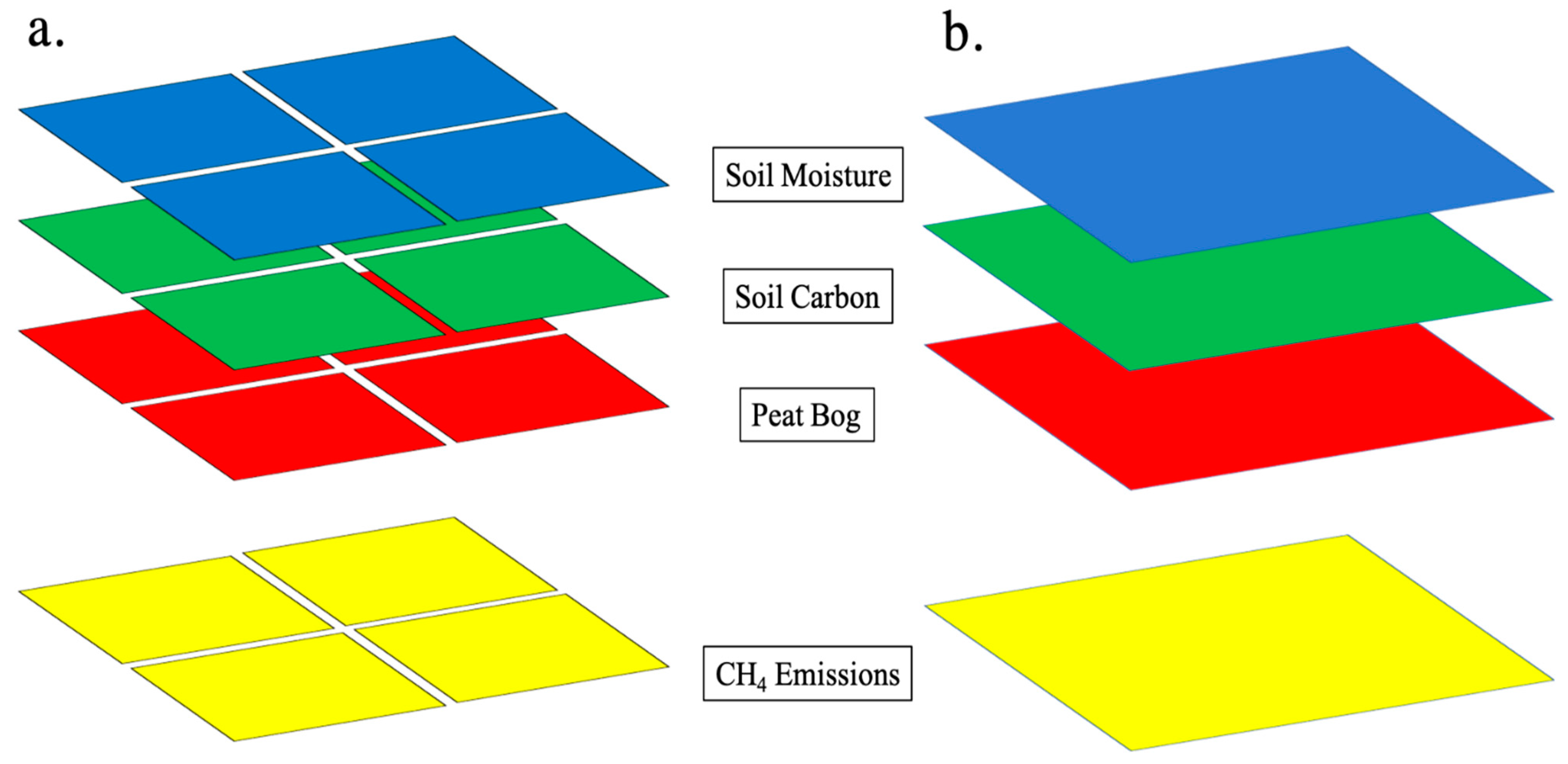
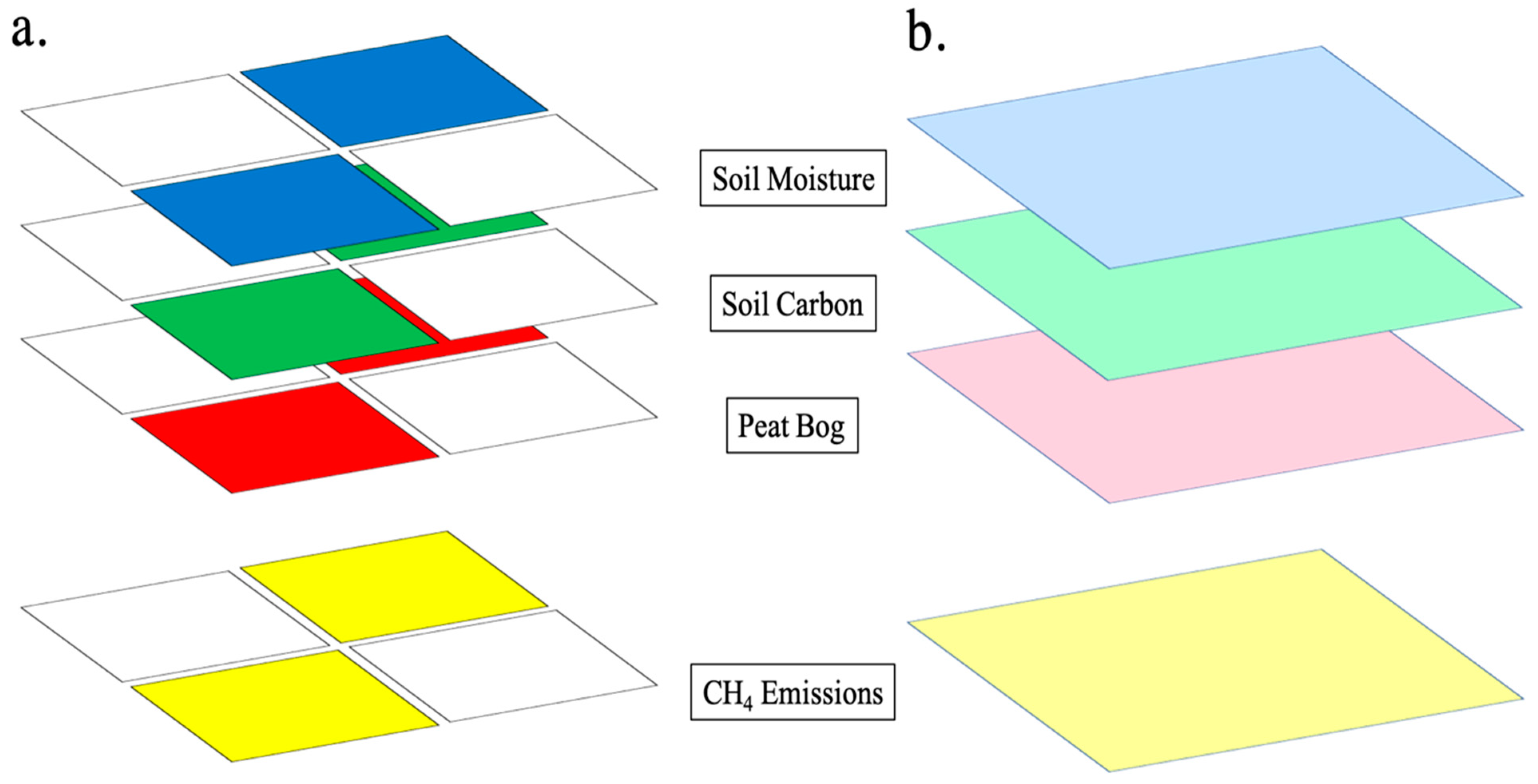
2.1. Hypothetical Experiment

The principle of the resolution dependence we investigate can be explained using a simple hypothetical case. Let us assume a wetland area W that can be described either at high resolution by 2 × 2 tiles, each with area A_T = 1, or at low resolution by combining the 2 × 2 tiles into a single tile of A_T = 4 (see Figure 1). To quantify the CH₄ emissions in these tiles, we use the highly simplified model of wetland emissions,

$${FCH}_4=SOC.SM.A_T$$

(1)

in which the CH₄ emission (F_CH4) is the product of the availability of soil carbon (SOC), soil moisture (SM), and the area of each wetland tile (A_T). This model is a simplified version of CH₄ emission equation that we will use in the remainder of this study, as will be explained in Section 2.2.

In the first case, we set SOC and SM both to unity. As a result, in the high-resolution representation (Figure 1a), each cell has an emission of 1, and therefore the total emission over wetland area W equals 4 (in arbitrary units). When aggregating the high-resolution tiles to coarse resolution (Figure 1b), soil moisture and soil carbon are the average of the 2 × 2 tiles. In this case, the sum of emissions will again be 4, i.e., the high- and low-resolution representations are consistent.

Alternatively, we assume that wetlands are located in two cells only (Figure 2a), the other two cells being upland. For upland tiles, we assume soil carbon and soil moisture to be zero, so wetland CH₄ emissions are also zero. Then, when applying the same principle, the total emission in the high-resolution case is 2 (Figure 2a), whereas it is 1 (4 × 0.5 × 0.5) in the low-resolution case (Figure 2b). Here, the resolution-dependence of the CH₄ emission arises because of the product SOC × SM in Equation (1), causing the impact of the averaging to coarse resolution on the CH₄ emission to be squared.

This outcome can be generalized to larger steps in resolution as follows:

$$E_{LR}=\overline{SOC}.\overline{SM}.A_{LR}={(n}_{wl}{SOC}_{wl}{A_{HR}/A_{LR}\left)\right(n_{wl}SM}_{wl}{A}_{HR}/A_{LR})A_{LR}$$

(2)

$$E_{HR}={n_{wl}SOC}_{wl}S{M}_{wl}{A}_{HR}$$

(3)

$$\frac{E_{HR}}{E_{LR}}=\frac{{n_{wl}SOC}_{wl}{SM}_{wl}{A}_{HR}}{{(n}_{wl}{SOC}_{wl}{A_{HR}/A_{LR}\left)\right(n_{wl}SM}_{wl}{A}_{HR}/A_{LR})A_{LR}}=\frac{A_{LR}}{n_{wl}{A}_{HR}}=\frac{1}{F_{wl}}$$

(4)

where E_HR and E_LR are the emissions of the coarse-resolution grid box evaluated at, respectively, high and low resolution.

A_HR and A_LR are the grid box areas at high and low resolution, respectively, and n_wl is the number of high-resolution grid boxes that are covered by wetland (note the use of the subscript wl to indicate a wetland grid box). If F_wl is the wetland fraction, then the right-hand-side term in Equation (4) is 1/F_wl. As long as the wetland fraction remains the same, the impact of a change in resolution will also remain the same. However, if the wetland fraction becomes lower, because part of the coarse-resolution wetland grid box happens to be dry at high resolution, then the impact of a change in resolution increases.

2.2. Wetlands CH₄ Model

The CH₄ emission scheme of Gendey et al. [16] is used to compute CH₄ emissions for the case study area described in Section 2.1. It is a highly simplified representation of wetland CH₄ emissions but is well suited for testing resolution dependences because of its computational efficiency and ease of interpretation as the number of model parameters is small. The CH₄ flux from wetlands F_CH4 (g CH₄ m⁻² yr⁻¹) is calculated from the basic CH₄ controls of soil temperature (T_soil), soil moisture (SM), and soil organic carbon (SOC), as follows:

$$F_{CH4}=K_{CH4}.SOC.SM.{Q_{10}}^{\raisebox{1ex}{$({\mathrm{T}}_{\mathrm{soil}}-{\mathrm{T}}_0)$}\!\left/ \!\raisebox{-1ex}{$10$}\right.}$$

(5)

where T_soil is the average soil surface temperature in Kelvin (K) for the top 5 cm. Q₁₀ is the temperature sensitivity of the CH₄ emission to a 10 K temperature change relative to T₀ = 273.15 K. Since F_CH4 is now expressed as the CH₄ flux per unit area, this is also used for soil carbon (SOC in (g.m⁻²)). K_CH4 is a calibration constant relating the driving variables to a CH₄ flux in units of (g CH₄ m⁻² yr⁻¹). We want to note here that the input data used in Equation (5) are for the year 2015, as will be described in Section 2.4.

Different scenarios are used (Sn.1–Sn.4) representing wetlands, uplands, and combinations between them (

Table 1. List of Scenarios.

Scenarios	Wetlands		Uplands		Temperature (K)
	SOC (g.m−2)	SM (cm3.cm−3)	SOC (g.m−2)	SM (cm3.cm−3)
Sn.1	ISRIC 2017	0.70	ISRIC 2017	0	ERA5
Sn.2	ISRIC 2017	0	ISRIC 2017	0.25	ERA5
Sn.3	ISRIC 2017	0.70	ISRIC 2017	0.25	ERA5
Sn.4-a	ISRIC 2017	ERA5	ISRIC 2017	0	ERA5
Sn.4-b	ISRIC 2017	PCRG	ISRIC 2017	0	ERA5

). In Sn.1, we use the high-resolution wetlands map (see Section 2.4.1) as a mask for wetlands to distinguish wetlands from the upland surroundings. CH₄ emissions are only calculated for the wetland fraction F_wl. This is because Equation (5) does not apply to aerobic upland soils, where CH₄ oxidation by methanotrophic bacteria dominates methanogenic CH₄ production.

However, in Sn.2, uplands are treated as the wetlands in Sn.1. CH₄ oxidation in upland soils may also show a resolution dependence following the logic of Section 2.1. However, since the upland fraction is generally substantially larger than the wetland fraction at spatial resolutions that are common in global wetland modeling, the sensitivity of the sink to resolution is expected to be less important (see Equation (4)). The setup of Sn.2 is meant to isolate the impact of the difference between the wetland and upland fraction on the resolution dependence, which explains why the method to compute the flux is kept the same. Sn.3 combines wetlands and uplands to test the impact of changing the contrast between upland and wetland emissions using the same threshold values of SOC and SM in Sn.1 and Sn.2. Sn.4 represents emissions from wetlands only, like in Sn.1, but using spatially varying SM and SOC data (Section 2.4). The aim is to test the extent to which the results of Sn.1 and Sn.2 might have been influenced by the simplifying assumptions on SOC and SM that are made, and how sensitive the resolution dependence may be to a more realistic representation of their spatial variations.

The first three scenarios used to test the resolution dependence were aggregated from the original high-resolution wetlands datasets described in the data section at 5 different resolutions; 0.01°, 0.05°, 0.1°, 0.5°, and 1°. For the remaining scenario, we aggregated from the finest available resolution of the ERA5 and PCRG soil moisture to 0.1°, 0.5°, and 1°.

We acknowledge that our wetland “model” provides only a highly simplified representation of the processes controlling CH₄ emissions in wetlands. However, the main objective is to demonstrate the principle and provide a first-order estimate of its importance, suitable to provide a basic discussion to be refined further using more sophisticated models in the future.

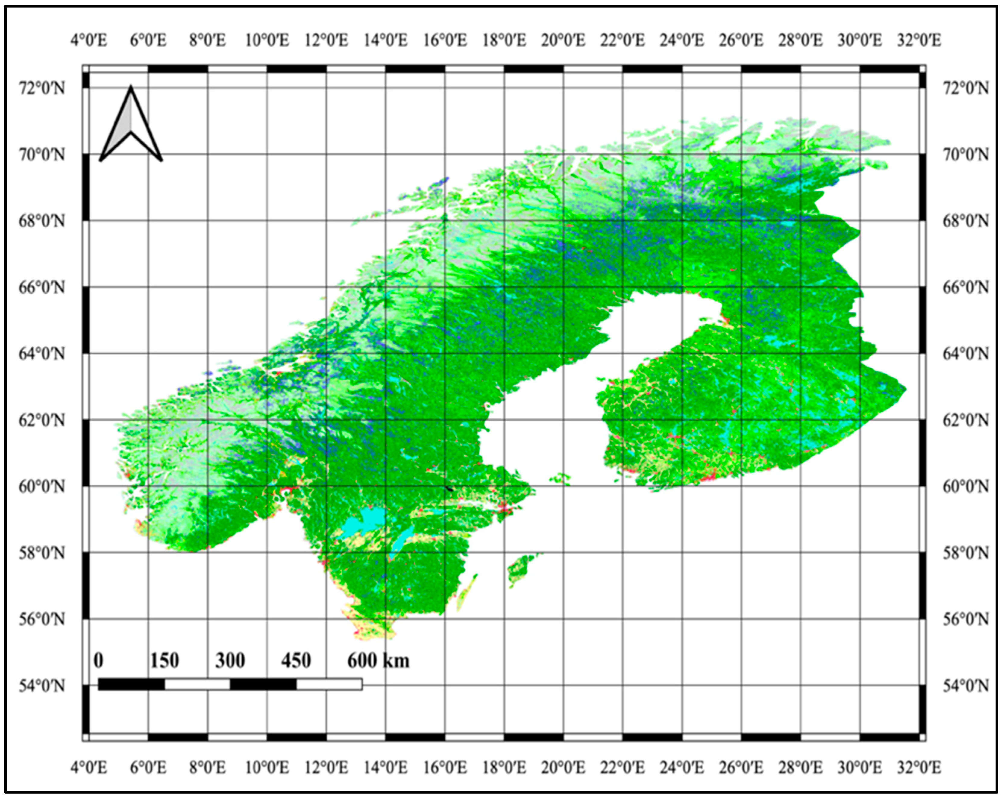
2.3. Study Area and Data

Study Area

The Fennoscandinavian peninsula, excluding the Russian sector, is used as the domain of our computations (see Figure 3). It is chosen as a favorable compromise between size, importance of high-latitude CH₄ emissions, ecosystem diversity, and data availability. In this domain, CH₄ fluxes are monitored at a few sites that are reporting to FLUXNET-CH₄ (https://fluxnet.org) (accessed on 23 January 2019). Despite the limited number of sites (2 sites in this study), the network density is still relatively high for the circumpolar boreal/arctic region.

2.4. Data

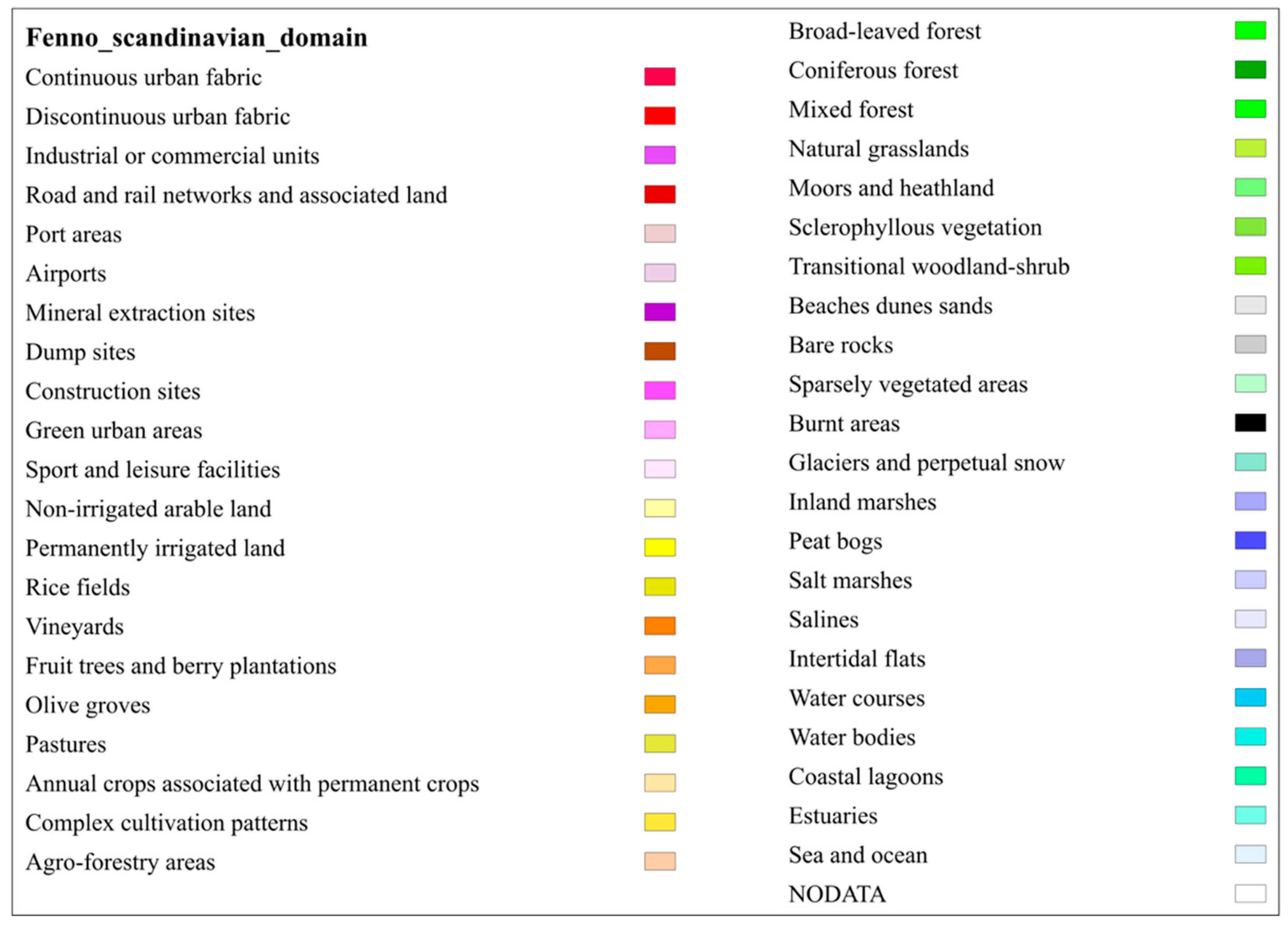
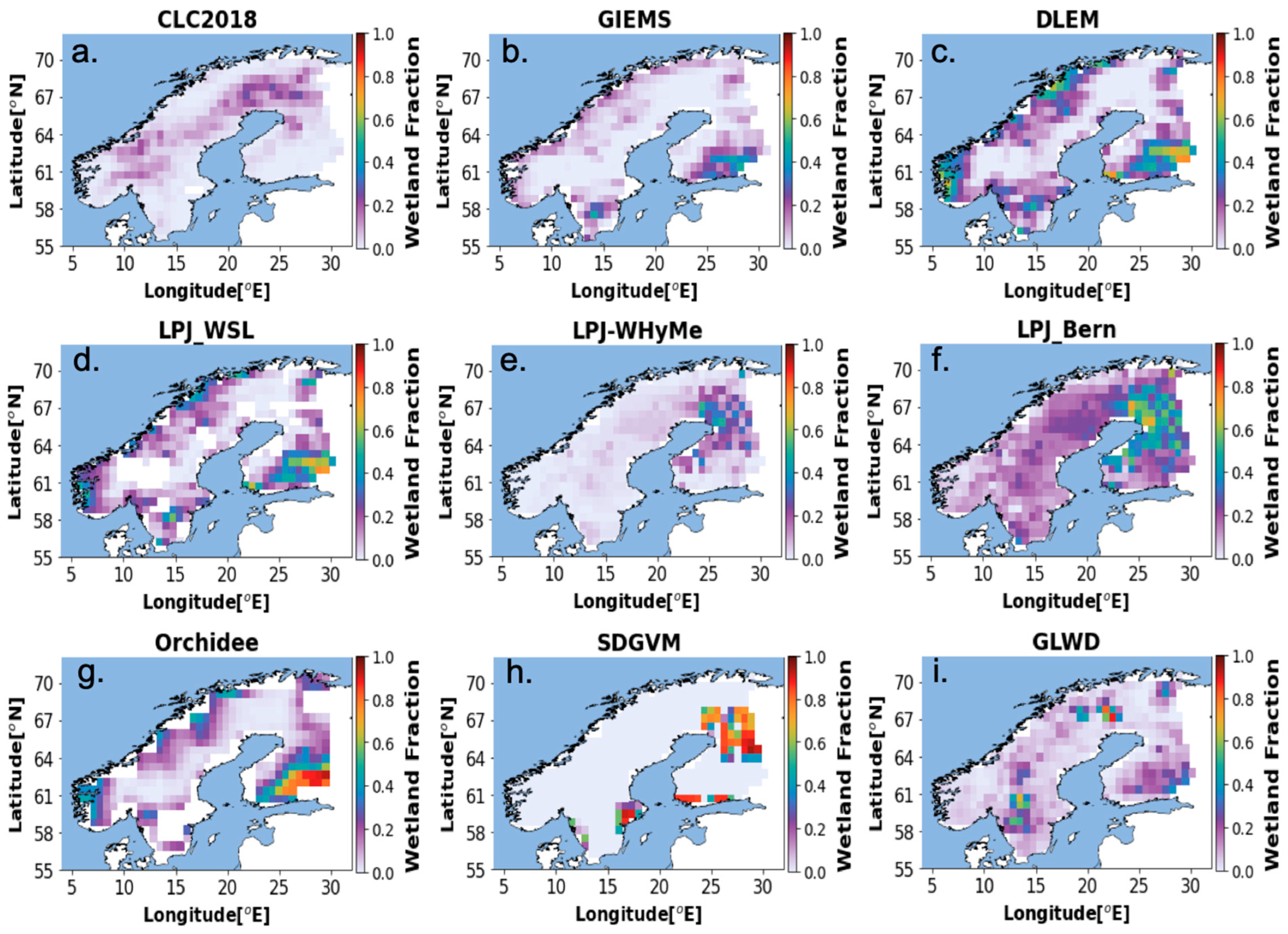
2.4.1. Wetland Map

To localize wetlands at a high resolution, the Corine Land Cover map is used (CLC2018). These data are made available by the Copernicus Land Monitoring Service from (https://land.copernicus.eu/pan-european/corine-land-cover/clc2018) (accessed on 12 March 2019). CLC2018 resolution is in order of sub-kilometers (100 × 100 m² = 0.001°) for the European continent [17] and provides information about the physical state of the landscape [18]. The land-cover classification is based on satellite images with a spatial resolution in the order of meters, from sensors onboard Landsat, RapidEye, Sentinel-2, and Landsat-8. This information is extended using various auxiliary data, e.g., aerial photographs, thematic maps, etc., yielding a high-resolution land cover map suitable for large -scale research and land cover/use mapping [18]. CLC2018 classifies wetlands into major categories: inland wetlands and coastal wetlands. Inland wetlands are inland marches and peatbogs (class numbers 411 and 412, respectively), which we use in our study as described in the CLC2018 user guide [19]. The CLC2018 map afterwards aggregated to 0.005° resolution, as will be known afterward as “reference resolution”.

2.4.2. Organic Soil Carbon SOC

To specify SOC in Equation (2), the soil carbon dataset from the International Soil Reference and Information Centre [20] at 250 × 250 m resolution is used. According to the ISRIC map, the SOC for the study area ranges between (10–110 g.m⁻²). The ISRIC data were downloaded from (https://files.isric.org/soilgrids/former/2017-03-10/data) (accessed on 2 March 2019). The SOC map was aggregated to 0.005° resolution to match the reference resolution benchmark.

2.4.3. Soil Moisture SM

The study by Reference [21] hypothesized that CH₄ fluxes peak at a soil moisture between 30% and 70% of water-filled pore space and declines below 20% and above 80% to assess the influence of soil temperature and soil moisture on CH₄ fluxes. Following this hypothesis, for Sn.1 and Sn.3, we used an average SM for uplands of 0.25 cm³.cm⁻³ again as an attempt to lower the impact of upland resolution dependence when following the coarsening steps explained in the following subsection. SM was maximized at wetlands locations to be 0.70 cm³.cm⁻³.

For Sn.4-a, we used ERA5 soil moisture, which is the most modern reanalysis product from the European Centre for Medium-Range Weather Forecasts (ECMWF) dataset for the top 7 cm soil layer for the year 2015 [22]. ERA5 combines large quantities of historical observations into the global land variable estimates, using the latest ECMWF modeling and data assimilation techniques. The ERA5 data coverage period starts from 1981 to 2–3 months before the present time, while the preliminary data update the dataset that is available within 5 days of real time. The ERA5 SM datasets are aggregated to 0.1°, 0.5°, and 1° resolution.

To test the robustness of the choice of SM dataset (Sn.4-b), we used another SM dataset from PCR-GLOBWB (PCRG), a grid-based global hydrology and water resources model developed by a group of scientists at the department of physical geography, Utrecht University, The Netherlands [23]. We ran the model to simulate SM for the study area using the finest resolution version with spatial resolutions of 5 arcmin (≈10 km). PCRG has three different soil depth layers, 0–5 cm (top layer), 5–30 cm, and 30–150 cm. A simulation was carried out for the year 2015 and output was used for the top 5 cm soil layer after remapping the data to 0.1°, 0.5°, and 1° resolutions.

2.4.4. Temperature T

The temperature in Equation (5) was taken from ERA5, using daily soil surface temperature for the top 5 cm of the soil for the year 2015. Data at a spatial resolution of 7 × 7 km² were downloaded from (https://www.ecmwf.int/en/forecasts/datasets/reanalysis-datasets/era5) (accessed on 4 June 2019). We acknowledge that this resolution should preferably have been higher. Although air temperature variations may be represented adequately enough at this resolution, the surface energy balance of wetlands and upland ecosystems is expected to be different. This gives rise to variations in soil surface temperature that we are unable to account for but are assumed to be of second order in importance compared to variations in soil carbon and soil moisture.

2.4.5. Q₁₀ and KCH₄

For the temperature sensitivity of methane emissions from natural wetlands, previous studies derived Q₁₀ values varying in the range of 1.7–16 [24]. This wide range is explained by the difficulty of separating co-varying environmental drivers [16]. We used a Q₁₀ of 3.0, following the studies of Reference [9], used also in the WetChimp simulations [8]. Reference [25] derived this value in an attempt to optimize the agreement between the LPX model and site measurements under inundated conditions.

To estimate the K_CH4 emission calibration factor, we used daily CH₄ flux measurements for the year 2015 from sites located within the study area (

Table 2. Measurements Sites Used for Calibrating K_CH4.

Site ID	Site Name	Country	Lat (°N)	Lon (°E)
FI-Siik	Siikaneva I	Finland	61.83	24.19
SE-Deg	Degero	Sweden	64.18	19.56

). The K_CH4 that is used brings our simulations approximately to the same annual emission for the year 2015, as measured at the FLUXNET sites Siikaneva, Finland, and Degero, Sweden (see Section 3.4). CH₄ flux measurements have been downloaded from (https://fluxnet.org/download-data/) (accessed on 23 January 2019).

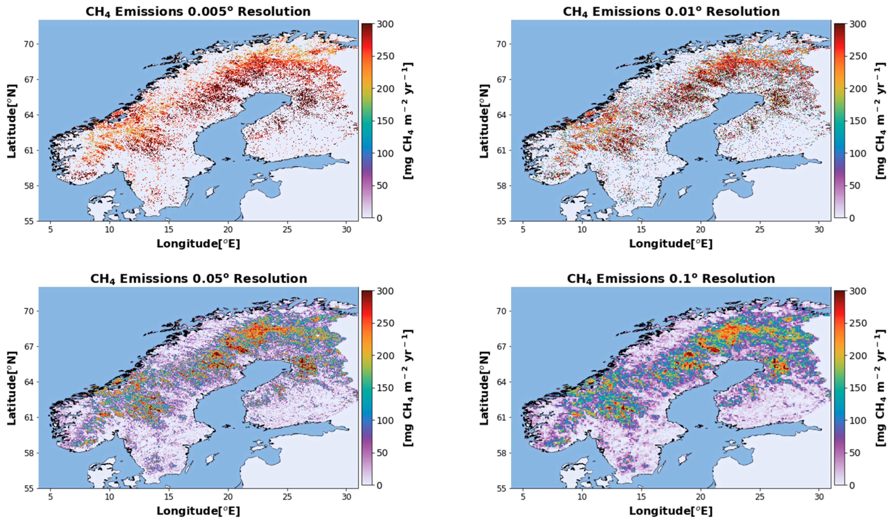
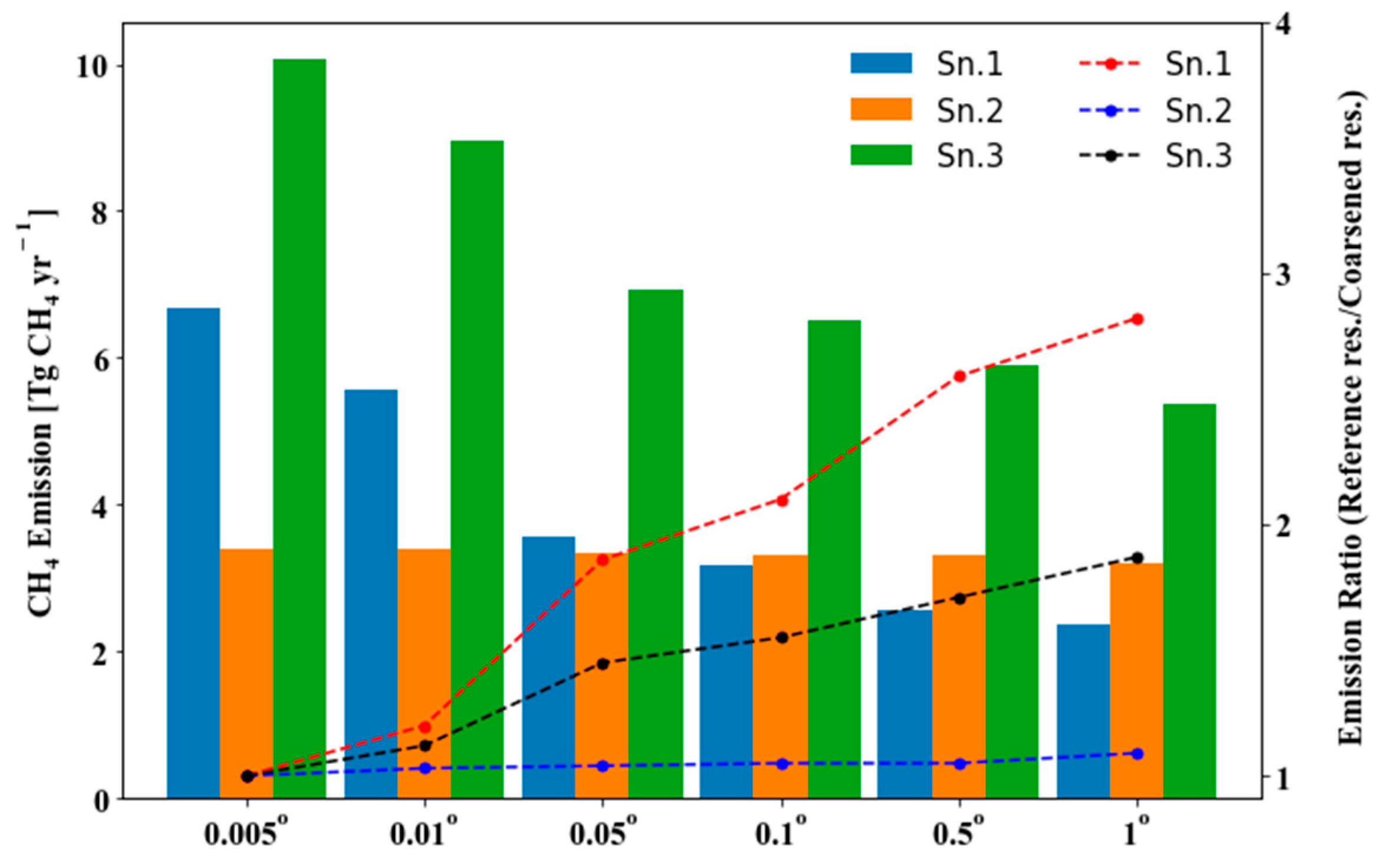
3. Results

This section presents the modeled CH₄ emissions over our Fennoscandinavian domain for the scenarios in Table 1, using the datasets described in Section 2.4, and how they vary with spatial resolution. Annual CH₄ emissions integrated over the full domain span a wide range when coarsened from the highest resolution of 0.005°, used as reference, to progressively coarser resolutions up to 1°. Note that we eliminated the coastal area effects on the resolution dependence due to coarsening of the land–sea mask; therefore, we excluded all cells nearby the shoreline such that grid boxes at the coarsest resolution are still entirely over land. This takes care in the same way for the border with Russia.

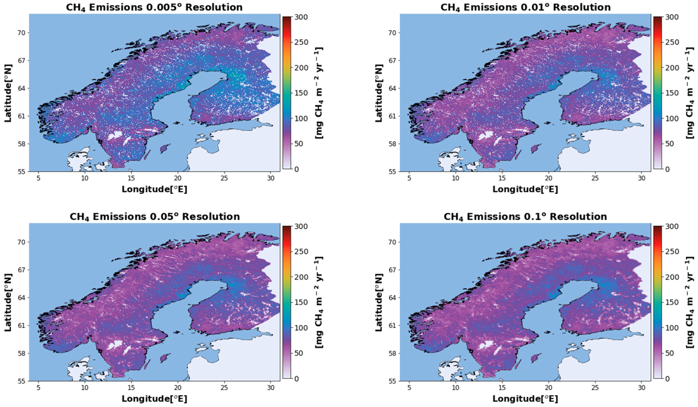
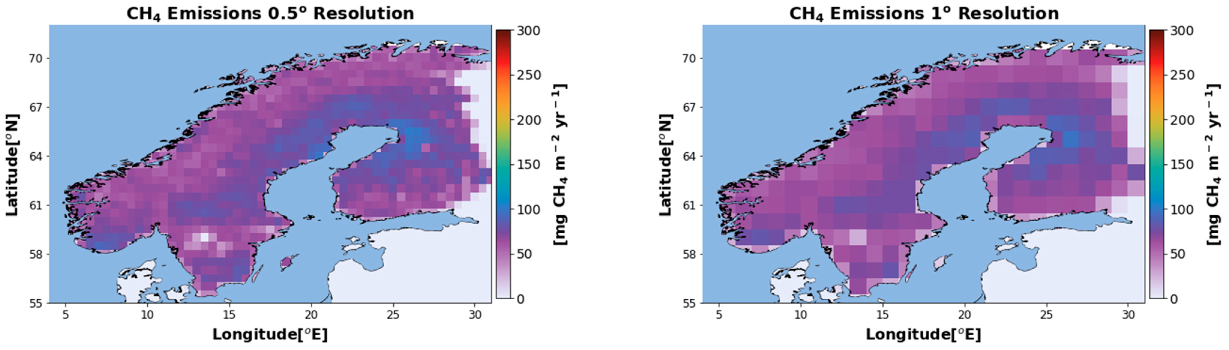
3.1. Scenario Sn.1

Figure 4 illustrates the spatial distribution of annual CH₄ emissions from wetlands across the study area. Notably, significant variations are observed across a wide range of scales, ranging from the finest resolution to the coarsest resolution of 1° × 1°. As the resolution becomes finer, the spatial pattern gradually converges. At the reference resolution, the integrated CH₄ emissions amount to approximately 6.67 Tg CH₄ yr⁻¹, surpassing the emissions at a resolution of 0.01° (~5.56 Tg CH₄ yr⁻¹) by 20%. As the resolution becomes coarser, the difference in total emissions increases. The total emissions decrease from 6.67 Tg CH₄ yr⁻¹ at the finest resolution to around 2.36 Tg CH₄ yr⁻¹ at the coarsest resolution of 1° × 1°, representing a reduction of approximately threefold compared to the emissions at the reference resolution (see

Table 3. Integrated CH₄ emissions for the study area (All scenarios).

Integrated Methane Emissions over the Study Area
Scenarios	Resolution (°)	0.005°	0.01°	0.05°	0.1°	0.5°	1°
Sn.1	Total Emissions (Tg CH4 yr−1)	6.67	5.56	3.58	3.17	2.57	2.36
	CH4 (Ref. Resolution */Resolution **)	1.00	1.30	1.86	2.10	2.59	2.82
Sn.2	Total Emissions (Tg CH4 yr−1)	3.4	3.39	3.36	3.33	3.32	3.21
	CH4 (Ref. Resolution */Resolution **)	1.00	1.03	1.04	1.05	1.05	1.09
Sn.3	Total Emissions (Tg CH4 yr−1)	10.07	8.95	6.94	6.5	5.89	5.37
	CH4 (Ref. Resolution */Resolution **)	1.00	1.12	1.45	1.55	1.71	1.87

* Ref. Resolution is the emission at the highest resolution (0.005°) ** Resolution is the emission from tested resolutions 0.01°, 0.05°, 0.1°, 0.5°, and 1°.

).

3.2. Scenario Sn.2

The resolution dependence for CH₄ emissions (uptake in reality) in uplands soils is less strong than for wetlands. Appendix A Figure A1 compares total CH₄ emission for the study area obtained using prescribed values for SOC and SM in Table 2. The emission ratio of each test resolution remains much closer to unity compared to Sn.1 (Table 3). The total emission at the uplands reference resolution (3.4 Tg CH₄ yr⁻¹) is only a factor of 1.09 higher than at the coarsest resolution of 1° × 1° (3.21 Tg CH₄ yr⁻¹). Since the study area is dominated by uplands, the impact of averaging to coarser resolution is expected to be less than for wetlands (see Appendix A Figure A1).

3.3. Scenario Sn.3

In this scenario, we merged Sn.1 and Sn.2 (which represent wetlands and uplands, respectively), in order to consider the fact that both soil organic carbon (SOC) and soil moisture (SM) exist in upland areas (Figure A2). Accounting for the availability of soil moisture and soil carbon in upland soils reduces the difference between upland and wetlands values, which is expected to reduce the resolution dependence. Note that in this scenario, the results assume that emissions are always positive in upland ecosystems, which usually is not the case. Nevertheless, the reason for including this scenario is to test the effect of assuming larger upland/peatland contrasts in SOC and SM in Sn.1 than will be the case in reality. As can be seen, the resolution effect in this scenario is less than in Sn.1 but still large.

In Figure 5, scenarios Sn.1–Sn.3 have been plotted together to show the difference in resolution dependence between them.

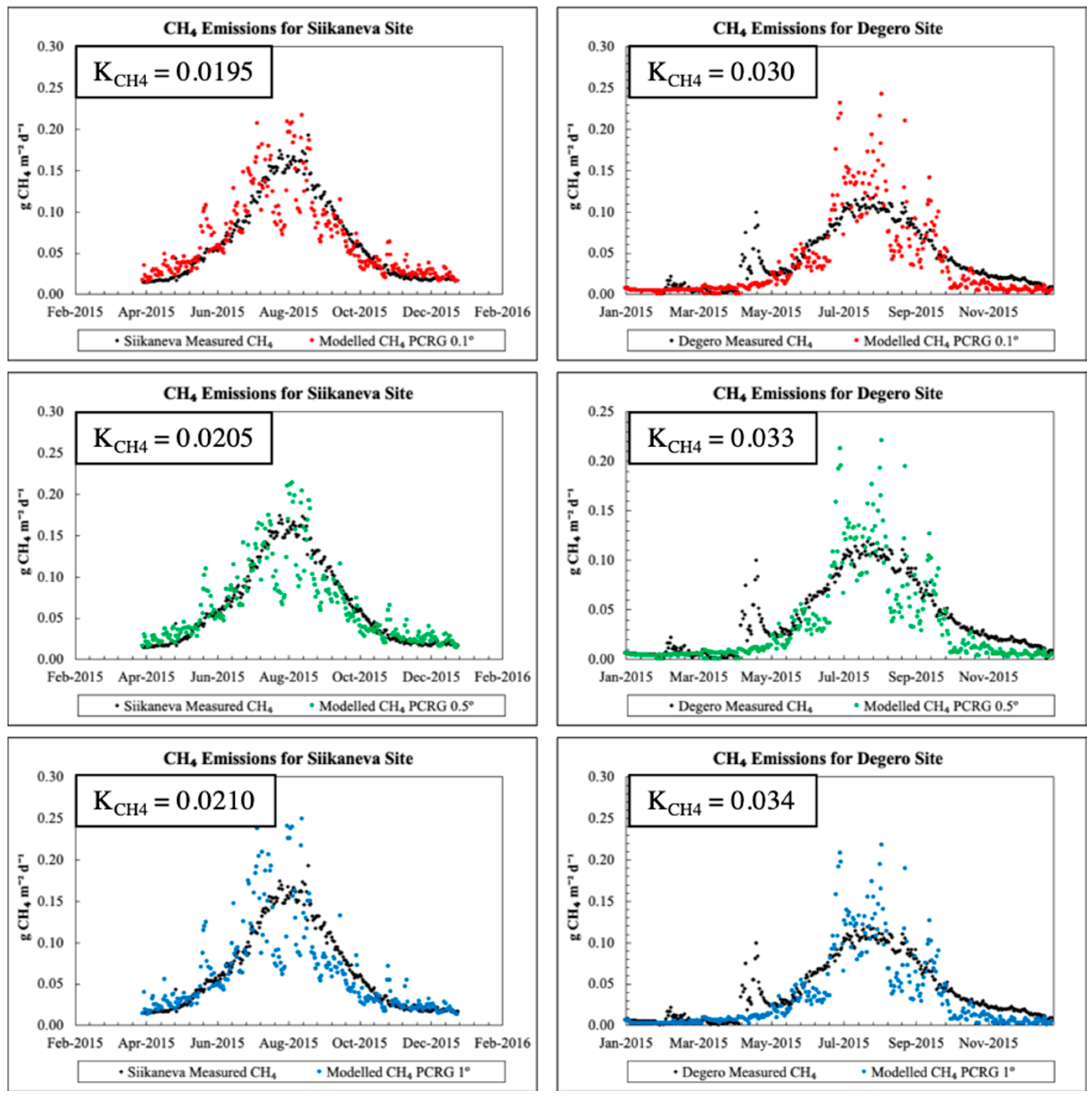
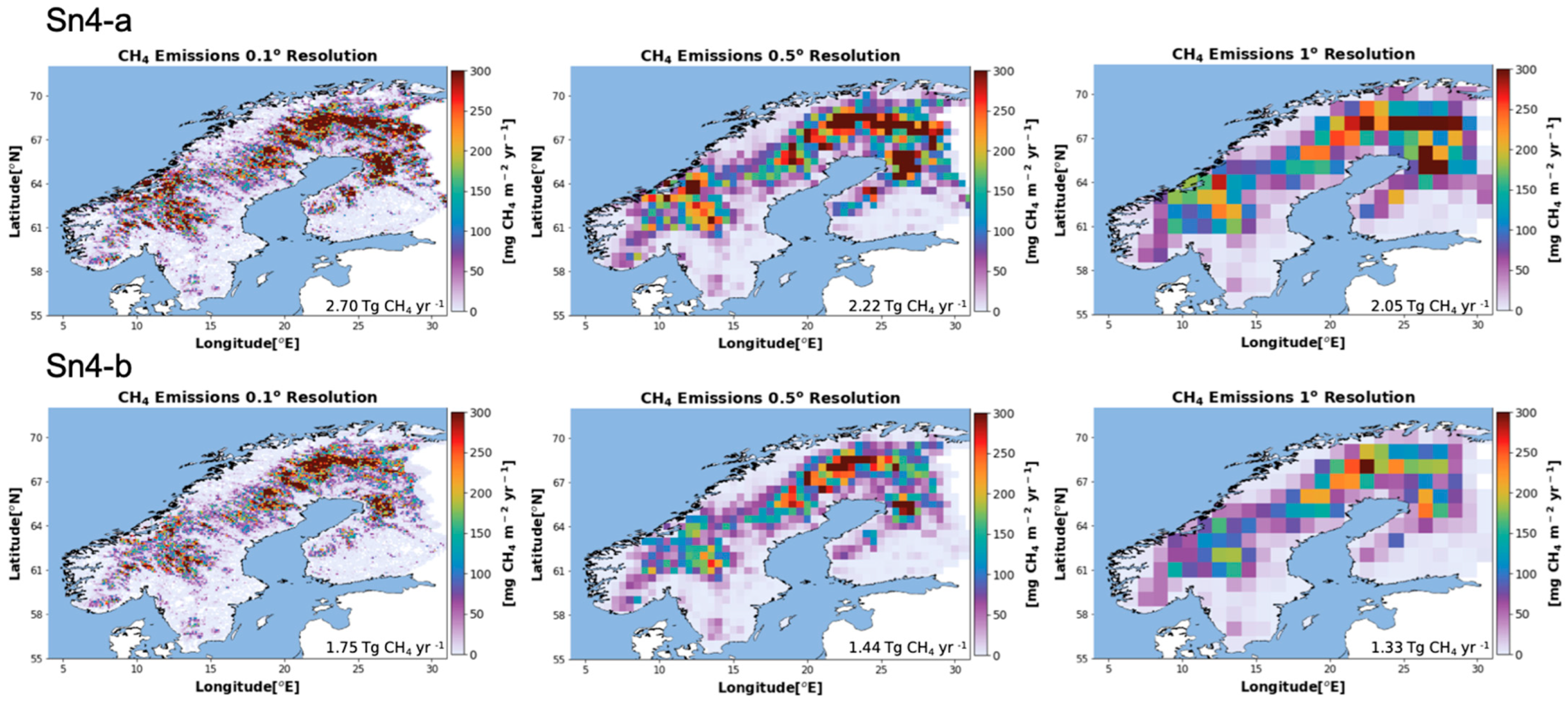
3.4. Scenario Sn.4-a and Sn.4-b

Here, the resolution dependence is computed using daily varying SM and T_soil data (see Table 1) for wetland areas only in addition to the SOC dataset. Following the same steps, we used the finest-resolution ERA5 and PCRG soil moisture data (0.1°). All participating datasets wee regridded to 0.1° (~10 × 10 km) from which coarsened maps at 0.5° (~50 × 50 km) and 1° (~100 × 100 km) were derived by aggregation.

To further improve the realism of the simulation, the emission model at 0.1° resolution was calibrated using flux measurements. As the K_CH4 values (Figure 6) are different for both Degero and Siikaneva sites at 0.1°, the K_CH4 values for both sites were averaged (K_CH4 = 0.025) and applied to Equation (5) to simulate CH₄ at 0.1°, 0.5°, and 1°.

In Sn.4-a, we applied the ERA5 soil moisture dataset to Equation (5). The results show considerable differences between the three modeled resolutions. At 0.1° resolution, we found integrated CH₄ emissions from wetlands of ~2.7 Tg yr⁻¹, which decreased by ~18% for the 0.5° to ~2.22 Tg yr⁻¹ and by ~25% for the 1° to ~2.03 Tg yr⁻¹ (Figure 7).

Sn.4-b is the same as Sn.4-a, but we swap ERA5 soil moisture with PCRG soil moisture dataset. Just like the Sn.4-a but less significant, the results show differences between the three modeled resolutions. At 0.1° resolution, we found integrated CH₄ emissions from wetlands of ~1.75 Tg yr⁻¹, which decreased by ~18% for the 0.5° to ~1.44 Tg yr⁻¹ and decreased by ~24% for the 1° to ~1.33 Tg yr⁻¹ (also see Figure 7). In a word, CH₄ emissions decreased with the increase in the resolution.

It is important to mention that we tried to calibrate the results of each resolution used in this scenario with site measurements so that each modeled resolution would agree with the measured annual total; this results in different K_CH4 values for each of the tested resolutions (Figure 6). K_CH4 values at Degero and Siikaneva decrease with the resolution, but not by much (about 10%). Using these K_CH4 values in Sn4-a, we found a domain of integrated CH₄ emissions from wetlands of ~2.7 Tg yr⁻¹ at a 0.1° resolution, which decreased by ~10% for the 0.5° to ~2.45 Tg yr⁻¹ and decreased by ~16% for the 1° to ~2.27 Tg yr⁻¹. This means that the use of different K_CH4 values partially mitigates the resolution dependence, but not enough to fully account for it. Note that this result will depend, among different factors, on the size of the wetland for which measurements are available. However, for wetlands that are smaller than the coarsest-resolution grid box, the impact is expected to be in the direction that we find for Siikaneva and Degero. This result favors the use of high-resolution models, for which the calibration will be most accurate. However, it argues against the use of high-resolution K_CH4 values in coarser resolution models.

4. Discussion

The results of our simplified wetland experiments show a strong dependence of regionally integrated CH₄ emissions on the spatial resolution that is used. The question, however, is whether this resolution dependence is representative of wetland models that are used to estimate wetland CH₄ emissions or whether it arises because of the simplicity of the setup that has been chosen. One obvious simplification is the use of grid-box-averaged soil carbon and soil moisture values. Wetland models commonly keep track of the sub-grid fraction that is covered by wetlands. In our simplified experiment, that approach fully accounts for the resolution dependence. This can readily be understood from Equation (4), indicating that the resolution dependence scales with the inverse wetland fraction (the right-hand side being 1/F_wl). Therefore, if the soil carbon and soil moisture are averaged over the wetland fraction rather than the whole grid box, then the E_HL/E_LR ratio becomes 1 and the resolution dependence vanishes.

However, a few problems remain. The first is that the wetland fraction is determined from a hydrological model or satellite data with a limited horizontal resolution, compromising the ability to determine the wetland fraction. Secondly, the representation of wetland area in models is associated with large uncertainties.

To assess the uncertainty in wetland areas, we plotted the wetlands extent maps used by the WetChimp model intercomparison [9] (

Table A1. List of wetland extent maps used for comparisons.

Model	Wetland Determination Scheme	Original Resolution (lon × lat)	Principal References
LPJ-Bern	Prescribed peatlands and monthly inundation. Simulated dynamic wet mineral soils (saturated, non-inundated).	0.5° × 0.5°	Spahni et al. [29]
LPJ-WHyMe	Prescribed peatland extents with simulated saturated/unsaturated conditions.	0.5° × 0.5°	Wania et al. [9]
LPJ-WSL	Prescribed from monthly inundation dataset.	0.5° × 0.5°	Zhen Zhang et al. [30]
ORCHIDEE	Mean yearly extent over 1993–2004 period scaled to that of inundation dataset with model calculated intra- and inter-annual dynamics.	1.0° × 1.0°	Wania et al. [9]
SDGVM	Independently simulated extents.	0.5° × 0.5°	Melton et al. [8], Singarayer et al. [9]
DLEM	Maximal extents from inundation dataset with simulated intra-annual dynamics.	0.5° × 0.5°	Melton et al. [8]
GLWD-3	Created on the basis of existing maps, data, and information, such as the Digital Chart of the World, World Conservation Monitoring Centre (WCMC) and others.	30 arc-s (0.008° × 0.008°)	Lehner et al. [31]
GIEMS	Satellite based inundated surface data for each month for 15 years (1993–2007) for each pixel on the globe.	0.25° × 0.25°	Prigent et al. [32]

) for the Fennoscandinavian Peninsula in Figure 8. For reference, the high-resolution CLC2018 wetland map is included at the same resolution of 0.5° × 0.5° to match the resolution of wetlands maps of WetChimp. Depending on the type of information that is used to determine where the wetlands are, the wetland map looks very different. Integrated over our domain, the total wetland areas represented by the models (Figure 9) are significantly different and range from 53 × 10³ to 171 × 10³ km². The Swedish Wetland Survey (VMI) reports a total wetland area of approximately 34 × 10³ km² for Sweden [26]. According to Ramsar, however, the Swedish wetland areal extent amounts only to 6655 km². If the VMI estimate from Sweden is combined with Ramsar estimates for Finland and Norway of 7795 km² and 9091 km² [27], respectively, this leads to a total wetland area for the Fennoscandinavian peninsula of 51 × 10³ km², which is in close agreement with the Corine land cover map (53 × 10³ km²).

Looking at the overall pattern of modeled wetland extent, most of the models simulate greater wetland area than CLC2018 (Figure 9). LPJ-WHyMe is in closest agreement with CLC2018 for the total wetland area (see Figure 10). However, its spatial distribution of wetlands is very different. The maps in Figure 8 and the corresponding correlation matrix in Figure 10 show large disagreements in magnitude and spatial distribution of wetland extent among the WetChimp datasets. This is primarily due to inconsistencies in (1) the definition and classification of wetland types (e.g., peatland or inundated area), (2) the time window represented by the wetland datasets, and (3) the purpose of the wetland data set and the method from which it was derived [28].

The importance of uncertainties in wetland area has been reported before [9]. The reason for mentioning it here is the implication for the correlation between wetland location and other variables, such as soil carbon and soil moisture, which are multiplied to compute CH₄ emissions as in Equation (2). It is the correlation between these terms that determines the resolution dependence. To show this, we simplify Equation (2) further so that only variations in soil moisture and soil carbon are considered. In this case, Equation (4) can be reformulated, expressing local soil moisture and soil carbon as sums of their coarse resolution mean ($\overline{SM},\overline{SOC}$) and the local deviation ($\mathsf{\Delta }\mathrm{S}M\left[i\right],\mathsf{\Delta }\mathrm{S}\mathrm{O}C\left[i\right])$. This leads to

$$\frac{E_{HR}}{E_{LR}}=1+\frac{1}{\overline{SOC.}\overline{SM.}{A}_{LR}}{\sum }_{i=0}^{i=n}\mathsf{\Delta }SOC\left[i\right] \mathsf{\Delta }SM\left[i\right]A_{HR}$$

(6)

where n is the number of high-resolution grid boxes in each low-resolution grid box. Equation (6) shows that for uncorrelated soil carbon and soil moisture, the second right-hand-side term becomes small and the ratio approaches 1. For a positive correlation, the emission increases with resolution. The effect is large if local deviations are large compared with the coarse-resolution mean. Likewise, negative correlations lead to emissions that decrease with increasing resolution. This equation explains why emission scenarios with smaller differences between upland and wetland soil carbon and soil moisture lead to smaller resolution dependences. To avoid resolution-dependent errors, it is important to obtain the correct correlation between soil carbon and soil moisture. The same is true for temperature variations, following the same logic. The challenge of obtaining the correct spatial correlation is highlighted in Figure 10, which shows the limited correlation (−0.12 on average) in wetland area between the WetChimp models over Fennyscandinavia.

Because of Equation (6), the use of wetland fractions is only sufficient to deal with resolution dependence if there is no variation between sub-grid wetland regions—the opposite is generally the case for wetlands, as their CH₄ emission is known to be highly heterogeneous. We have tried to quantify the resolution dependence that might arise from variations within the wetland fraction. The results (not shown) indicate that the impact is sizable (32% higher when aggregating from 0.1° to 0.5° and 43% higher when aggregating from 0.1° to 1°). In other words, accounting for grid cell fraction causes higher CH₄ emission estimates for wetlands when aggregating from fine to coarse resolution.

It is questionable how well the ISRIC soil organic carbon and PCRG or ERA5 soil moisture (corr. = 0.89 and 0.85 at 0.1° resolution, respectively) datasets capture the variability at their native resolutions. The role of soil carbon requires special attention because many models rather use soil respiration or vegetation productivity as a measure of the amount of available degradable carbon. However, here, no distinction is made between wetland and upland productivity, whereas in reality, the productivity in wetlands is usually much lower than in uplands due to oxygen limitation. As a result, important errors are to be expected from models failing to capture the correlation of the parameters that drive CH₄ emissions from wetlands.

A solution to mitigate resolution-dependent errors is to increase the resolution up to Eddy Covariance tower (EC) resolution, which is 100 × 100 m, in order to calibrate model results to EC measurements. As shown in this study, advanced datasets are available for achieiving this. Equally important to obtaining the correct correlation right is for these datasets to be mutually consistent. Note that this is true not only for the distinction between wetland and upland ecosystems. Large variations also occur within a single wetland.

Multivariant Probability Density Functions (PFDs) might be useful to mitigate the resolution dependence problem by determining the correlation between SM and SOC in high-resolution maps ad then applying the multi-variant PDFs of SM and SOC at the course resolution. We do not provide a solution for that but argue that an important step in the right direction can be made using high-resolution datasets that are available.

5. Conclusions

This study investigates the dependence of regionally integrated CH₄ emissions on spatial resolution. Simulations are performed for the Fennoscandinavian domain at resolutions ranging from 0.005° × 0.005° to 1° × 1°. The results of our simplified wetland experiments show that this dependence can be strong (up to 3 times greater between high and coarse resolution). In the model that is used, the effect arises from the correlation between soil moisture and soil carbon. In our experiments, the impact is effectively mitigated by accounting for the sub-grid wetland fraction. How well this works depends on how well the true wetland fraction is represented, which is a key uncertainty in wetland models. In addition, correlated variations between soil moisture and soil carbon within the wetland fraction lead to resolution-dependent errors, which are more difficult to quantify using the available datasets. The results suggest that macroscale biogeochemical models might underestimate regional CH₄ emissions due to a coarse representation of the correlation between input parameters that drive the methane emission (such as soil moisture and soil carbon). Our solution is not a straightforward recipe; however, we strongly recommend making use as much as possible of existing high-resolution datasets.

References

- Saunois, M.; Stavert, A.R.; Poulter, B.; Bousquet, P.; Canadell, J.G.; Jackson, R.B.; Raymond, P.A.; Dlugokencky, E.J.; Houweling, S. The Global Methane Budget 2000–2017. Earth Syst. Sci. Data 2020, 1561–1623. [Google Scholar] [CrossRef]
- IIPCC2013. Climate Change 2013—The Physical Science Basis; Climate Change 2013; IPCC: Geneva, Switzerland, 2013; ISBN 9781107661820. [Google Scholar]
- IPCC Climate Change 2007 Synthesis Report. Intergovernmental Panel on Climate Change; IPCC: Geneva, Switzerland, 2007. [Google Scholar]
- Anthony Bloom, A.; Bowman, W.K.; Lee, M.; Turner, J.A.; Schroeder, R.; Worden, R.J.; Weidner, R.; McDonald, C.K.; Jacob, J.D. A Global Wetland Methane Emissions and Uncertainty Dataset for Atmospheric Chemical Transport Models (WetCHARTs Version 1.0). Geosci. Model Dev. 2017, 10, 2141–2156. [Google Scholar] [CrossRef]
- Bloom, A.A.; Bowman, K.; Lee, M.; Turner, A.J.; Schroeder, R.; Worden, J.R.; Weidner, R.; McDonald, K.C.; Jacob, D.J. A Global Wetland Methane Emissions and Uncertainty Dataset for Atmospheric Chemical Transport Models. Geosci. Model Dev. Discuss. 2016, 1–37. [Google Scholar] [CrossRef]
- Silvey, C.; Jarecke, K.M.; Hopfensperger, K.; Loecke, T.D.; Burgin, A.J. Methane and Nitrous Oxide Emissions from Natural Sources. In Emissions of Methane and Nitrous Oxide from Natural Sources; Nova Science Publishers, Inc.: Hauppauge, NY, USA, 2012; pp. 1–196. ISBN 9781620816448. [Google Scholar]
- Kirschke, S.; Bousquet, P.; Ciais, P.; Saunois, M.; Canadell, J.G.; Dlugokencky, E.J.; Bergamaschi, P.; Bergmann, D.; Blake, D.R.; Bruhwiler, L.; et al. Three Decades of Global Methane Sources and Sinks. Nat. Geosci. 2013, 6, 813–823. [Google Scholar] [CrossRef]
- Melton, J.R.; Wania, R.; Hodson, E.L.; Poulter, B.; Ringeval, B.; Spahni, R.; Bohn, T.; Avis, C.A.; Beerling, D.J.; Chen, G.; et al. Present State of Global Wetland Extent and Wetland Methane Modelling: Conclusions from a Model Inter-Comparison Project (WETCHIMP). Biogeosciences 2013, 10, 753–788. [Google Scholar] [CrossRef]
- Wania, R.; Melton, J.R.; Hodson, E.L.; Poulter, B.; Ringeval, B.; Spahni, R.; Bohn, T.; Avis, C.A.; Chen, G.; Eliseev, A.V.; et al. Present State of Global Wetland Extent and Wetland Methane Modelling: Methodology of a Model Inter-Comparison Project (WETCHIMP). Geosci. Model Dev. 2013, 6, 617–641. [Google Scholar] [CrossRef]
- Matthews, E.; Fung, I. Methane Emission from Natural Wetlands: Global Distribution, Area, and Environmental Characteristics of Sources. Global Biogeochem. Cycles 1987, 1, 61–86. [Google Scholar] [CrossRef]
- Zhang, Z.; Zimmermann, N.E.; Stenke, A.; Li, X.; Hodson, E.L.; Zhu, G.; Huang, C.; Poulter, B. Emerging Role of Wetland Methane Emissions in Driving 21st Century Climate Change. Proc. Natl. Acad. Sci. USA 2017, 114, 9647–9652. [Google Scholar] [CrossRef]
- Peltola, O.; Vesala, T.; Gao, Y.; Räty, O.; Alekseychik, P.; Aurela, M.; Chojnicki, B.; Desai, A.R.; Dolman, A.J.; Euskirchen, E.S.; et al. Monthly Gridded Data Product of Northern Wetland Methane Emissions Based on Upscaling Eddy Covariance Observations. Earth Syst. Sci. Data Discuss. 2019, 11, 1263–1289. [Google Scholar] [CrossRef]
- Zheng, B.; Zhang, Q.; Tong, D.; Chen, C.; Hong, C.; Li, M.; Geng, G.; Lei, Y.; Huo, H.; He, K. Resolution Dependence of Uncertainties in Gridded Emission Inventories: A Case Study in Hebei, China. Atmos. Chem. Phys. 2017, 17, 921–933. [Google Scholar] [CrossRef]
- Zhu, X.; Zhuang, Q.; Lu, X.; Song, L. Spatial Scale-Dependent Land-Atmospheric Methane Exchanges in the Northern High Latitudes from 1993 to 2004. Biogeosciences 2014, 11, 1693–1704. [Google Scholar] [CrossRef]
- Awuah, K.T. Effects of Spatial Resolution, Land-Cover Heterogeneity and Different Classification Methods on Accuracy of Land-Cover Mapping; Southern Swedish Forest Research Centre: Alnarp, Sweden, 2017. [Google Scholar] [CrossRef]
- Gedney, N.; Cox, P.M.; Huntingford, C. Climate Feedback from Wetland Methane Emissions. Geophys. Res. Lett. 2004, 31, 1–4. [Google Scholar] [CrossRef]
- Büttner, G.; Kostztra, B.; Soukup, T.; Sousa, A.; Langanke, T. CLC2018 Technical Guidelines; European Environment Agency: Copenhagen, Denmark, 2017; 60p.
- Faltan, V.; Petrovič, F.; Ot’ahel’, J.; Feranec, J.; Druga, M.; Hruška, M.; Nováček, J.; Solár, V.; Mechurová, V. Comparison of CORINE Land Cover Data with National Statistics and the Possibility to Record This Data on a Local Scale-Case Studies from Slovakia. Remote Sens. 2020, 12, 2484. [Google Scholar] [CrossRef]
- Kosztra, B.; Büttner, G.; Hazeu, G.; Arnold, S. Updated CLC Illustrated Nomenclature Guidelines; European Environment Agency: Copenhagen, Denmark, 2017; pp. 1–124.
- Hengl, T.; De Jesus, J.M.; Heuvelink, G.B.M.M.; Gonzalez, M.R.; Kilibarda, M.; Blagotić, A.; Shangguan, W.; Wright, M.N.; Geng, X.; Bauer-Marschallinger, B.; et al. SoilGrids250m: Global Gridded Soil Information Based on Machine Learning. PLoS ONE 2017, 12, e0169748. [Google Scholar] [CrossRef] [PubMed]
- Schaufler, G.; Kitzler, B.; Schindlbacher, A.; Skiba, U.; Sutton, M.A.; Zechmeister-Boltenstern, S. Greenhouse Gas Emissions from European Soils under Different Land Use: Effects of Soil Moisture and Temperature. Eur. J. Soil Sci. 2010, 61, 683–696. [Google Scholar] [CrossRef]
- Muñoz Sabater, J. ERA5-Land Monthly Averaged Data from 1981 to Present; Copernicus Climate Change Service (C3S), Climate Data Store (CDS): Brno, Czech Republic, 2019. [Google Scholar] [CrossRef]
- Sutanudjaja, E.H.; van Beek, L.P.H.; Drost, N.; de Graaf, I.E.M.; de Jong, K.; Peßenteiner, S.; Straatsma, M.W.; Wada, Y.; Wanders, N.; Wisser, D.; et al. PCR-GLOBWB 2.0: A 5 Arc-Minute Global Hydrological and Water Resources Model. Geosci. Model Dev. 2018, 11, 2429–2453. [Google Scholar] [CrossRef]
- Walter, B.P.; Heimann, M. A Process-Based, Climate-Sensitive Model to Derive Methane Emissions from Natural Wetlands: Application to Five Wetland Sites, Sensitivity to Model Parameters, and Climate. Global Biogeochem. Cycles 2000, 14, 745–765. [Google Scholar] [CrossRef]
- Ringeval, B.; De Noblet-Ducoudré, N.; Ciais, P.; Bousquet, P.; Prigent, C.; Papa, F.; Rossow, W.B. An Attempt to Quantify the Impact of Changes in Wetland Extent on Methane Emissions on the Seasonal and Interannual Time Scales. Global Biogeochem. Cycles 2010, 24, 1–12. [Google Scholar] [CrossRef]
- Gunnarsson, U.; Löfroth, M. The Swedish Wetland Survey—Compiled Excerpts From The National Final Report; Swedish Environmental Protection Agency: Stockholm, Sweeden, 2014; ISBN 9789162066185.
- Party, E.C.; Importance, I. The List of Wetlands of International Importance. Available online: https://www.ramsar.org/sites/default/files/documents/library/sitelist.pdf (accessed on 9 May 2023).
- Zhang, B.; Tian, H.; Lu, C.; Chen, G.; Pan, S.; Anderson, C.; Poulter, B. Methane Emissions from Global Wetlands: An Assessment of the Uncertainty Associated with Various Wetland Extent Data Sets. Atmos. Environ. 2017, 165, 310–321. [Google Scholar] [CrossRef]
- Spahni, R.; Wania, R.; Neef, L.; Van Weele, M.; Pison, I.; Bousquet, P.; Frankenberg, C.; Foster, P.N.; Joos, F.; Prentice, I.C.; et al. Constraining Global Methane Emissions and Uptake by Ecosystems. Biogeosciences 2011, 8, 1643–1665. [Google Scholar] [CrossRef]
- Zhang, Z.; Zimmermann, N.E.; Kaplan, J.O.; Poulter, B. Modeling Spatiotemporal Dynamics of Global Wetlands: Comprehensive Evaluation of a New Sub-Grid TOPMODEL Parameterization and Uncertainties. Biogeosciences 2016, 13, 1387–1408. [Google Scholar] [CrossRef]
- Lehner, B.; Döll, P. Development and Validation of a Global Database of Lakes, Reservoirs and Wetlands. J. Hydrol. 2004, 296, 1–22. [Google Scholar] [CrossRef]
- Prigent, C.; Jimenez, C.; Bousquet, P. Satellite-Derived Global Surface Water Extent and Dynamics Over the Last 25 Years (GIEMS-2). J. Geophys. Res. Atmos. 2020, 125, e2019JD030711. [Google Scholar] [CrossRef]