Abstract
The prediction of sea level rise is extremely important for improved future climate change mitigation and adaptation strategies. This study uses a hybrid convolutional neural Network (CNN) and a bidirectional long short-term (BiLSTM) model with successive variational mode decomposition (SVMD) to predict the absolute sea level for two study sites in Australia (Port Kembla and Milner Bay). More importantly, the sea level measurements using a tide gauge were corrected using Global Navigation Satellite System (GNSS) measurements of the vertical land movement (VLM). The SVMD-CNN-BiLSTM model was benchmarked by a multi-layer perceptron (MLP), support vector regression (SVR) and gradient boosting (GB). The SVMD-CNN-BiLSTM model outperformed all the comparative models with high correlation values of more than 0.95 for Port Kembla and Milner Bay. Similarly, the SVMD-CNN-BiLSTM model achieved the highest values for the Willmott index, the Nash–Sutcliffe index and the Legates and McCabe index for both study sites. The projected linear trend showed the expected annual mean sea rise for 2030. Using the current trend, Port Kembla was projected to have an MSL value of 1.03 m with a rate rise of approx. 4.5 mm/year. The rate of the MSL for Milner Bay was comparatively lower with a value of approx. 2.75 mm/year and an expected MSL value of 1.27 m for the year 2030.
1. Introduction
The anticipated rise in sea level caused by climate change has many potential consequences, including flooding, shoreline retreat, ecosystem imbalance and the invasion of salt water into freshwater systems. This endangers 60% of the world’s population that lives in coastal areas [1]. The situation is particularly acute for communities on small islands which may become uninhabitable [2,3]. These impacts motivate using long-term sea level rise modeling as a tool to understand the trends and accurately predict sea level rise in the future. However, the accuracy and reliability of these predictions should consider certain important aspects, such as the absolute sea level rise, which accounts for land subsidence. In this paper, we model the vertical land motion (VLM) [4]-corrected absolute sea level at two separate geographical locations in Australia using a novel deep learning artificial intelligence model based on successive variational mode decomposition (SVMD) [5], a convolutional neural network (CNN) [6] and bidirectional long short-term memory (BiLSTM) [7]. The VLM consideration is extremely important because the position of the sea floor changes over time, and therefore the measured sea level should be corrected for this variability for accurate estimation [4]. The VLM has many root causes, including tides, plate tectonic movements, earthquakes, glacial activity and human actions. While the typical values are significantly less than 10 mm year−1, they can be as large as 100 mm year−1 in some extreme cases [8]. Given that the order of magnitude of typical VLM values is the same as the changes to the mean sea level, these values cannot be ignored and sea level measurements must be corrected.
LSTM models are well known to be reliable for modeling time series data such as the mean sea level. They are a type of recurrent neural network (RNN) in that they use feedback connections. However, unlike plain RNNs, they do not suffer from vanishing gradients during training, which affects the convergence of the model fit [9]. LSTM models are generally considered to be superior to traditional approaches, such as autoregressive integrated moving average (ARIMA) models [10] and bidirectional LSTM models (i.e., a BiLSTM), in which training data is fed in both directions through the model [11]. Previous research studies into sea level modeling have used different techniques. For example, in [12], the authors employed a simple linear regression with independent variables, including wind speed and pressure, to predict sea level rise. The model, while coarse, was able to explain 74% of the total observed subtidal frequency sea level in Atlantic City, New Jersey. The study in [13] compared chaos theory and ARIMA models for daily, weekly, 10-day and monthly sea levels at the Cocos Islands from 1992 to 2001 and found that the chaos theory models were slightly superior. Other studies have also used various AI models, such as artificial neural networks (ANNs), to model sea level. A study modeling the surface water levels in the Caspian Sea identified a similar accuracy between an ARIMA model and a basic 3-layer ANN model (comprising input, hidden and output layers) [14]. The study in [15] compared ARIMA, support vector regression (SVR) and LSTM models for sea levels, with the LSTM model exhibiting a significantly higher accuracy. Various other studies used different types of ANNs and deep learning to model sea level. However, no other study considered the VLM correction for absolute sea level, the SVMD data decomposition or a hybrid model. Hence, this study presents a new deep learning hybrid CNN-BiLSM model to predict the absolute sea level after GNSS-VLM for Australian sites with a data decomposition of the wave signals.
2. Materials and Methods
2.1. Study Area and Dataset
Two study sites situated in Australia were selected for this study. The two sites were located on different sides of Australia and provided a good comparison for absolute sea level rise. Table 1 and Figure 1 describe the location and geographical details. The datasets were extracted from the Australian Meteorological website (Australian Baseline Sea Level Monitoring Project (bom.gov.au) accessed on 15 May 2022).

Table 1.
The geographical details of the study site locations in Australia.
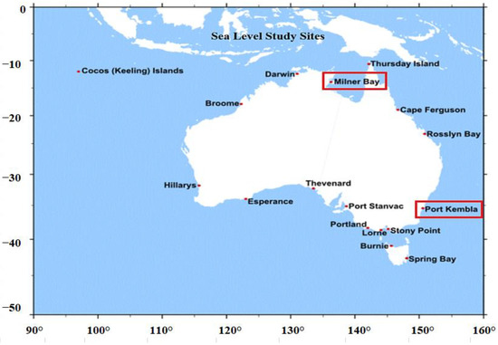
Figure 1.
The map of Australia showing the locations of the two study sites. The red rectangle shows the two study sites.
2.2. Data Preprocessing
The datasets were corrected for missing values, which were indicated with ‘−9999’. This was processed in Python using the dataframe.interpolate function. The Australian Meteorological website (Australian Baseline Sea Level Monitoring Project (bom.gov.au) accessed on 15 May 2022) maintains high quality data and the relative proportion of missing or bad values in each file is small. After the correction of the missing values, the dataset was checked for stationarity. This is an important step in time series data analysis [16]. The following result showed the analysis of stationarity for the Milner Bay dataset using the augmented Dickey–Fuller (ADF) test [17,18]. The test statistic should be less than the critical values at 1%, 5% and 10% for the null hypothesis to be rejected. Based on the test statistic, a conclusion was made that the dataset was stationary. Table 2 shows that the test statistic was less than the critical values for the stationarity test. The dataset was then subjected to autocorrelation and partial autocorrelation analyses to determine the correlation lags, as shown in Figure 2. All the input parameters were checked for correlation with the mean sea level and computed as a matrix, as given in Figure 3. The dataset was normalized using Equation (1) and then denormalized using Equation (2) after modeling.
Table 2.
The augmented Dickey–Fuller (ADF) test results for Milner Bay.
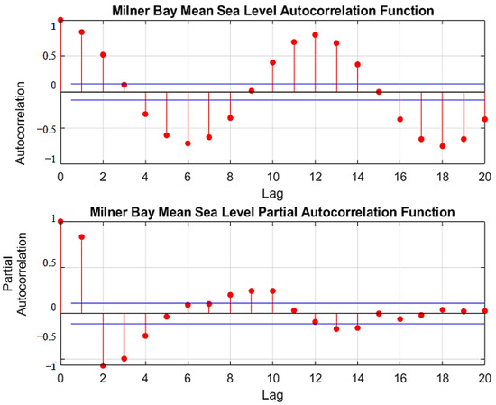
Figure 2.
The ACF and PCF for Milner Bay. The blue line shows the boundary of lag significance and red dots show the Partial Autocorrelation lags.
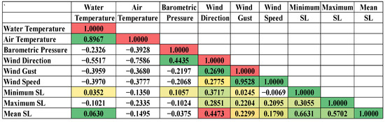
Figure 3.
The correlation matrix for the Port Kembla mean sea level with each input feature (SL—Sea Level). The darker green shades show a high correlation and the orange to red shades show a weaker correlation among the sea level parameters.
2.3. GNSS-VLM Correction of Port Kembla and Milner Bay
The Global Positioning System (GPS) is part of the Global Navigation Satellite System (GNSS) which allows for accurate measurements of the Earth’s surface [19]. It is used to locate the position of a receiver using a constellation of numerous artificial satellites [20,21]. This study uses the GNSS-VLM dataset in [22] derived from continuously operating GPS stations operated by the Nevada Geodetic Laboratory. Table 3 shows the information for Port Kembla and Milner Bay.
Table 3.
The GNSS-VLM details for Port Kembla and Milner Bay.
2.4. Signal Decomposition by Successive Variational Mode Decomposition (SVMD)
SVMD is an efficient signal decomposition technique which extracts underlying modes of the input signal into its intrinsic mode functions (IMFs) [23]. It has a lower computational complexity compared to VMD and is less sensitive to the initial values of the central frequencies of the modes [5]. These modes are orthogonal and are separated by the respective bands. The highest frequency is removed from the original signal iteratively until the residual is left as a monotonic function [24]. The process of signal decomposition is very important in data modeling as it helps to extract important features and improves the training model efficiency [25]. The Hs wave signal for both study sites were fed through the SVMD algorithm. The algorithm parameters of the compactness mode, step of dual ascend, tolerance of convergence, stopping criteria and sampling frequency were determined through trial runs before extracting the decomposed intrinsic modes. Figure 4 shows the Milner Bay signal decomposed into its IMFs using the SVMD technique for this study.
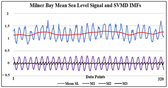
Figure 4.
The data decomposition into its IMFs using the SVMD algorithm.
2.5. Data Partition
Data partitioning is an essential step in data modeling that ensures the optimum data for each sample in training, validation and testing [26]. Table 4 shows the 60% training, 20% validation and 20% testing dataset breakdown used in this study.
Table 4.
The data partition for the period 1995–2021 into training, validation and testing.
2.6. Objective Model and Modeling Process
The objective model selected for this study was the hybrid deep learning model CNN-BiLSTM. The CNN-BiLSTM model can utilize the benefits of the CNN algorithm and two layers of the LSTM model to process the data inputs effectively for data training and forecasting. A CNN is a deep learning convolutional neural network consisting of multiple layers of artificial neurons [27]. This study used a one-dimensional convolutional layer which added a filter to the model architecture for convolution. This process of one-dimensional convolution helped to extract valuable information from the data inputs. The next stage of data processing was then conducted using the BiLSTM layers. The BiLSTM layers were widely used in time series analysis due to their ability to expand according to the sequence of time [28]. The BiLSTM platform in the study consisted of two LSTM layers (a forward and a reverse LSTM layer). Each BiLSTM layer had two LSTM networks, which processed the input dataset. A LSTM model is a network designed to overcome gradient explosion and gradient disappearance in a RNN [28,29]. The hybrid CNN-BiLSTM model had the additional capability of utilizing the CNN feature extraction superior ability and the BiLSTM architecture, which further processed these using the forward and backward neural layers. This approach of using the hybrid deep learning model performed better than the standalone models in multiple past studies [30,31,32].
Table 5 shows the model parameters, which were obtained using Grid-Search optimization for optimum results. Figure 5 illustrates the data analysis in Python and how the layers were arranged within the hybrid deep learning model architecture. Figure 6 shows the overall modeling process.
Table 5.
The CNN-BiLSTM model parameters.
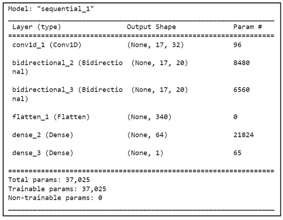
Figure 5.
The CNN-BiLSTM modeling architecture.
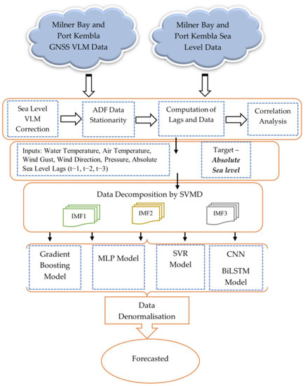
Figure 6.
Schematic diagram of the data modeling process to forecast sea level.
2.7. Benchmark Models
2.7.1. Multi-Layer Perceptron
A multi-layer perceptron (MLP) is a supervised learning algorithm that learns on a nonlinear function by utilizing backpropagation [33]. It usually conists of at least three layers of nodes, i.e., an input layer, a hidden layer and an output layer. Apart from the input layer, each node consists of a nonlinear activation function. The data transfer is only conducted in a forward direction [34].
2.7.2. Gradient Boosting
Gradient boosting (GB) utilizes a set of weak learners that perform slightly better than random guessing to develop a single strong learner [35,36]. The regularization of the hyperparameters helps to control the additive process of gradient boosting. Shrinking is applied to reduce each gradient descent step to naturally achieve regularization [37].
2.7.3. Support Vector Regression
Rooted in the Vapnik-Chervonenkis (VC) theory, support vector regression (SVR) is characterized by the use of kernels, a sparse solution, a control of margin and support vectors [38]. It is a supervised learning approach where the dataset is trained using a symmetrical loss function, which equally penalizes high and low misestimates.
2.8. Performance Evaluation Metrics
Eight evaluation metrics were used for this study for the model performance comparison. Every metric shown below (Equations (3)–(9)) added an important aspect of performance evaluation and justified the accuracy of the model performance in sea level prediction for the study sites.
- Correlation Coefficient (r)
- Willmott’s Index of Agreement (d)
- Nash–Sutcliffe Coefficient (NS)
- Legates and McCabe Index (LM)
- Root Mean Square Error (RMSE)
- Mean Absolute Error (MAE)
- Relative Root Mean Square Error (RRMSE)
- Mean Absolute Percentage Error (MAPE)where is the simulated data and is the observed data.
3. Results and Discussion
The prediction results from the testing phase were compared with the observational dataset by computing the performance and error metrics. Table 6, Table 7, Table 8 and Table 9 show the performance metrics for the objective model (SVMD-CNN-BiLSTM) and the three benchmark models (SVMD-MLP, SVMD-SVR, SBMD-GB).
Table 6.
Model performance metrics for Port Kembla.
Table 7.
Model error metrics for Port Kembla.
Table 8.
Model performance metrics for Milner Bay.
Table 9.
Model error metrics for Milner Bay.
This study developed a hybrid SVMD-CNN-BiLSTM deep learning model for VLM-corrected mean sea level prediction. Other well-known AI models were also used for the prediction of the VLM-corrected sea level. Hence, to analyze and compare the efficiency of these models, all the model results were used to calculate the performance and error metrics to evaluate the prediction ability. Figure 7 and Figure 8 illustrate scatterplots which display the strength of the association between the observed and predicted values. Figure 9 and Figure 10 show the time series comparison for the model prediction with the observed values for both study sites. The SVMD-CNN-BiLSTM model showed a strong association and the best results for both study sites.
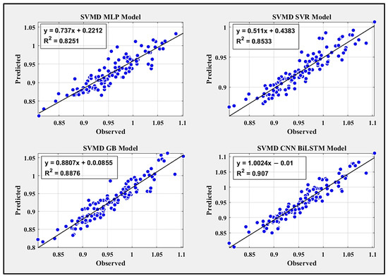
Figure 7.
Scatterplot for Port Kembla showing the correlation between the observed and the predicted values.
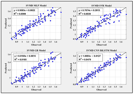
Figure 8.
Scatterplot for Milner Bay showing the correlation between the observed and the predicted values.
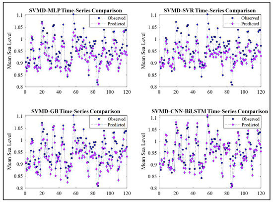
Figure 9.
Time series comparison for Port Kembla showing the mean sea level tracking accuracy for each model.
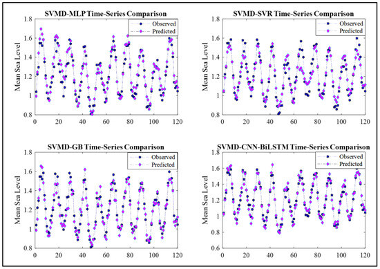
Figure 10.
Time series comparison for Milner Bay showing the mean sea level tracking accuracy for each model.
Figure 11 and Figure 12 show the model performance of the two study sites based on the computation of the correlation coefficient, Willmott’s index, the Nash–Sutcliffe coefficient and the Legates and McCabe index. The correlation coefficient was an important statistical measure and showed the degree of association between the observed and predicted VLM-corrected mean sea level [39]. Willmott’s index of agreement was a measure of the variability between the observed and predicted data and is commonly used in climate modeling [40]. Nash–Sutcliffe index is mostly used in water quality models and provided a goodness of fit for the evaluated models [41]. The Legates and McCabe index is a variant of the Nash–Sutcliffe index and is considered a more refined index of the model performance, which compared the agreement between the observed and predicted data [42]. All the models showed a high correlation with values of greater than 0.9 for both study sites. The SVMD-CNN-BiLSTM model attained the highest value at both study sites with values of 0.9524 and 0.9736 for Port Kembla and Milner Bay, respectively. Similarly, the SVMD-CNN-BiLSTM model achieved the highest values for Willmott’s index (0.9457), the Nash–Sutcliffe index (0.8790) and the Legates and McCabe index (0.6581) for Port Kembla. Milner Bay also showed superior results for the SVMD-CNN-BiLSTM model with Willmott’s Index (0.9717), the Nash–Sutcliffe index (0.9439) and the Legates and McCabe index (0.7781).
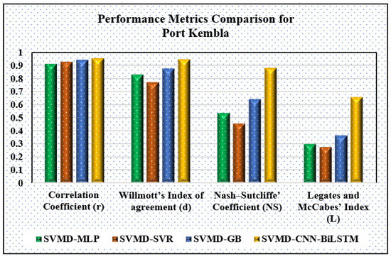
Figure 11.
Performance metrics for Port Kembla.
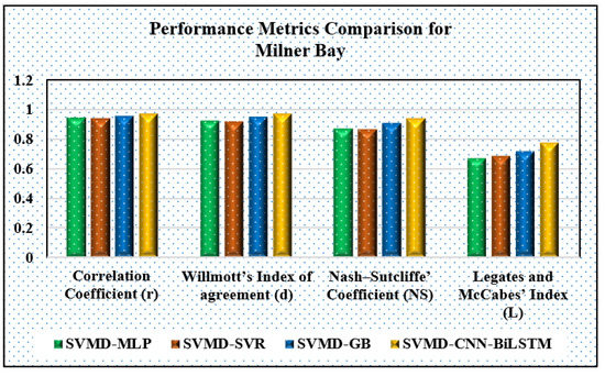
Figure 12.
Performance metrics for Milner Bay.
The computation of more than one error metric for evaluation was as important as the performance metrics to ensure a comprehensive evaluation [43]. The error results also supported the superior performance of the objective model with lower values of the RMSE (0.02), MABE (0.016), RRMSE (2.096) and MAPE (1.6740) for Port Kembla and the RMSE (0.051), MABE (0.041), RRMSE (4.184) and MAPE (3.403) for Milner Bay. Figure 13 and Figure 14 show the graphic comparison of these results.
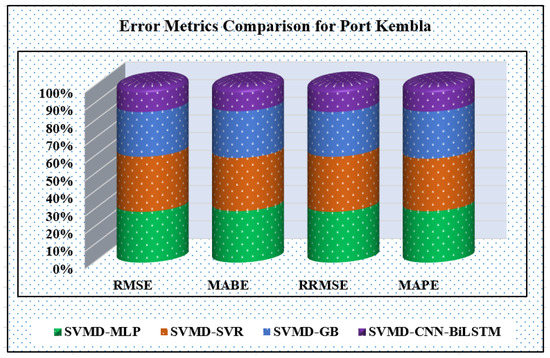
Figure 13.
Error metrics for Port Kembla.
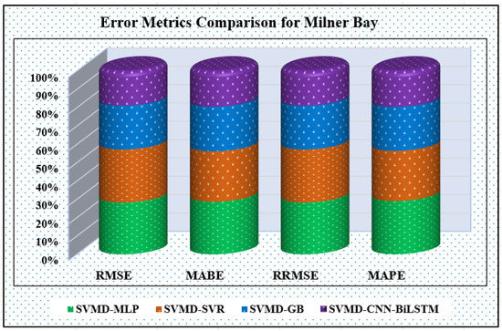
Figure 14.
Error metrics for Milner Bay.
Figure 15 and Figure 16 provide the VLM-corrected mean sea level trend analysis for Port Kembla and Milner Bay. The GNSS-VLM correction was made for the MSL annual values for the trend analysis using three period moving averages and the SVMD-CNN-BiLSTM model tracking. The projected linear trend showed the expected rise for 2030. The annual mean MSL was closely tracked by the developed objective model, which confirmed its high accuracy and its ability to predict the MSL values. Using the current trend, Port Kembla would have a MSL value of 1.03 m with a rate rise of about 4.5 mm/year, which was slightly lower than the values of 6.5 mm/year in [44]. This was due to the consideration of land subsidence and future projected values based on past trends. The rate of the MSL for Milner Bay was comparatively lower, with a value of about 2.75 mm/year and an expected MSL value of 1.27 m for the year 2030.
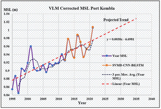
Figure 15.
VLM-corrected mean sea level trend prediction for Port Kembla using the moving average and SVMD-CNN-BiLSTM model tracking.
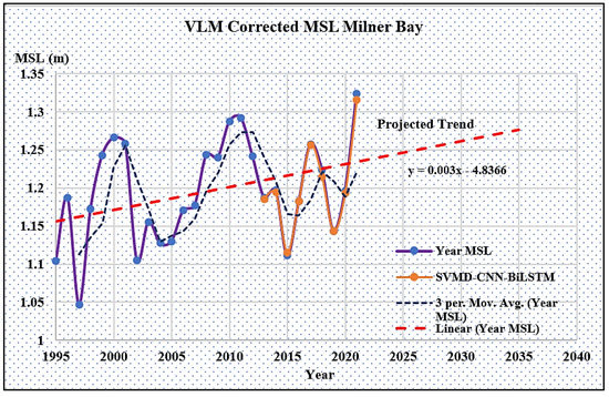
Figure 16.
VLM-corrected mean sea level trend prediction for Milner Bay using the moving average and SVMD-CNN-BiLSTM model tracking.
4. Conclusions
In this study, we developed a hybrid SVMD-CNN-BiLSTM deep learning model for VLM-corrected mean sea level prediction at two sites in Australia, namely Port Kembla and Milner Bay. This model outperformed the three other benchmark models (SVMD-MLP, SVMD-SVR and SBMD-GB) in terms of their metrics, such as the correlation coefficient, Willmott’s index, the Nash–Sutcliffe coefficient and the Legates and McCabe index, thus supporting its superior performance. The study also confirmed the importance of using a data decomposition method to extract important features from wave signals. The prediction of the absolute mean sea level accurately assists with careful planning and decision making for the future. The study successfully provided an insight into the trend by allowing for the linear projection of the sea level rise. Using the current trend, Port Kembla will have an MSL rise of approx. 4.5 mm/year and 1.27 m for Milner Bay will reach a 1.27 m rise by the year 2030. This study can be extended to other areas for accurate predictions of the MSL.
Author Contributions
Conceptualization, N.R.; methodology, N.R.; software, N.R.; validation, N.R.; formal analysis, N.R.; investigation, N.R.; resources, N.R.; data curation, N.R; writing—original draft preparation, N.R; writing—review and editing, N.R. and J.B.; visualization, N.R.; supervision, N.R; project administration, N.R; funding acquisition, N/A. All authors have read and agreed to the published version of the manuscript.
Funding
This research received no external funding.
Data Availability Statement
Not applicable.
Conflicts of Interest
The author declares no conflict of interest.
References
- Hinrichsen, D. Coastal Waters of the World: Trends, Threats, and Strategies; Island Press: Washington, DC, USA, 1998. [Google Scholar]
- Janif, S.Z.; Nunn, P.D.; Geraghty, P.; Aalbersberg, W.; Thomas, F.R.; Camailakeba, M. Value of traditional oral narratives in building climate-change resilience: Insights from rural communities in Fiji. Ecol. Soc. 2016, 21, 2. [Google Scholar] [CrossRef]
- Bijlsma, L.; Ehler, C.N.; Klein, R.J.T.; Kulshrestha, S.M.; McLean, R.F.; Mimura, N.; Nicholls, R.J.; Nurse, L.A.; Nieto, H.P.; Stakhiv, E.Z.; et al. Coastal Zones and Small Islands; Cambridge University Press: Cambridge, UK; New York, NY, USA, 1996; pp. 289–324. [Google Scholar]
- Santamaría-Gómez, A.; Gravelle, M.; Dangendorf, S.; Marcos, M.; Spada, G.; Wöppelmann, G. Uncertainty of the 20th century sea-level rise due to vertical land motion errors. Earth Planet. Sci. Lett. 2017, 473, 24–32. [Google Scholar] [CrossRef]
- Nazari, M.; Sakhaei, S.M. Successive variational mode decomposition. Signal Process. 2020, 174, 107610. [Google Scholar] [CrossRef]
- Gu, J.; Wang, Z.; Kuen, J.; Ma, L.; Shahroudy, A.; Shuai, B.; Liu, T.; Wang, X.; Wang, G.; Cai, J.; et al. Recent advances in convolutional neural networks. Pattern Recognit. 2018, 77, 354–377. [Google Scholar] [CrossRef]
- Raj, N.; Brown, J. An EEMD-BiLSTM Algorithm Integrated with Boruta Random Forest Optimiser for Significant Wave Height Forecasting along Coastal Areas of Queensland, Australia. Remote Sens. 2021, 13, 1456. [Google Scholar] [CrossRef]
- Oelsmann, J.; Passaro, M.; Dettmering, D.; Schwatke, C.; Sánchez, L.; Seitz, F. The zone of influence: Matching sea level variability from coastal altimetry and tide gauges for vertical land motion estimation. Ocean. Sci. 2021, 17, 35–57. [Google Scholar] [CrossRef]
- Hu, Y.; Huber, A.; Anumula, J.; Liu, S.-C. Overcoming the vanishing gradient problem in plain recurrent networks. arXiv 2018, arXiv:1801.06105 2018. [Google Scholar]
- Nelson, B.K. Time series analysis using autoregressive integrated moving average (ARIMA) models. Acad. Emerg. Med. 1998, 5, 739–744. [Google Scholar] [CrossRef]
- Siami-Namini, S.; Tavakoli, N.; Namin, A.S. The performance of LSTM and BiLSTM in forecasting time series. In Proceedings of the 2019 IEEE International Conference on Big Data (Big Data), Los Angeles, CA, USA, 9–12 December 2019; IEEE: Piscataway, NJ, USA, 2019. [Google Scholar]
- Tilburg, C.E.; Garvine, R.W. A simple model for coastal sea level prediction. Weather Forecast. 2004, 19, 511–519. [Google Scholar] [CrossRef]
- Khatibi, R.; Ghorbani, M.A.; Naghipour, L.; Jothiprakash, V.; Fathima, T.A.; Fazelifard, M.H. Inter-comparison of time series models of lake levels predicted by several modeling strategies. J. Hydrol. 2014, 511, 530–545. [Google Scholar] [CrossRef]
- El-Shafie, A.; Alsulami, H.M.; Jahanbani, H.; Najah, A. Multi-lead ahead prediction model of reference evapotranspiration utilizing ANN with ensemble procedure. Stoch. Environ. Res. Risk Assess. 2013, 27, 1423–1440. [Google Scholar] [CrossRef]
- Balogun, A.-L.; Adebisi, N. Sea level prediction using ARIMA, SVR and LSTM neural network: Assessing the impact of ensemble Ocean-Atmospheric processes on models’ accuracy. Geomat. Nat. Hazards Risk 2021, 12, 653–674. [Google Scholar] [CrossRef]
- Bistacchi, A.; Mittempergher, S.; Martinelli, M.; Storti, F. On a new robust workflow for the statistical and spatial analysis of fracture data collected with scanlines (or the importance of stationarity). Solid Earth 2020, 11, 2535–2547. [Google Scholar] [CrossRef]
- Cheung, Y.-W.; Lai, K.S. Lag order and critical values of the augmented Dickey–Fuller test. J. Bus. Econ. Stat. 1995, 13, 277–280. [Google Scholar]
- Paparoditis, E.; Politis, D.N. The asymptotic size and power of the augmented Dickey–Fuller test for a unit root. Econom. Rev. 2018, 37, 955–973. [Google Scholar] [CrossRef]
- Schaer, S. Mapping and Predicting the Earth’s Ionosphere Using the Global Positioning System; Schweizerische Geodätische Kommission Zürich: Zürich, Switzerland, 1999; Volume 59. [Google Scholar]
- Dawoud, S. GNSS Principles and Comparison; Potsdam University: Brandenburg, Germany, 2012. [Google Scholar]
- Hofmann-Wellenhof, B.; Lichtenegger, H.; Wasle, E. GNSS–Global Navigation Satellite Systems: GPS, GLONASS, Galileo, and More; Springer Science & Business Media: Berlin, Germany, 2007. [Google Scholar]
- Blewitt, G.; Hammond, W.C.; Kreemer, C. Harnessing the GPS data explosion for interdisciplinary science. Eos 2018, 99, 485. [Google Scholar] [CrossRef]
- Achlerkar, P.D.; Samantaray, S.R.; Manikandan, M.S. Variational mode decomposition and decision tree based detection and classification of power quality disturbances in grid-connected distributed generation system. IEEE Trans. Smart Grid 2016, 9, 3122–3132. [Google Scholar] [CrossRef]
- Huang, J.; Li, C.; Xiao, X.; Yu, T.; Yuan, X.; Zhang, Y. Adaptive multivariate chirp mode decomposition. Mech. Syst. Signal Process. 2023, 186, 109897. [Google Scholar] [CrossRef]
- Yu, Y.; Zhang, H.; Singh, V.P. Forward prediction of runoff data in data-scarce basins with an improved ensemble empirical mode decomposition (EEMD) model. Water 2018, 10, 388. [Google Scholar] [CrossRef]
- Xu, Y.; Goodacre, R. On splitting training and validation set: A comparative study of cross-validation, bootstrap and systematic sampling for estimating the generalization performance of supervised learning. J. Anal. Test. 2018, 2, 249–262. [Google Scholar] [CrossRef]
- Alzubaidi, L.; Zhang, J.; Humaidi, A.J.; Al-Dujaili, A.; Duan, Y.; Al-Shamma, O.; Santamaría, J.; Fadhel, M.A.; Al-Amidie, M.; Farhan, L. Review of deep learning: Concepts, CNN architectures, challenges, applications, future directions. J. Big Data 2021, 8, 53. [Google Scholar] [CrossRef] [PubMed]
- Lu, W.; Li, J.; Wang, J.; Qin, L. A CNN-BiLSTM-AM method for stock price prediction. Neural Comput. Appl. 2021, 33, 4741–4753. [Google Scholar] [CrossRef]
- Ta, V.-D.; Liu, C.-M.; Tadesse, D.A. Portfolio optimization-based stock prediction using long-short term memory network in quantitative trading. Appl. Sci. 2020, 10, 437. [Google Scholar] [CrossRef]
- Cook, R.; Lapeyre, J.; Ma, H.; Kumar, A. Prediction of compressive strength of concrete: Critical comparison of performance of a hybrid machine learning model with standalone models. J. Mater. Civ. Eng. 2019, 31, 04019255. [Google Scholar] [CrossRef]
- Barzegar, R.; Aalami, M.T.; Adamowski, J. Short-term water quality variable prediction using a hybrid CNN–LSTM deep learning model. Stochastic Environ. Res. Risk Assess. 2020, 34, 415–433. [Google Scholar] [CrossRef]
- Sharma, E.; Deo, R.C.; Soar, J.; Prasad, R.; Parisi, A.V.; Raj, N. Novel hybrid deep learning model for satellite based PM10 forecasting in the most polluted Australian hotspots. Atmos. Environ. 2022, 279, 119111. [Google Scholar] [CrossRef]
- Rosenblatt, F. Principles of Neurodynamics. Perceptrons and the Theory of Brain Mechanisms; Cornell Aeronautical Lab Inc.: Buffalo, NY, USA, 1961. [Google Scholar]
- Al Bataineh, A.; Kaur, D.; Jalali, S.M.J. Multi-layer perceptron training optimization using nature inspired computing. IEEE Access 2022, 10, 36963–36977. [Google Scholar] [CrossRef]
- Zhang, Y.; Haghani, A. A gradient boosting method to improve travel time prediction. Transp. Res. Part C Emerg. Technol. 2015, 58, 308–324. [Google Scholar] [CrossRef]
- Friedman, J.H. Greedy function approximation: A gradient boosting machine. Ann. Stat. 2001, 29, 1189–1232. [Google Scholar] [CrossRef]
- Bentéjac, C.; Csörgő, A.; Martínez-Muñoz, G. A comparative analysis of gradient boosting algorithms. Artif. Intell. Rev. 2021, 54, 1937–1967. [Google Scholar] [CrossRef]
- Awad, M.; Khanna, R. Support vector regression. In Efficient Learning Machines: Theories, Concepts, and Applications for Engineers and System Designers; Apress: Berkeley, CA, USA, 2015; pp. 67–80. [Google Scholar]
- Raj, N. Prediction of Sea Level with Vertical Land Movement Correction Using Deep Learning. Mathematics 2022, 10, 4533. [Google Scholar] [CrossRef]
- Willmott, C.J.; Robeson, S.M.; Matsuura, K. A refined index of model performance. Int. J. Climatol. 2012, 32, 2088–2094. [Google Scholar] [CrossRef]
- McCuen, R.H.; Knight, Z.; Cutter, A.G. Evaluation of the Nash–Sutcliffe efficiency index. J. Hydrol. Eng. 2006, 11, 597–602. [Google Scholar] [CrossRef]
- Legates, D.R.; McCabe, G.J., Jr. Evaluating the use of “goodness-of-fit” measures in hydrologic and hydroclimatic model validation. Water Resour. Res. 1999, 35, 233–241. [Google Scholar] [CrossRef]
- Gleckler, P.J.; Taylor, K.E.; Doutriaux, C. Performance metrics for climate models. J. Geophys. Res. Atmos. 2008, 113, D06104. [Google Scholar] [CrossRef]
- Samuel, K.; Katherine, S.; Mal, R.; Richard, F. Vulnerability of Indigenous heritage sites to changing sea levels: Piloting a GIS-based approach in the Illawarra, New South Wales, Australia. Archaeol. Rev. Camb. 2017, 32. [Google Scholar]


Disclaimer/Publisher’s Note: The statements, opinions and data contained in all publications are solely those of the individual author(s) and contributor(s) and not of MDPI and/or the editor(s). MDPI and/or the editor(s) disclaim responsibility for any injury to people or property resulting from any ideas, methods, instructions or products referred to in the content. |
© 2023 by the authors. Licensee MDPI, Basel, Switzerland. This article is an open access article distributed under the terms and conditions of the Creative Commons Attribution (CC BY) license (https://creativecommons.org/licenses/by/4.0/).