1. Introduction
The size and composition of training samples are critical factors in remote sensing classification, as they can significantly impact classification accuracy. While sampling design is well-documented in the literature [
1,
2,
3,
4,
5], questions remain about the optimal number of samples required, their quality, and class imbalance [
6,
7,
8]. Class imbalance occurs when one or more classes is more abundant in the dataset than others, and since most machine learning classifiers try to decrease the overall error, the models are biased towards the majority class, leading to lower performances in classifying minority classes than majority classes [
9]. Generally, class imbalance can be dealt with through (i) model-oriented solutions, whereby misclassifications are penalized, or where the algorithm focusses on a minority class, or (ii) data-oriented solutions, where classes are balanced by over- or undersampling [
10].
Collecting a large number of quality training samples can be challenging due to limited time, access, or interpretability constraints. Practical issues and budget limitations can affect the sampling strategy, particularly in areas that are difficult to access, where rare land cover classes may be under-represented compared to more abundant classes [
7,
11]. Additionally, if data quality is a concern, selecting an algorithm that is less sensitive to such issues may be necessary. In the above cases it would be valuable to know how the sample size and composition affect the classification, and if additional samples are needed for increased accuracies. On the other hand, if a large sample size is already available, it may influence the choice of classifier.
These questions are even more relevant for monitoring and mapping the extent of irrigated agriculture. In particular, smallholder irrigated agriculture is often inadequately represented in datasets and policies aimed at agricultural production and irrigation development, due to informal growth and lack of government or donor involvement [
12,
13,
14,
15]. This results in an underrepresentation of smallholder irrigation in official statistics, even though smallholders provide most of the local food.
There are two general reasons for this underrepresentation. The first is the often modernistic view of what constitutes irrigation by officials and data collectors [
16], in other words, large scale systems. The second reason is that African smallholder agriculture is complex, with variability in field shape, cropping systems, and timing of agronomic activities [
12,
17,
18], often in areas that are hard to reach. Government officials and technicians that do not know about these areas will not visit them, fortifying the idea that there is no other irrigation than the large-scale systems (which are easier to reach and to recognize). Even if they do know about these systems, they might mislabel the very heterogeneous irrigated fields (i.e., many weeds) as natural vegetation.
To our knowledge, there have not been any studies yet that have investigated the effects of these biases in the training data set on classification results, and how choices made by the data collector result in changing accuracies. Choices could include oversampling irrigated agriculture because that is the class of interest, or being restricted in budget and only collecting a few samples. [
11] investigated the effects of sample size on different algorithms, and we build on their ideas by including possible scenarios of how biased datasets can lead to misrepresentation.
There is ample literature on best practices regarding sampling strategies; however, these are not always followed. Although training data (TD) is often assumed to be completely accurate, it almost always contains errors [
5]. These errors can come from issues with the sample design and the collection process itself and can lead to significant inaccuracies in maps created using machine learning algorithms, which can negatively impact their usefulness and interpretation [
19]. It is very likely that data collection efforts in sub-Saharan Africa (SSA) are biased towards classes of interest, or heavily underestimate rare classes. That is why the main objective of this study is to investigate how different training data sizes and compositions affect the classification results of irrigated agriculture in SSA, and what the trade-offs are between cost, time, and accuracy.
This research focuses on mapping smallholder irrigation in complex landscapes in two provinces of Mozambique and explores the effects of different training data sets on the classified extent of irrigated agriculture in four scenarios: (1) Size (same ratio, smaller dataset), (2) Balance (equal numbers per class), (3) Imbalance (over- and undersampling irrigated agriculture), and (4) Mislabeling (assigning wrong class labels). To fully understand the specific effects of each type of noise source, this study uses three commonly used algorithms (RF, SVM, and ANN) in cropland mapping. This research aims to inform analysts on the effects of noise in TD on irrigated agriculture classification results.
2. Materials and Methods
Figure 1 shows the overview of the method and how the various scenarios (explained in
Section 2.5) are run for the three algorithms, random forest (RF), support vector machine (SVM), and artificial neural network (ANN).
2.1. Study Area and RS Data
In this study, we compare two provinces, each with two study areas of 40 × 40 km (
Figure 2). The two provinces are different in climate and landscape, allowing for more comparisons between models. These study areas were chosen as they contain diverse landscapes such as dense forests, wetlands, grasslands, mountains, and agriculture.
The following land-cover classes were mapped for this analysis (
Table 1):
Satellite data for the four areas were collected within the Digital Earth Africa (DEA) ‘sandbox’, which provides access to Open Data Cube products in a Jupyter Notebook environment [
20]. Geomedian products from Sentinel-1 and 2 were generated at a resolution of 10 m for two 6-monthly composites, representing the hydrological year from October 2019 to September 2020 [
21]. The geomedian approach is a robust, high-dimensional statistic that maintains relationships between spectral bands [
20,
21]. Images with cloud cover exceeding 30% were filtered out in the case of Sentinel-2 data.
The normalized difference vegetation index (NDVI), bare soil index (BSI), and normalized difference water index (NDWI) were calculated using the DEA indices package for the Sentinel-2 composites [
22]. In addition, the chlorophyll index red-edge (CIRE) was calculated in R [
23,
24]. Furthermore, three second-order statistics, namely median absolute deviations (MADs), were computed using the geomedian approach: Euclidean MAD (EMAD) based on Euclidean distance, spectral MAD (SMAD) based on cosine distance, and Bray–Curtis MAD (BCMAD) based on Bray–Curtis dissimilarity, as described by [
21].
Sentinel-1 data was also utilized in this study, specifically the VV and VH bands, to calculate the radar vegetation index (RVI). The use of these bands and the RVI has been documented in recent agricultural mapping studies [
14,
25,
26]. The VV polarization data is known for its sensitivity to soil moisture, while the VH polarization data is more sensitive to volume scattering, which is influenced by vegetation characteristics and alignment. Consequently, VH data has limited potential for estimating soil moisture compared to VV data, but it exhibits higher sensitivity to vegetation [
27]. The RVI has been employed in previous studies to distinguish between soil and vegetation [
28,
29].
2.2. Training and Validation Samples per Scenario
Table 3 shows the number of polygons (and hectares) collected per class per study area in a clustered random strategy, supplemented with some additional irrigated pixels (purposively sampled). During the simulations, we grouped the samples based on their province to increase the total amount of training data per simulation.
Of this data, the same 20% of the data per class (fixed seed number) was excluded from the training dataset intended for validation; hence, each of the results is compared with the same validation data.
This paper investigates four aspects of training data (TD) errors resulting from various sources, focusing on irrigated agriculture. The following scenarios will be explored:
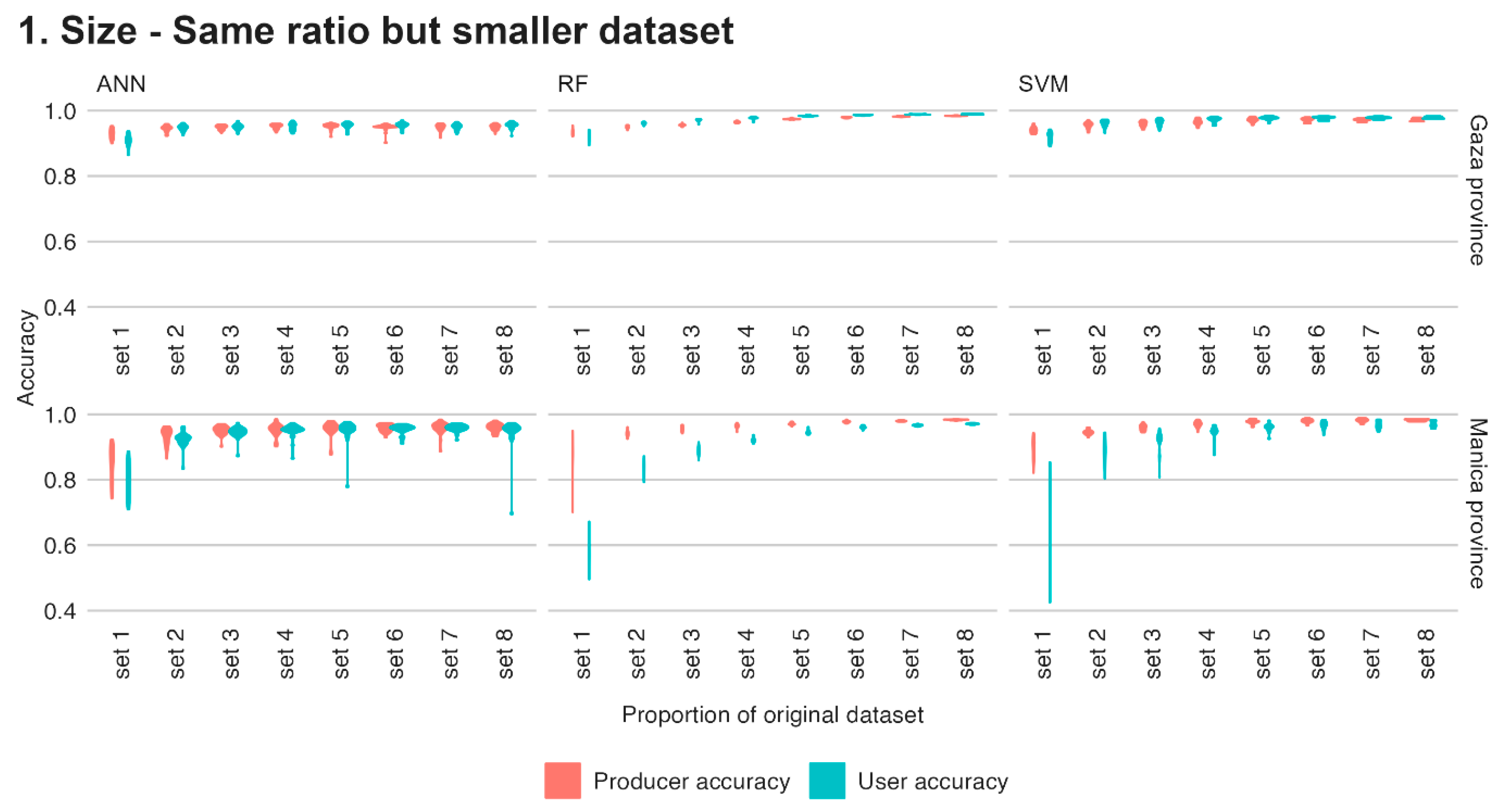
Scenario 1: Size (same ratio, smaller dataset). In this scenario, we investigate the relationship between the amount of training data (TD) and the model’s accuracy. Specifically, we want to determine whether adding more TD in the same ratio always leads to better results or if similar results can be achieved with less data.
To do this, we used eight imbalanced data sets, each with a different proportion of the original training data. The data sets ranged in size from 1% to 100% of the original dataset, with increments of 1, 5, 10, 20, 40, 60, 80, and 100%. The pixel ratio for set 8 of both provinces is shown in
Table 4.
Scenario 2: Balance (equal numbers per class). In this aspect of the study, we will examine the effect of class balance in the training data on the classification results. Simple random sampling often results in class imbalance, where rare classes are under-represented in the training set due to their smaller area. In particular, we will investigate the impact of using larger, balanced datasets on the classification performance.
We used seven sets of balanced data to achieve this, where each class has the same number of TD samples. The first set consists of 50 samples, and the remaining sets will be divided into six equal steps based on the class with the lowest abundance (i.e., the smallest class determines the step sizes). The specific sample sizes (in pixels) for each set are shown in
Table 5.
Scenario 3: Imbalance (over- and undersampling irrigated agriculture). In this scenario, we aim to investigate the effect of class imbalance caused by purposive sampling on the classification performance. Specifically, we will simulate a scenario where the proportion of samples from the class “irrigated agriculture” is increased at the cost of other classes.
To do this, we created nine sets of data, each with a different proportion of “irrigated agriculture” samples. The proportions will be 1%, 5%, 10%, 20%, 50%, 80%, 90%, 95%, and 99%. To ensure that the same total amount of training data is used in each set, the number of samples for the other classes were adjusted accordingly. The remaining training data were divided equally among the other classes, following the method described in [
8] The number of samples in each class for each set is summarized in
Table 6.
Scenario 4: Mislabeling (assigning wrong class labels). In this study, we will examine the effect of mislabeling on the classification accuracy. In smallholder agriculture SSA, class labels can be misassigned due to the heterogeneous nature of the agriculture and the potential for errors or intentional mislabeling.
To simulate this scenario, we created five sets of data, each with a different proportion of mislabeled pixels. The proportions were 1%, 5%, 10%, 20%, and 40%. The focus will be on mislabeling classes that may be considered “border cases” that are likely to be confused, rather than randomly selected classes, following [
1]. These classes are irrigated agriculture, rainfed agriculture, and light vegetation. The number of misclassified pixels is shown in
Table 7.
2.3. Algorithm and Cross-Validation Parameter Tuning
We have used three different algorithms, namely radial support vector machines (SVM), random forests (RF), and artificial neural networks (ANN). For a description of the algorithms, we refer readers to [
11,
30,
31,
32]. We want to illustrate that the algorithms may interpret the data differently and lead to different classifications with different accuracies.
We used the caret package [
33], which uses the free statistical software tool R (version 4.1.2) and allows for systematically comparing different algorithms and composites in a standardized method. We used rf, svmRadial, and nnet algorithms from caret for the random forest, support vector machine, and artificial neural network, respectively.
Cross-validation is a widely used method for evaluating the performance of machine learning algorithms and models. In cross-validation, the data is divided into multiple folds or subsets, typically of equal size. The algorithm is trained on one subset and tested on the other subsets, so each subset is used for testing exactly once. The algorithm’s performance is then evaluated based on the average performance across all the folds.
Spatial K-fold cross-validation is a variation of the traditional cross-validation approach that considers the spatial relationships between the samples in the dataset [
34]. The spatial k-folds method divides the data into k subsets, with each subset consisting of samples that are spatially close to each other. This is particularly useful in remote sensing, where the spatial relationships between the samples are important in understanding the underlying patterns in the data. In this study, we used spatial k-fold cross-validation.
2.4. Classifications and Replications
To ensure the accuracy and reliability of our models, we conducted 25 iterations of all steps for each of the three algorithms using the same seed numbers. By replicating the process, we could account for the variability in accuracies that may depend on the specific training data sets used in each run. This allowed us to evaluate the robustness and generalizability of the models and determine whether they were sensitive to specific training data points and seed numbers or whether they were more robust and generalizable to the study area.
We created various sample sizes and compositions by using random subsampling from the complete sample set, with different seed values. To decrease computation time, we used the caret::train() function and included all variables in the model rather than using forward feature selection of the variables.
Figure 3 displays the range of model parameter values per scenario, training data set, and province based on the overall accuracy. The range of values used by the same algorithms across different seed values and scenarios demonstrates the inherent randomness in the model results, even with the same training data. Some parameter values, such as the mtry value of 2 for RF and the decay and size values for ANN, consistently show higher preference across all datasets. However, sigma from SVM exhibits little overlap between the provinces and scenarios. These findings suggest that parameter tuning is highly recommended for SVM and ANN while less necessary for rf, as evident from the lack of clear patterns in the results—similar to what [
35] also found.
2.5. Accuracy Assessment
We calculated the overall accuracy and the user’s and producer’s accuracies using the same validation dataset for each iteration (
Table 8).
4. Discussion
The results of this study align with previous research by [
11], which found that larger sample sizes lead to improved classifier performance and that increasing the sample set size after a certain point did not substantially improve the classification accuracy. Scenarios 1 and 2 in this research show that larger datasets improve overall classification results, but not by much. This plateauing of overall accuracy is not unexpected, as when classifications reach very high overall accuracy, there is little potential for further increases. Our study is also in line with the results of [
11], in that user and producer accuracies continued to increase with larger sample sizes, indicating that larger sample sizes are still preferable to smaller sizes, even with similar overall accuracy results.
A large spread in accuracy means that the specific results depend more on the dataset that is used for that classification than other factors. For example, the SVM algorithm in Manica in Scenario 1 resulted in a user accuracy of just above 40%, but also 85%. By chance, any of the two could have become the final classification; if it was the 85% classification, one would think enough data was collected for the study, whereas the other sets show that higher accuracies are possible, with less spread in values. The lower spread in values also indicates a more stable model which can generalize more. It also means that the specific dataset used for the classification is less important, as similar results can be expected from any random subset, also seen in
Section 3.3.
Scenario 1, where eight datasets ranging in size from 1% to 100% of the original dataset were used, shows that larger training datasets lead to higher user and producer accuracy with less spread in values (
Figure 5). The size of set 5 in Manica falls between sets 3 and 4 of Gaza (40% vs. 10–20%, respectively), which are also the sets after which the accuracies plateau in Gaza. This corresponds to ~1300 pixels of irrigated agriculture for Manica and ~1900–3900 for Gaza. This reinforces the statement that larger training data sets are preferable over smaller sets but that there is an optimum after which accuracies only marginally increase at the cost of more computing time and, effectively, more resources are ‘lost’ collecting that data in the first place. To find out if enough data is collected for a classification of irrigated area, researchers and practitioners can use this subsetting method to evaluate if different iterations yield the same, stable results, or if additional resources should be put towards more field data collection.
Scenario 2 also examines the impact of data size on classification performance, but with equal numbers of samples per class, spread over seven sets. Similar to scenario 1, larger datasets generally result in higher user and producer accuracies (
Figure 6). However, this scenario highlights differences in the performance of the classifiers in the two study areas. In scenario 1, the results of both study areas followed similar patterns but with different accuracy values. In this scenario, however, the user and producer accuracy trends are reversed, depending on the study area. In Gaza, the user’s accuracy is consistently lower than the producer’s, whereas in Manica, the user’s accuracy is consistently higher than the producer’s. Manica also shows a larger spread in values for both user and producer accuracy.
This trend reversal suggests that the models in Gaza are better able to classify the non-irrigated agriculture classes than the irrigated agriculture class, indicating a more generalized model. Conversely, the Manica models can better classify the irrigated agriculture class than the non-irrigated agriculture classes, indicating a less generalized model. As all classes have the same number of pixels per dataset within the same study area, the complexity of the landscape likely plays a role in this difference. The two provinces generally have different landscapes (flat vs. mountain), climate (little vs. much rainfall) and consequently, different agricultural practices, with different field sizes (larger vs. small) and shapes (regular vs. irregular). It is worth noting that, even though Gaza has twice the number of pixels as Manica, sets 1 are the same size in both cases, and 3 of Gaza and 7 of Manica are similar in size. However, even for these sets with similar sizes, Gaza has higher producer accuracies, and Manica has higher user accuracies.
Scenario 3, where irrigated agriculture is vastly over- and undersampled in nine sets ranging from 1% to 99%, shows a peak in overall accuracy around sets 3 and 4 (
Figure 4Error! Reference source not found., 10% and 20% irrigated agriculture in the dataset). These two sets reflect the ‘true’ composition of the dataset, which was found in the field. When irrigated agriculture is underrepresented (sets 1 and 2, 1% and 5%), the overall accuracy is not much lower. This is because the other majority classes have a greater impact on the overall accuracy. As more irrigated agriculture is present in the training datasets (sets 5 to 9, 50–99%), the other classes decrease in size, and irrigated agriculture becomes the majority class. The high user accuracy (
Figure 7) indicates that any irrigated agriculture in the validation set is correctly classified (not surprising as all pixels are classified as such). However, the reverse is that the producer accuracy is extremely low (many of the pixels are wrongly classified as irrigated agriculture instead of a different class).
Scenario 4, where similar classes are mislabeled on purpose in five sets from 1% to 40% mislabeling, shows a decrease in overall accuracy (
Figure 4) for ANN and only a minor decrease in the last set for RF. SVM does not seem to be affected, possibly because the support vectors used for distinguishing the different classes do not change much between the sets, indicating that SVM is less sensitive to data set compositions.
The user and producer accuracies (
Figure 8) also show that SVM can handle this imbalance, perhaps because it uses the same support vectors to distinguish the different classes in all the sets. Adding more data will not help the algorithm, as that data is not near the separation planes between classes. RF is similarly stable, except for the last set, which also shows a larger spread in accuracy values. The user accuracy is also higher than the producer’s, which comes from slowly oversampling irrigated agriculture (among other classes). The ANN has many difficulties with changing compositions, as seen from the large spread in values and decreased accuracies. Overall, RF and SVM seem to handle this mislabeled data well.
The results of the study demonstrate the importance of the dataset and algorithm selection in accurately classifying irrigated agriculture in remote sensing data. Visual inspection reveals that different areas are classified as irrigated agriculture depending on the dataset and algorithm used. In some cases, the models prioritize farmer-led irrigated areas over more conventional large-scale irrigated areas, but the latter is generally classified more accurately. The amount of data used and the balance between classes also have a significant impact on the accuracy of classification, with too few data or imbalanced data resulting in underestimation of the extent of farmer-led irrigation, and too much noise resulting in overestimation. The RF and SVM algorithms are found to be more robust with noisy data than the ANN algorithm. Although the maps do not distinguish between farmer-led irrigation and large-scale irrigation, our knowledge of the area enables us to interpret the maps in terms of these different types of irrigation.
Generally, there are many oversampling and undersampling strategies which have not been tested. The focus of this study was not to find the best method to deal with imbalanced data, but to illustrate what imbalanced data does with the final results.
Overall, ANN showed high results but with a large spread in all scenarios and study areas. The RF and SVM showed results similar to each other, depending on the scenario’s dataset and study area, resulting in higher accuracies with lower spreads. Both are recommended for mapping irrigated agriculture. The large spread in ANN shows that it may be suitable for detecting irrigated agriculture, but only in certain circumstances—when there is much data (scenario 1 final sets), and the landscape is more homogeneous (Gaza, all scenarios). Nevertheless, the random chance of high or low accuracies is higher with ANN than with RF and SVM (i.e., larger spread), indicating that the specific dataset used in modelling is more important for ANN than the other two algorithms.
According to [
31], the training sample size and quality can have a greater impact on classification accuracy than the choice of algorithm. As a result, differences in accuracy between datasets within the same algorithm should be more pronounced than those between different algorithms. This is supported by scenarios 1, 2, and 3, where the algorithms show similar trends and values but exhibit greater variability within datasets. Scenario 3 demonstrates that user and producer accuracies may cross over, but the differences between datasets are still more significant than those between algorithms. However, scenario 4 is less conclusive, since there is little variation in the high accuracies of the RF and SVM algorithms across all sets, with some variation in Manica. At the same time, ANN shows dissimilar trends and greater differences between sets compared to the other two algorithms.


