
Simulation of Compact Spaceborne Lidar with High-Repetition-Rate Laser for Cloud and Aerosol Detection under Different Atmospheric Conditions
 , ,
, ,
Abstract
:1. Introduction
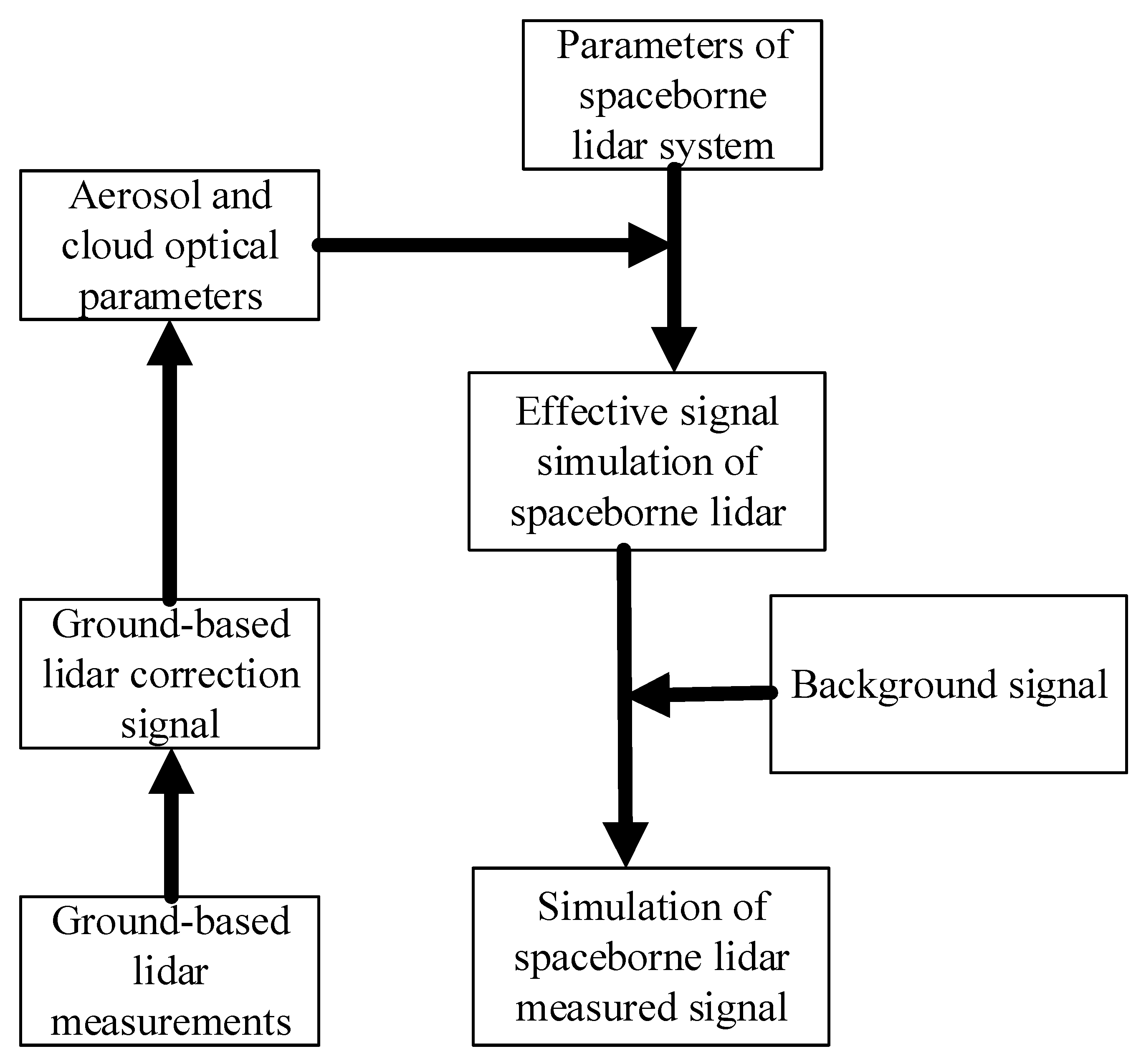
2. Simulation Process
- (1)
- Based on the measurement data of the ground-based lidar, the correction signal of the ground-based lidar system was obtained by background deduction, distance correction, geometric factor correction, and noise smoothing data in sequence;
- (2)
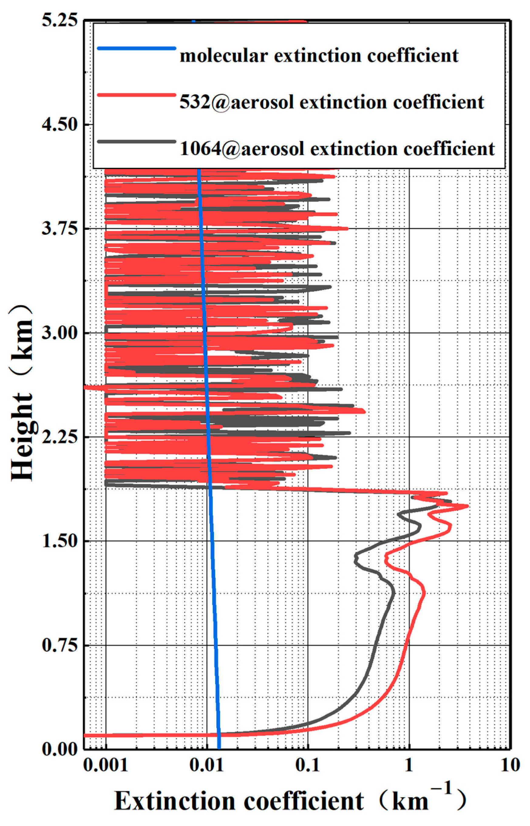
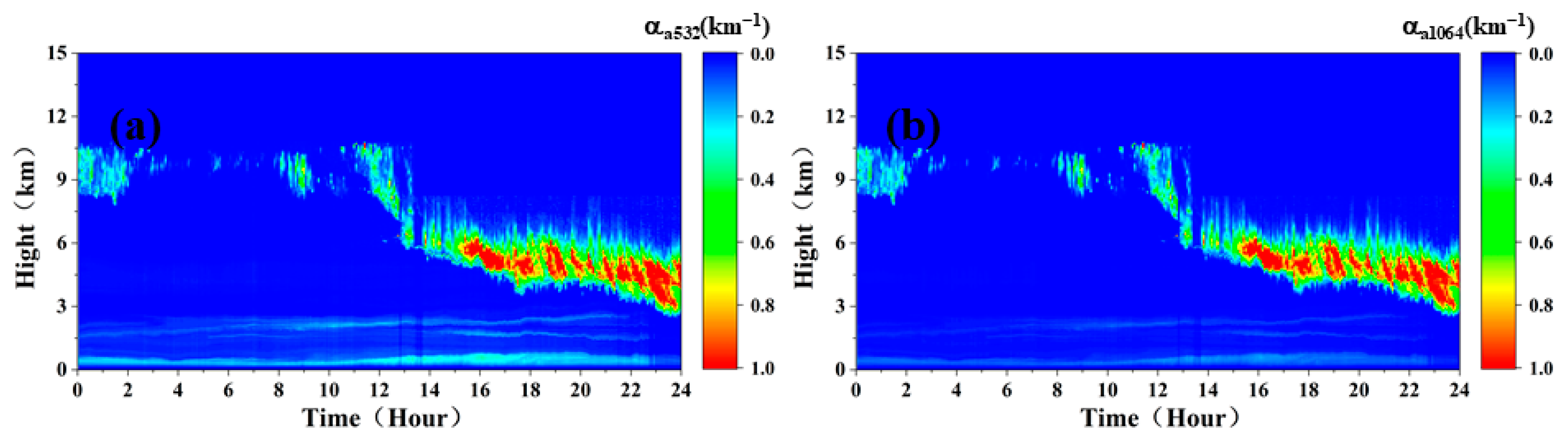
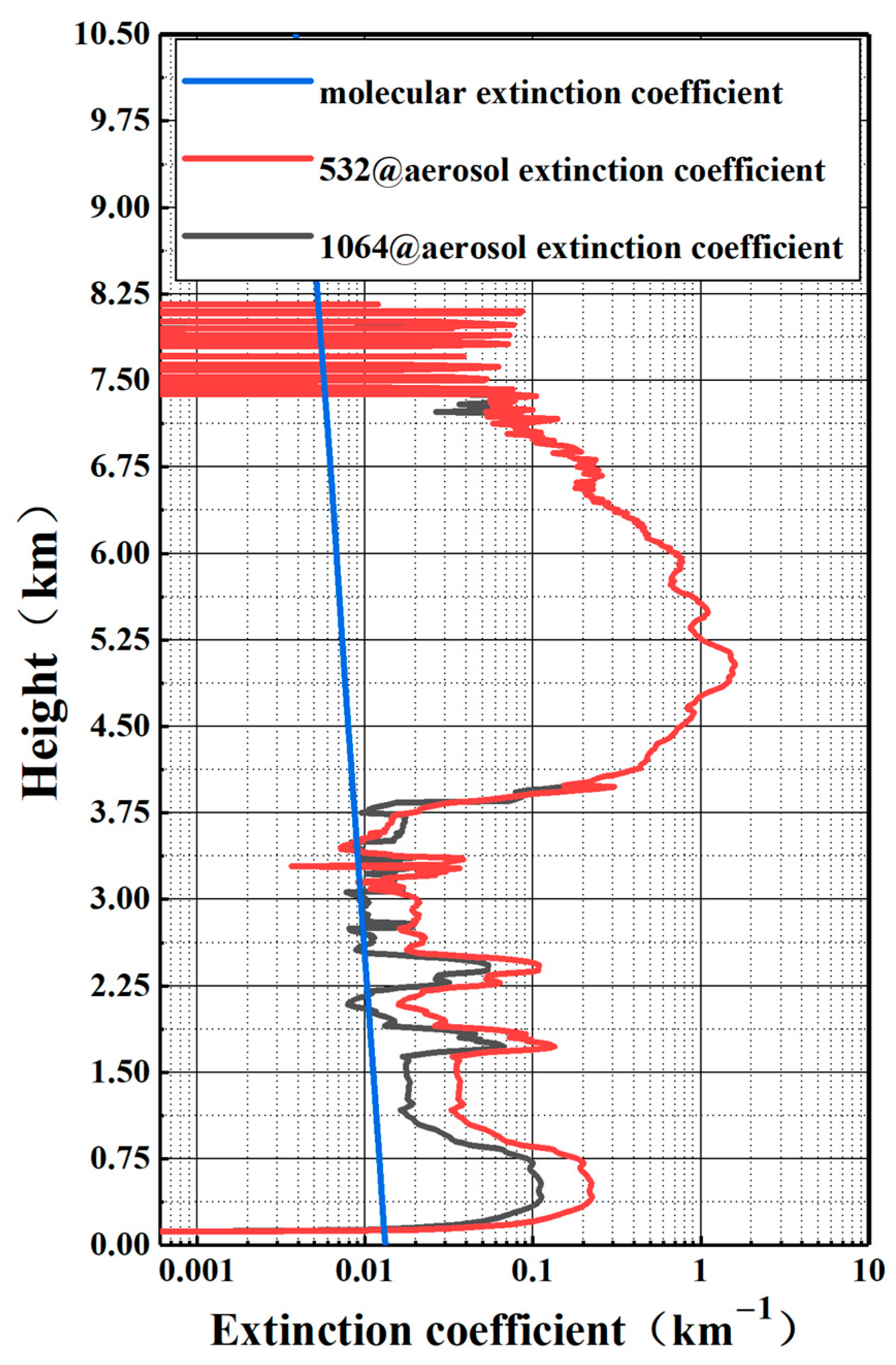
- The backscattering ratio, extinction, and backscattering coefficients of atmospheric aerosol and cloud particles under different atmospheric conditions were obtained by the aerosol and cloud inversion algorithm;
- (3)
- Based on spaceborne lidar system parameters, ground-based lidar inversion of aerosol and cloud particles’ optical parameters, and the spaceborne lidar signal simulation algorithm, the spaceborne lidar atmospheric echo effective signal was simulated;
- (4)
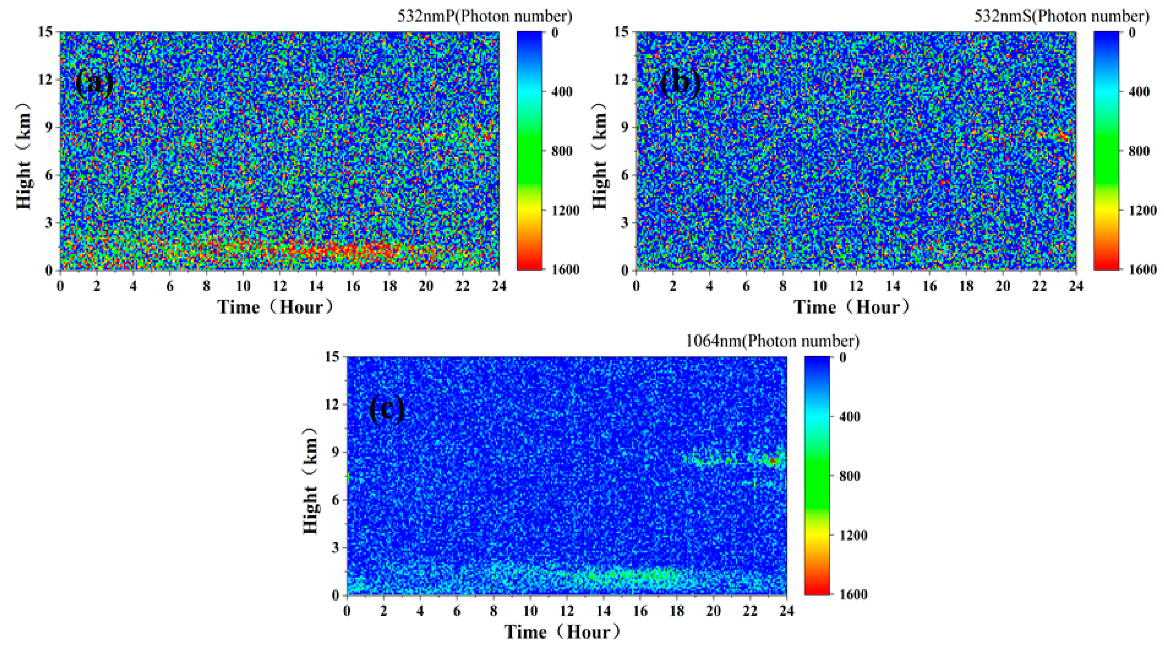
- Through the spaceborne lidar system parameters and atmospheric background data, the noise signal of the simulation system was simulated and superimposed on the effective signal, and finally, the actual measurement signals of the spaceborne lidar with background and its signal-to-noise ratio (SNR) were obtained.
2.1. Simulation of the Effective Signal of Spaceborne Lidar Based on Ground-Measured Signal
2.1.1. Inversion of Optical Parameters of Ground-Based Lidar
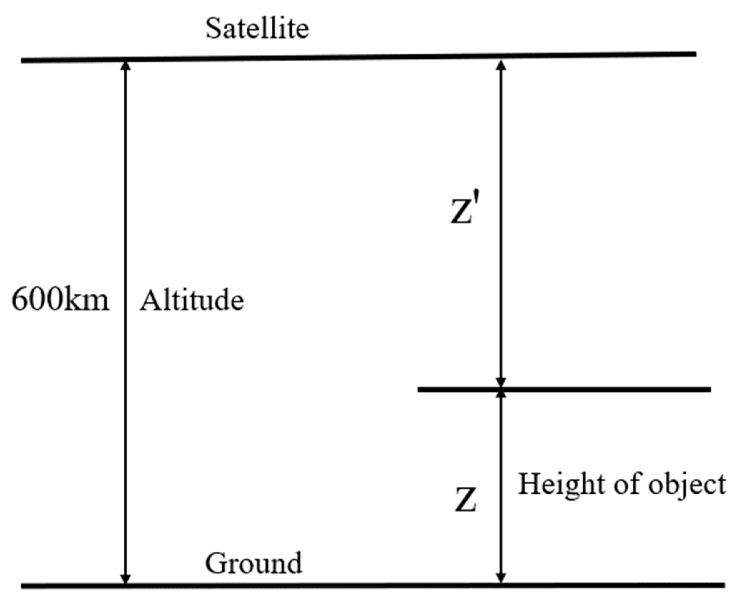
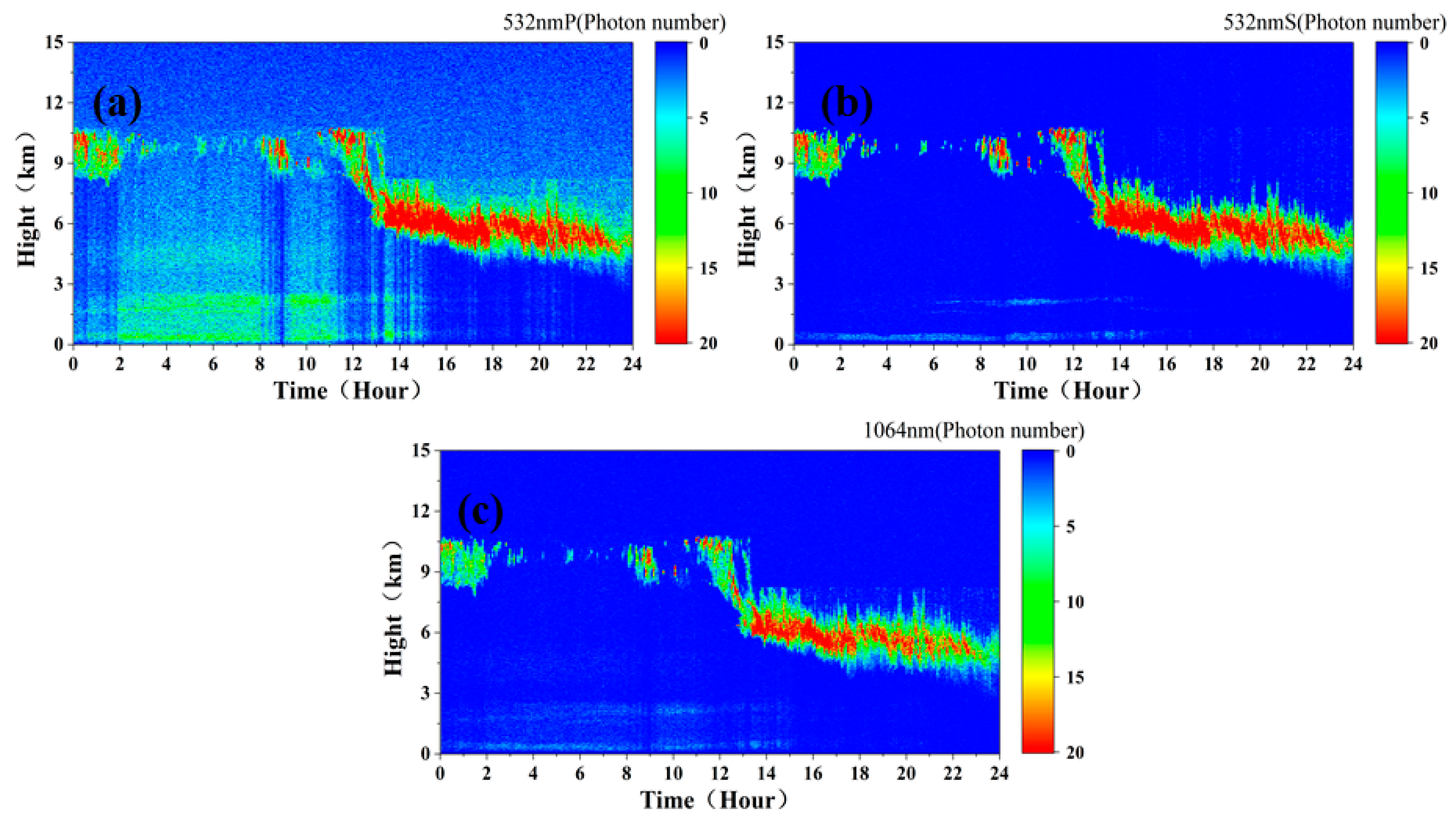
2.1.2. Simulation of Effective Signals of Spaceborne Lidar
2.2. Simulation of Background Signal and Noise of Spaceborne Lidar
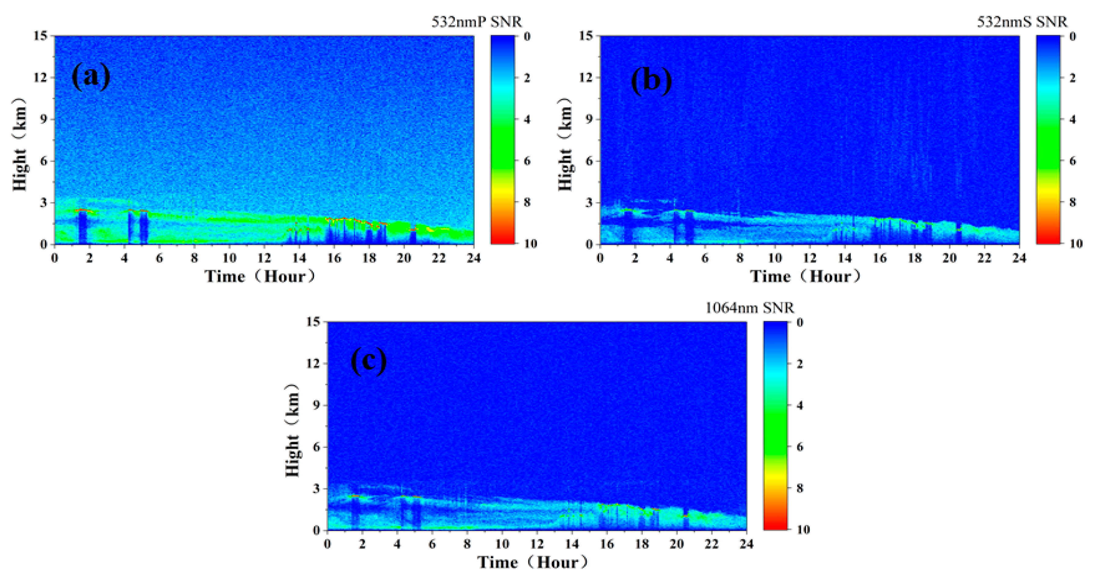
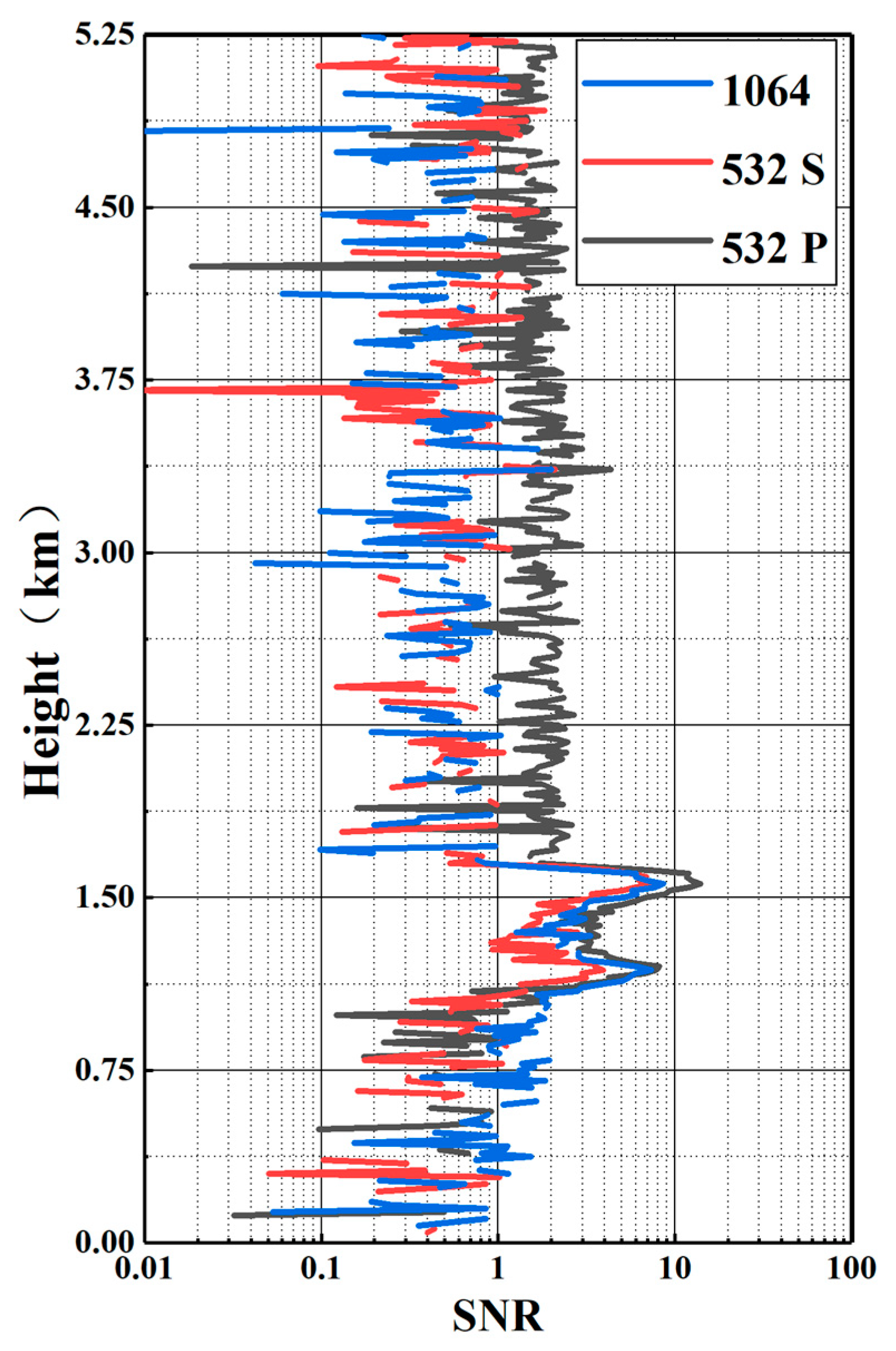
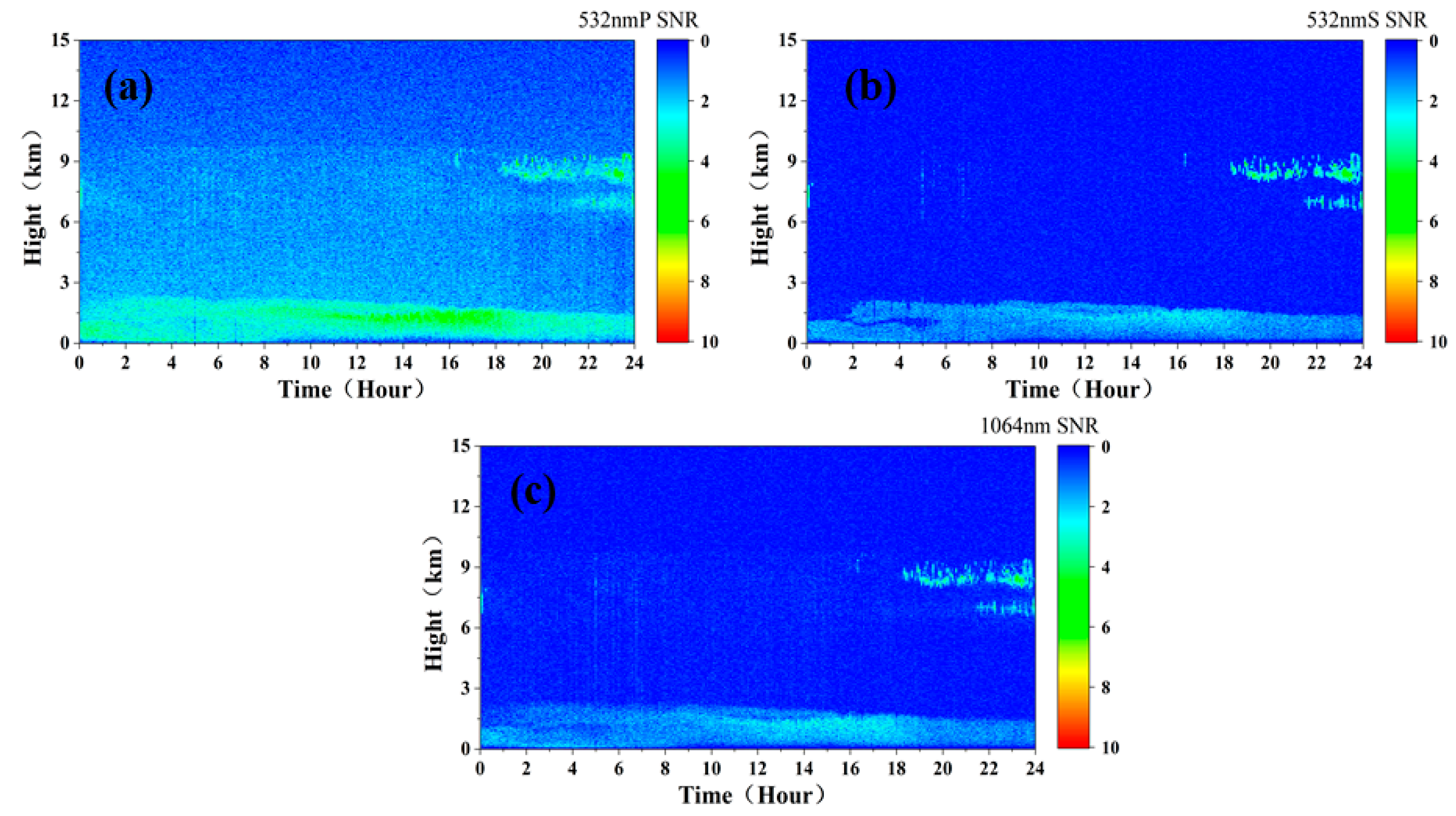
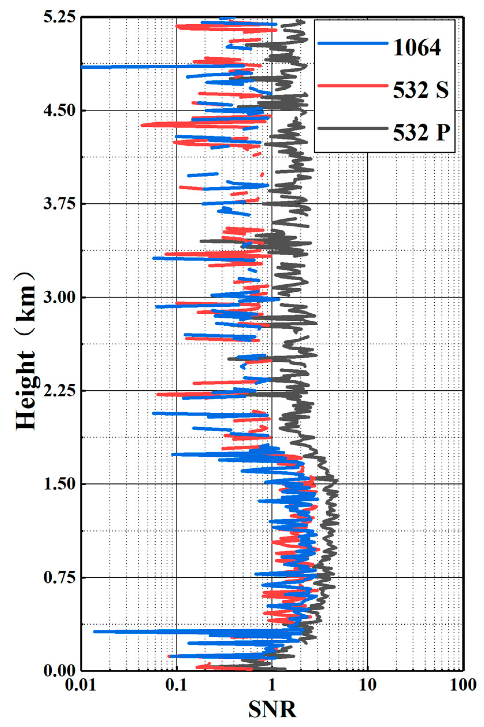
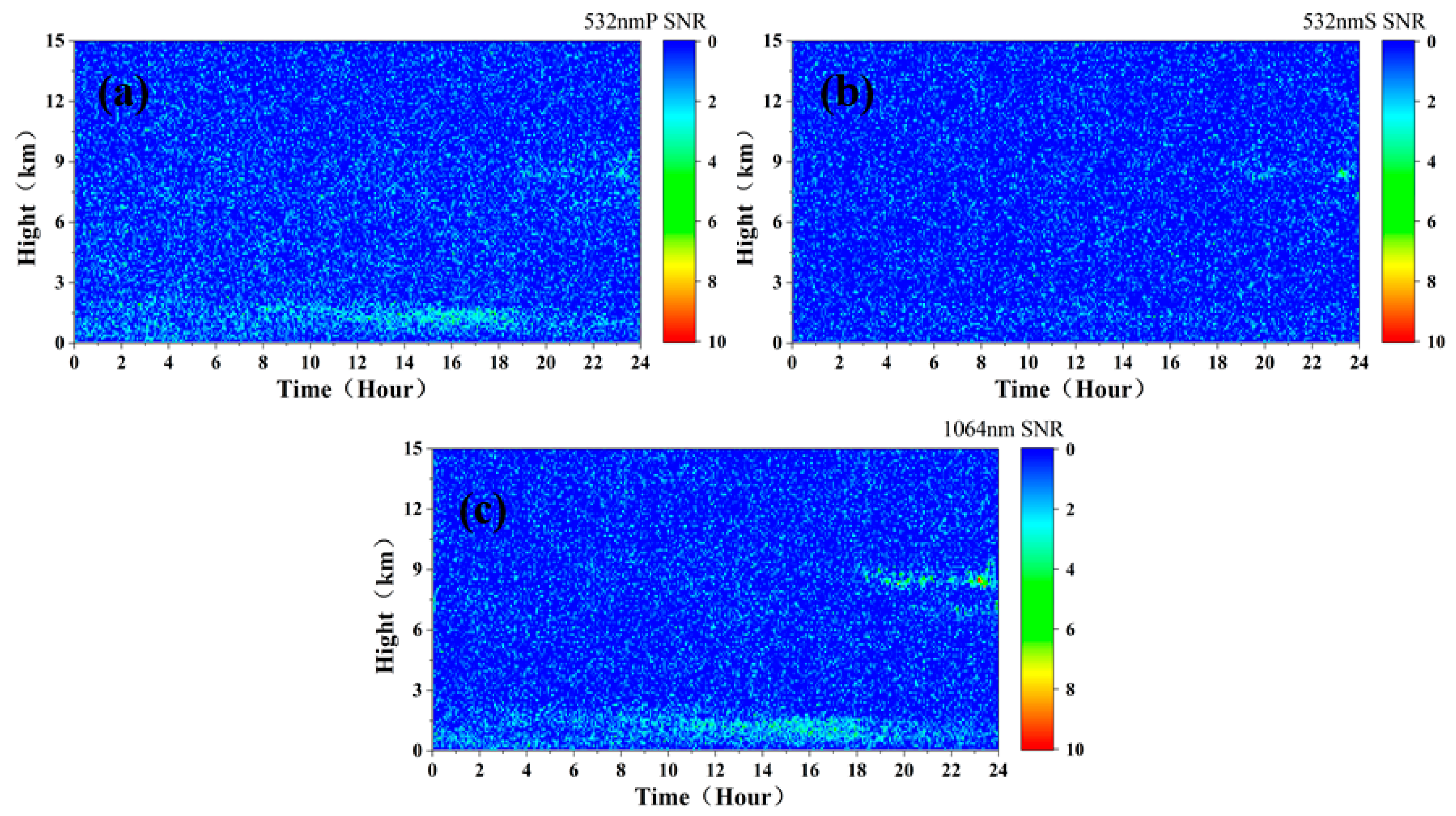
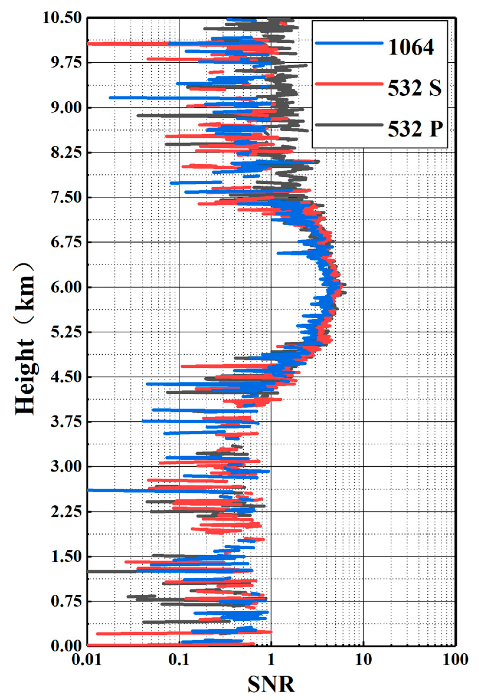
2.3. Simulation of the Signal-to-Noise Ratio of Spaceborne Lidar Signal
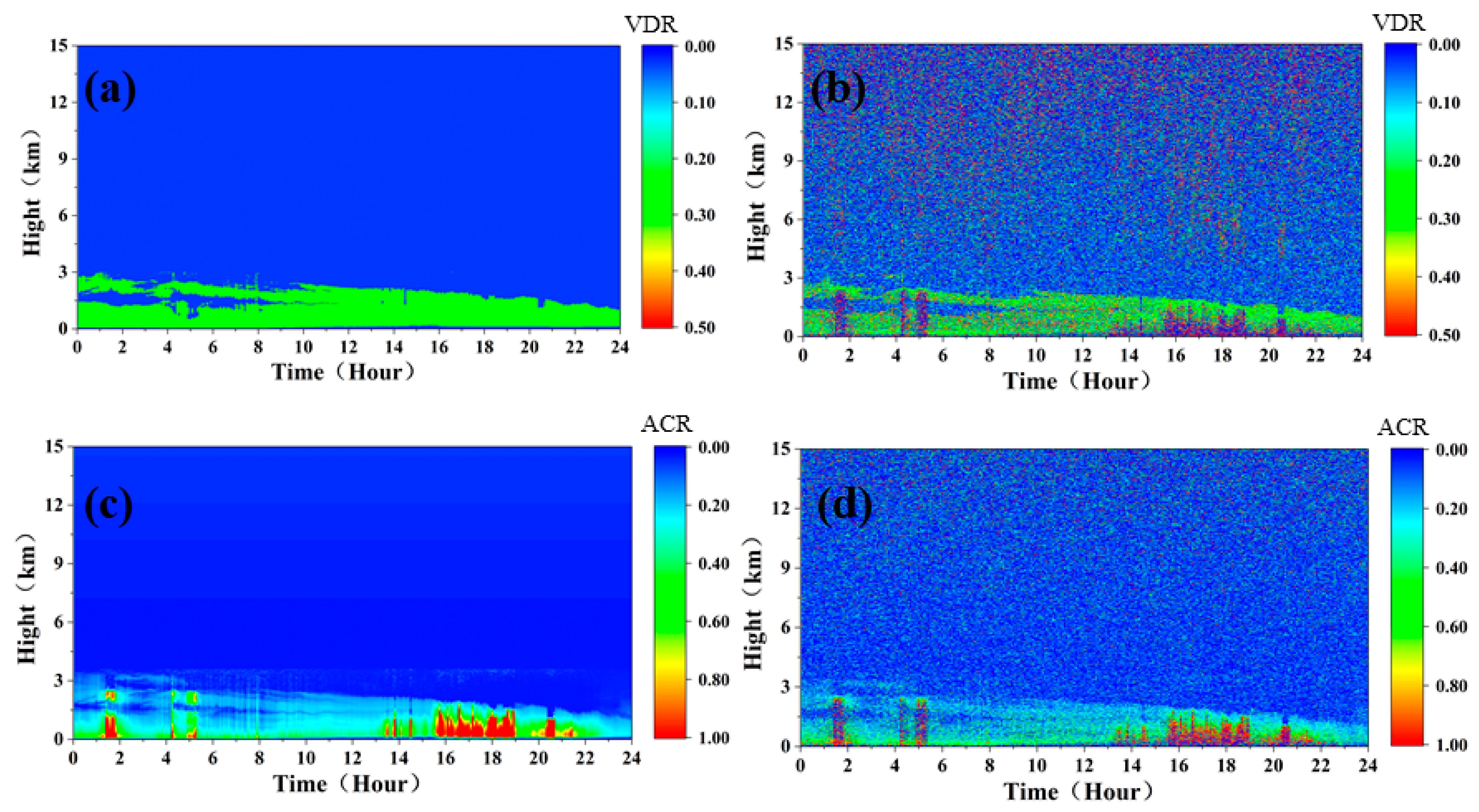
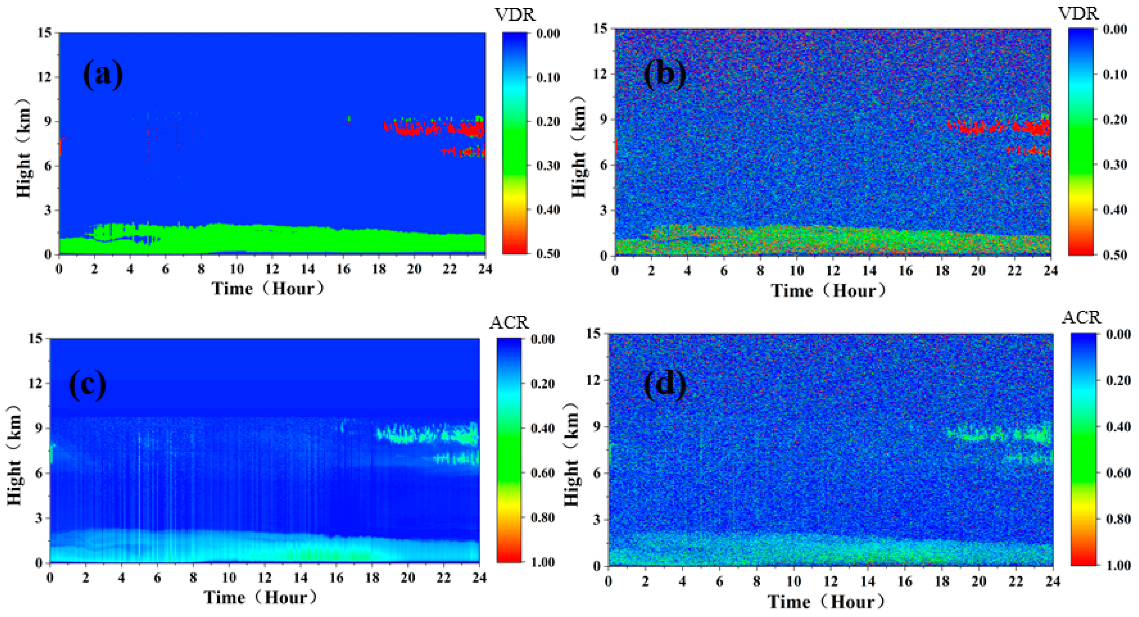
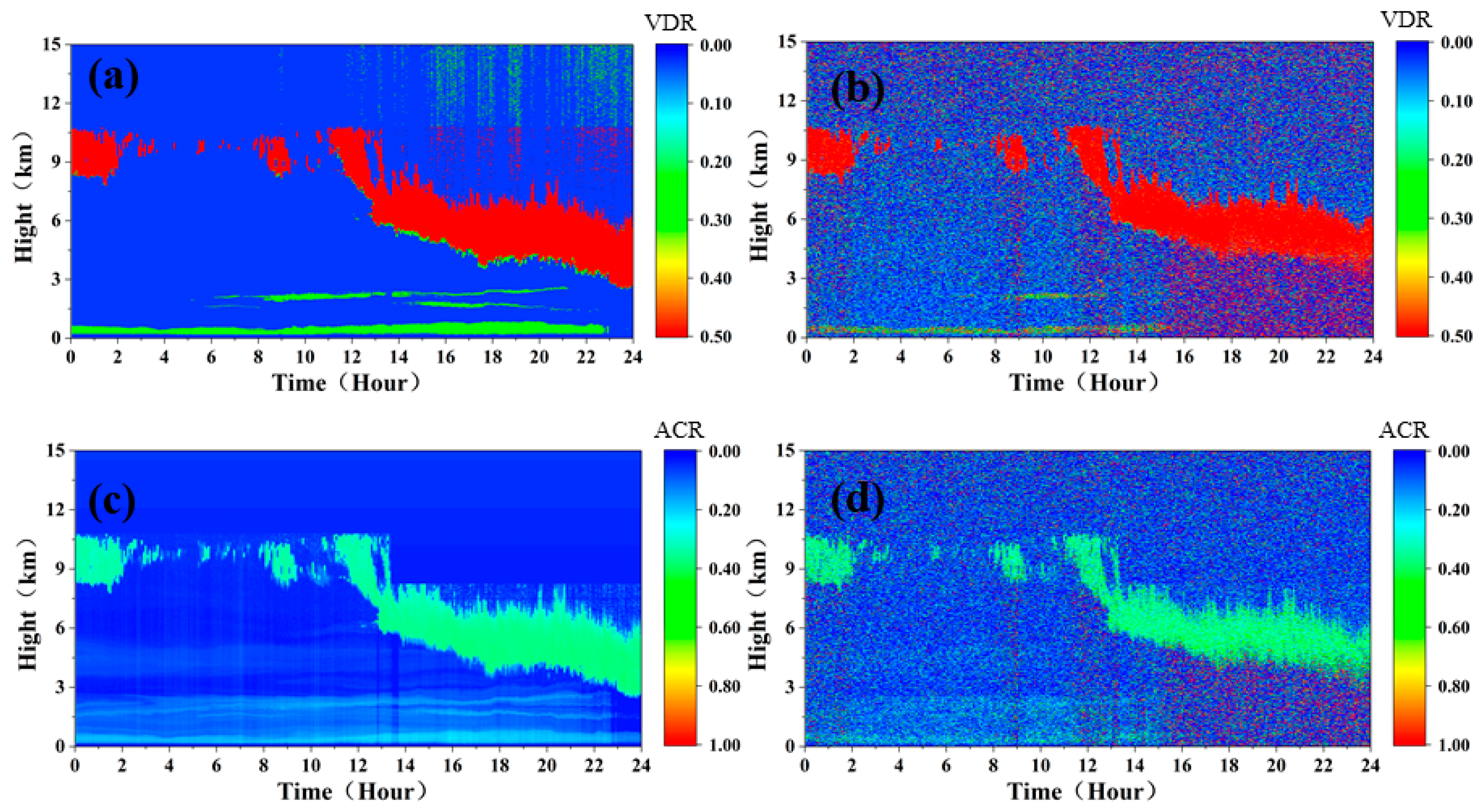
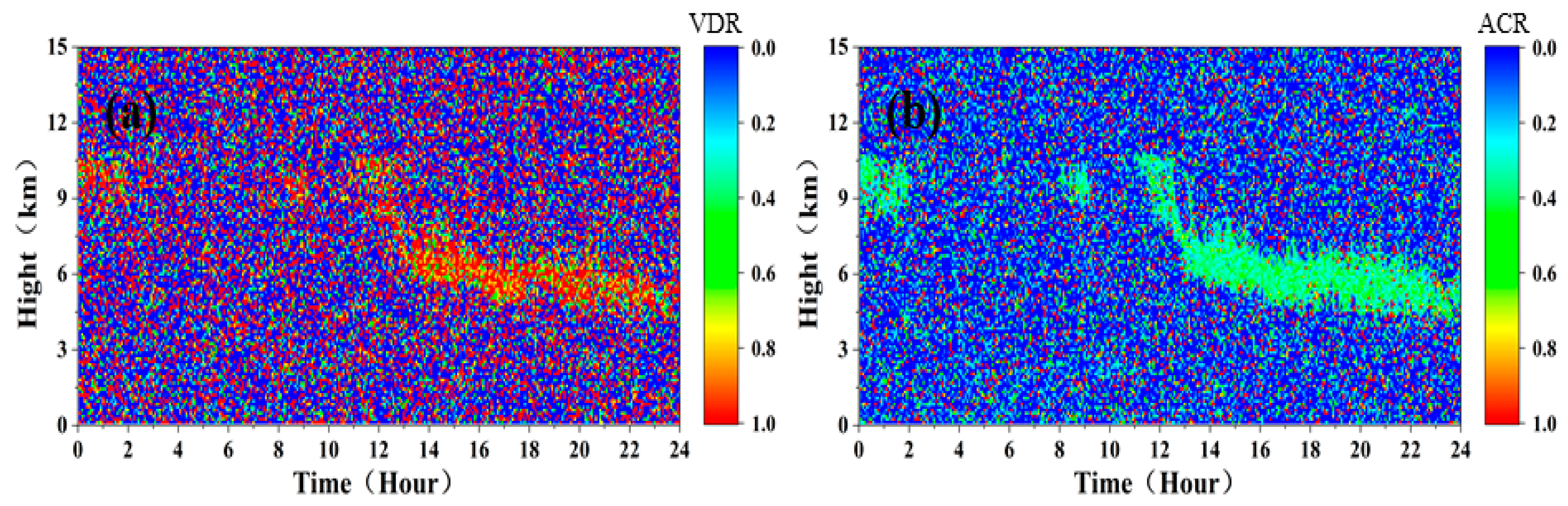
2.4. Simulation of the VDR and ACR
3. Simulation Results
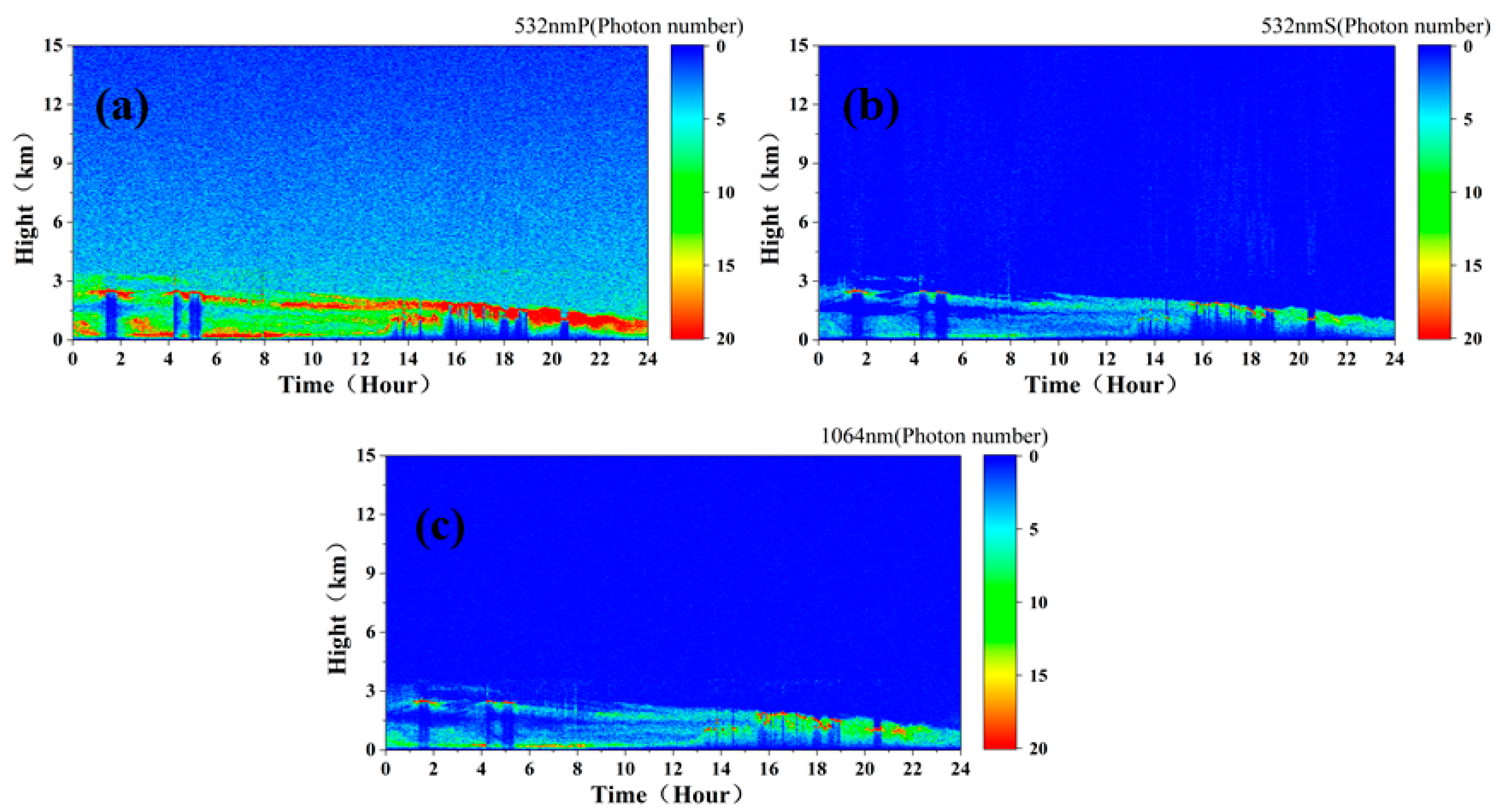
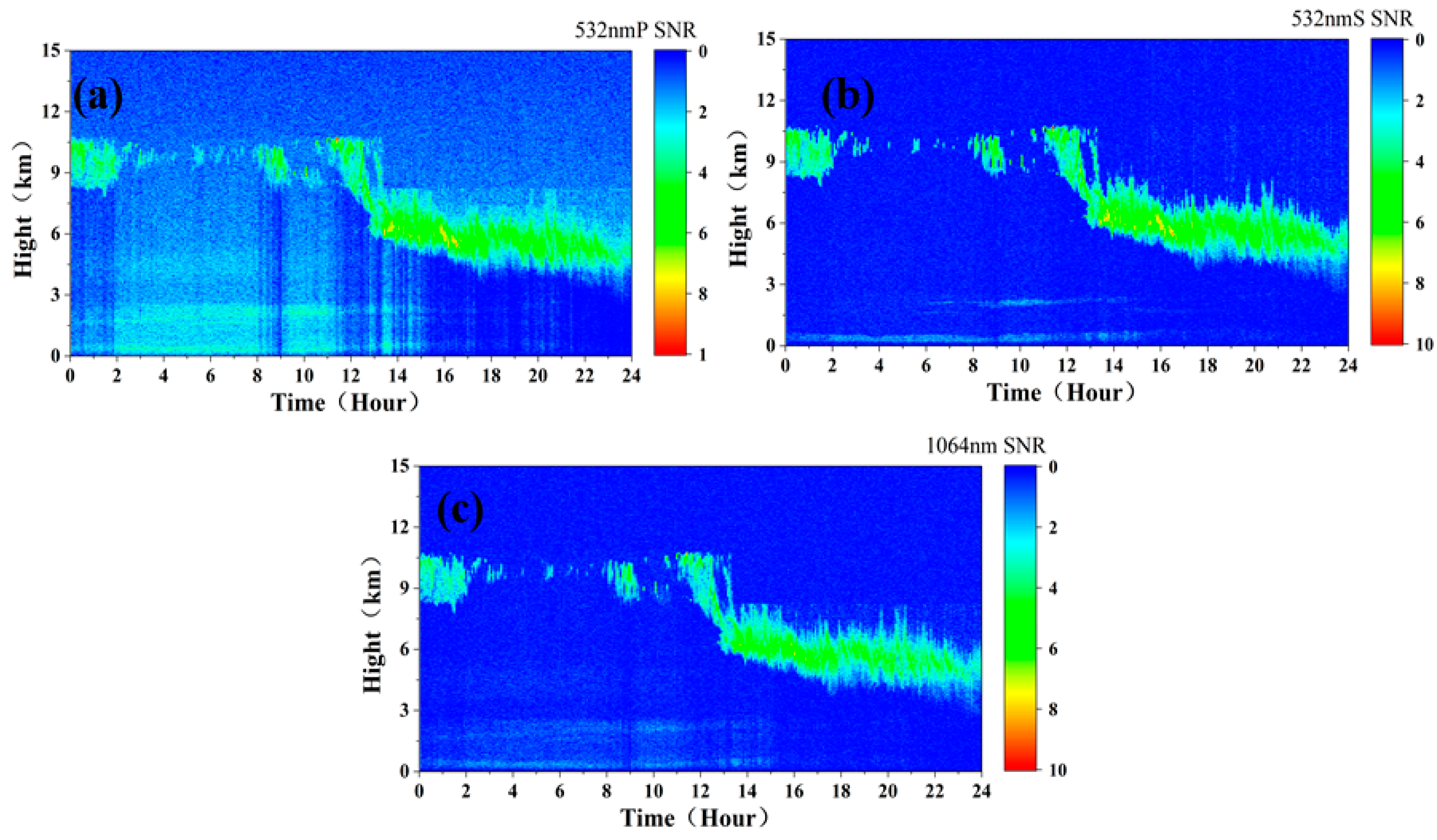
3.1. Simulation of Heavy-Pollution Low-Cloud Atmosphere
3.1.1. Observation Model at Night
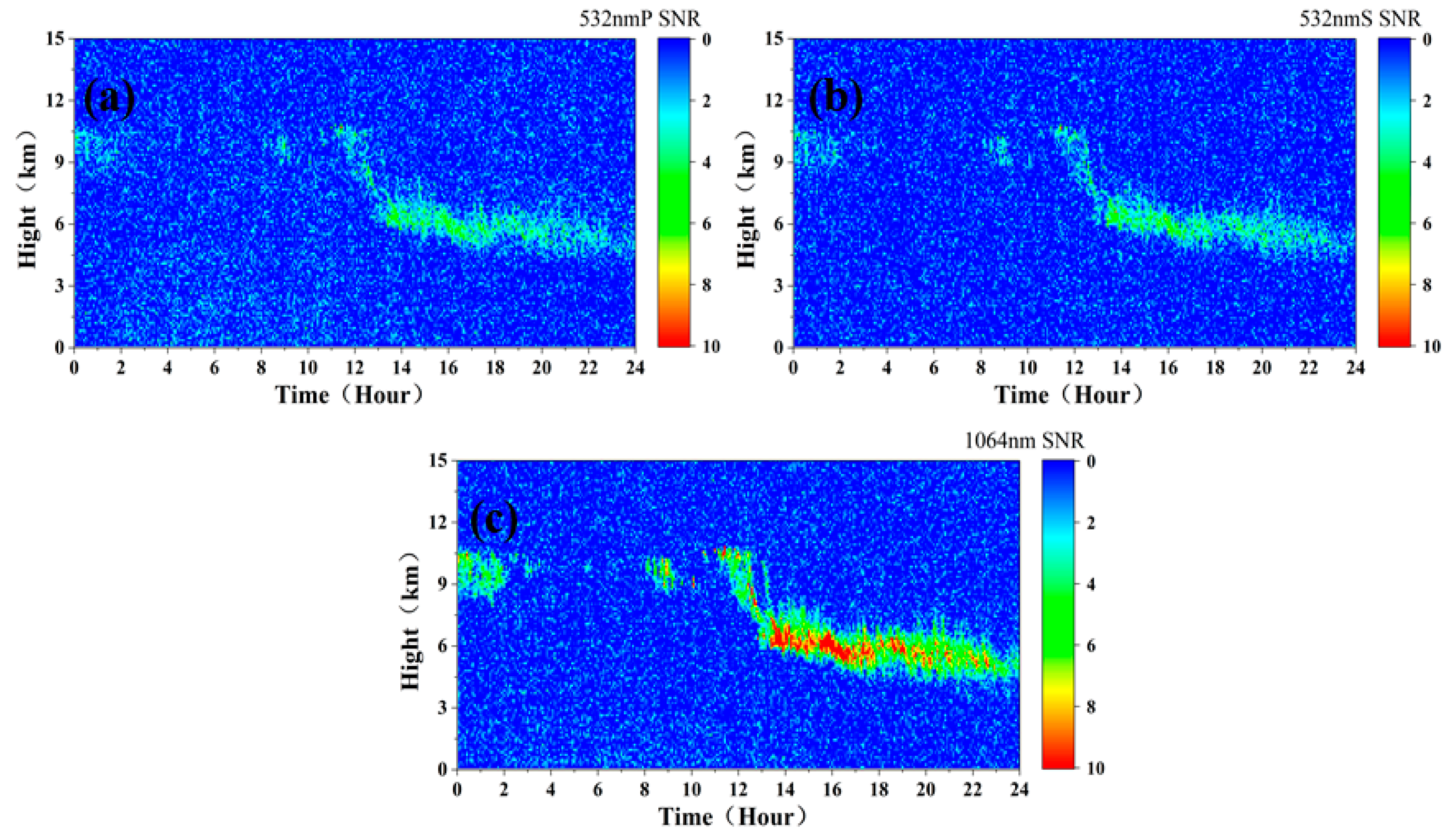
3.1.2. Observation Model in Daytime
3.2. Simulation of Moderate-Pollution and High-Cloud Atmosphere
3.2.1. Observation Model at Night
3.2.2. Observation Model in Daytime
3.3. Simulation of a Clear and Cloudy Day
3.3.1. Observation Model at Night
3.3.2. Observation Model in Daytime
4. Conclusions
Author Contributions
Funding
Data Availability Statement
Acknowledgments
Conflicts of Interest
References
- Gunaseelan, I.; Bhaskar, V. In Aerosols and Clouds Interactions in an Urban Atmosphere. In Proceedings of the 29th International Laser Radar Conference (ILRC), Hefei, China, 24–28 June 2019. [Google Scholar]
- Eck, T.F.; Holben, B.N.; Reid, J.S.; Xian, P.; Giles, D.M.; Sinyuk, A.; Smirnov, A.; Schafer, J.S.; Slutsker, I.; Kim, J.; et al. Observations of the Interaction and Transport of Fine Mode Aerosols with Cloud and/or Fog in Northeast Asia from Aerosol Robotic Network and Satellite Remote Sensing. J. Geophys. Res.-Atmos. 2018, 123, 5560–5587. [Google Scholar] [CrossRef]
- Brooks, S.D.; Thornton, D.C.O. Marine Aerosols and Clouds. In Annual Review of Marine Science; Carlson, C.A., Giovannoni, S.J., Eds.; Annual Reviews: San Mateo, CA, USA, 2018; Volume 10, pp. 289–313. [Google Scholar]
- Seinfeld, J.H.; Bretherton, C.; Carslaw, K.S.; Coe, H.; DeMott, P.J.; Dunlea, E.J.; Feingold, G.; Ghan, S.; Guenther, A.B.; Kahn, R.; et al. Improving our fundamental understanding of the role of aerosol-cloud interactions in the climate system. Proc. Natl. Acad. Sci. USA 2016, 113, 5781–5790. [Google Scholar] [CrossRef] [Green Version]
- Wang, Y.J.; Sun, L.; Liu, D.; Wang, Z.; Wang, Z.Z.; Xie, C.B. In Cloud and Aerosol Interaction Observed in Skynet Hefei Site in China. In Proceedings of the 27th International Laser Radar Conference (ILRC), New York, NY, USA, 5–10 July 2015; Natl Ocean & Atmospher Adm, Cooperat Remote Sensing Sci & Technol Ctr.: New York, NY, USA, 2015. [Google Scholar]
- Kay, J.E.; L’Ecuyer, T.; Chepfer, H.; Loeb, N.; Morrison, A.; Cesana, G. Recent Advances in Arctic Cloud and Climate Research. Curr. Clim. Chang. Rep. 2016, 2, 159–169. [Google Scholar] [CrossRef] [Green Version]
- Belikov, Y.E.; Dyshlevsky, S.V.; Repin, A.Y. Effect of Thin High Clouds and Aerosol Layers on the Heating and Dissipation of Low-level Clouds in the Arctic. Russ. Meteorol. Hydrol. 2021, 46, 245–255. [Google Scholar] [CrossRef]
- Hartmann, D.L. Tropical anvil clouds and climate sensitivity. Proc. Natl. Acad. Sci. USA 2016, 113, 8897–8899. [Google Scholar] [CrossRef] [Green Version]
- Scott, C.E.; Arnold, S.R.; Monks, S.A.; Asmi, A.; Paasonen, P.; Spracklen, D.V. Substantial large-scale feedbacks between natural aerosols and climate. Nat. Geosci. 2018, 11, 44. [Google Scholar] [CrossRef] [Green Version]
- Schafer, B.; Carlsen, T.; Hanssen, I.; Gausa, M.; Storelvmo, T. Observations of cold-cloud properties in the Norwegian Arctic using ground-based and spaceborne lidar. Atmos. Chem. Phys. 2022, 22, 9537–9551. [Google Scholar] [CrossRef]
- Dionisi, D.; Brando, V.E.; Volpe, G.; Colella, S.; Santoleri, R. Seasonal distributions of ocean particulate optical properties from spaceborne lidar measurements in Mediterranean and Black sea. Remote Sens. Environ. 2020, 247, 111889. [Google Scholar] [CrossRef]
- Gupta, G.; Ratnam, M.V.; Madhavan, B.L.; Prasad, P.; Narayanamurthy, C.S. Vertical and spatial distribution of elevated aerosol layers obtained using long-term ground-based and space-borne lidar observations. Atmos. Environ. 2021, 246, 118172. [Google Scholar] [CrossRef]
- Chanin, M.L.; Hauchecorne, A.; Malique, C.; Nedeljkovic, D.; Blamont, J.E.; Desbois, M.; Tulinov, G.; Melnikov, V. First results of the ALISSA lidar on board the MIR platform. Comptes Rendus De L’academie Des Sci. Ser. IIA Earth Planet. Sci. 1999, 328, 359–366. [Google Scholar]
- Hu, Y.X.; Vaughan, M.; Liu, Z.Y.; Lin, B.; Yang, P.; Flittner, D.; Hunt, B.; Kuehn, R.; Huang, J.P.; Wu, D.; et al. The depolarization-attenuated backscatter relation: CALIPSO lidar measurements vs. theory. Opt. Express 2007, 15, 5327–5332. [Google Scholar] [CrossRef] [PubMed]
- Burton, S.P.; Ferrare, R.A.; Vaughan, M.A.; Omar, A.H.; Rogers, R.R.; Hostetler, C.A.; Hair, J.W. Aerosol classification from airborne HSRL and comparisons with the CALIPSO vertical feature mask. Atmos. Meas. Tech. 2013, 6, 1397–1412. [Google Scholar] [CrossRef] [Green Version]
- Winker, D.M.; Hunt, W.; Hostetler, C. In Status and performance of the CALIOP lidar. In Proceedings of the Conference on Laser Radar Techniques for Atmospheric Sensing, Maspalomas, Spain, 14–16 September 2004; pp. 8–15. [Google Scholar]
- Powell, K.A. The Development of the CALIPSO LiDAR Simulator. Master’s Thesis, The College of William and Mary ProQuest Dissertations Publishing, Williamsburg, VA, USA, 2005; p. 1539626831. [Google Scholar]
- Stoffelen, A.; Pailleux, J.; Kallen, E.; Vaughan, J.M.; Isaksen, L.; Flamant, P.; Wergen, W.; Andersson, E.; Schyberg, H.; Culoma, A.; et al. The atmospheric dynamics mission for global wind field measurement. Bull. Am. Meteorol. Soc. 2005, 86, 73. [Google Scholar] [CrossRef]
- Winker, D.M.; Couch, R.H.; McCormick, M.P. An overview of LITE: NASA’s lidar in-space technology experiment. Proc. IEEE 1996, 84, 164–180. [Google Scholar] [CrossRef]
- Couch, R.H.; Rowland, C.W.; Ellis, K.S.; Blythe, M.P.; Regan, C.P.; Koch, M.R.; Antill, C.W.; Kitchen, W.L.; Cox, J.W.; Delorme, J.F.; et al. Lidar in-Space Technology Experiment (Lite)-Nasas 1st in-Space Lidar System for Atmospheric Research. Opt. Eng. 1991, 30, 88–95. [Google Scholar] [CrossRef]
- Proestakis, E.; Amiridis, V.; Marinou, E.; Binietoglou, I.; Ansmann, A.; Wandinger, U.; Hofer, J.; Yorks, J.; Nowottnick, E.; Makhmudov, A.; et al. Earlinet evaluation of the CATS Level 2 aerosol backscatter coefficient product. Atmos. Chem. Phys. 2019, 19, 11743–11764. [Google Scholar] [CrossRef] [Green Version]
- Pauly, R.M.; Yorks, J.E.; Hlavka, D.L.; McGill, M.J.; Amiridis, V.; Palm, S.P.; Rodier, S.D.; Vaughan, M.A.; Selmer, P.A.; Kupchock, A.W.; et al. Cloud-Aerosol Transport System (CATS) 1064 nm calibration and validation. Atmos. Meas. Tech. 2019, 12, 6241–6258. [Google Scholar] [CrossRef] [Green Version]
- Sellitto, P.; Bucci, S.; Legras, B. Comparison of ISS-CATS and CALIPSO-CALIOP Characterization of High Clouds in the Tropics. Remote Sens. 2020, 12, 3946. [Google Scholar] [CrossRef]
- Yorks, J.E.; McGill, M.J.; Palm, S.P.; Hlavka, D.L.; Selmer, P.A.; Nowottnick, E.P.; Vaughan, M.A.; Rodier, S.D.; Hart, W.D. An overview of the CATS level 1 processing algorithms and data products. Geophys. Res. Lett. 2016, 43, 4632–4639. [Google Scholar] [CrossRef] [Green Version]
- Ge, J.M.; Wang, Z.Q.; Wang, C.; Yang, X.; Dong, Z.X.; Wang, M.H. Diurnal variations of global clouds observed from the CATS spaceborne lidar and their links to large-scale meteorological factors. Clim. Dyn. 2021, 57, 2637–2651. [Google Scholar] [CrossRef]
- Mao, F.Y.; Luo, X.; Song, J.; Liang, Z.X.; Gong, W.; Chen, W.B. Simulation and retrieval for spaceborne aerosol and cloud high spectral resolution lidar of China. Sci. China-Earth Sci. 2022, 65, 570–583. [Google Scholar] [CrossRef]
- Sasano, Y.; Browell, E.V. Light-Scattering Characteristics of Various Aerosol Types Derived from Multiple Wavelength Lidar Observations. Appl. Opt. 1989, 28, 1670–1679. [Google Scholar] [CrossRef] [PubMed]
- Frehlich, R. Simulation of coherent Doppler lidar performance for space-based platforms. J. Appl. Meteorol. 2000, 39, 245–262. [Google Scholar] [CrossRef]
- Liu, Z.Y.; Sugimoto, N. Simulation study for cloud detection with space lidars by use of analog detection photomultiplier tubes. Appl. Opt. 2002, 41, 1750–1759. [Google Scholar] [CrossRef]
- Filipitsch, F.; Buras, R.; Fuchs, M. In Model Studies on the Retrieval of Aerosol Properties beneath Cirrus Clouds for a Spaceborne HSRL. In Proceedings of the International Radiation Symposium on Radiation Processes in the Atmosphere and Ocean (IRS), Berlin, Germany, 6–10 August 2012; Free Univ Berlin: Berlin, Germany, 2012; pp. 452–455. [Google Scholar]
- Boquet, M.; Royer, P.; Cariou, J.P.; Machta, M.; Valla, M. Simulation of Doppler Lidar Measurement Range and Data Availability. J. Atmos. Ocean. Technol. 2016, 33, 977–987. [Google Scholar] [CrossRef]
- Reverdy, M.; Chepfer, H.; Donovan, D.; Noel, V.; Cesana, G.; Hoareau, C.; Chiriaco, M.; Bastin, S. An EarthCARE/ATLID simulator to evaluate cloud description in climate models. J. Geophys. Res.-Atmos. 2015, 120, 11090–11113. [Google Scholar] [CrossRef]
- Fernald, F.G. Analysis of Atmospheric Lidar Observations-Some Comments. Appl. Opt. 1984, 23, 652–653. [Google Scholar] [CrossRef]
- Murayama, T.; Okamoto, H.; Kaneyasu, N.; Kamataki, H.; Miura, K. Application of lidar depolarization measurement in the atmospheric boundary layer: Effects of dust and sea-salt particles. J. Geophys. Res.-Atmos. 1999, 104, 31781–31792. [Google Scholar] [CrossRef]
- Xie, C.B.; Zhou, J. In Method and analysis of calculating signal-to-noise ratio in lidar sensing. In Proceedings of the Conference on Optical Technologies for Atmospheric, Ocean, and Environmental Studies, Beijing, China, 18–22 October 2004; pp. 738–746. [Google Scholar]
- Diomede, P.; Dell’Aglio, M.; Pisani, G.; De Pascale, O. In Lidar system for depolarization ratio measurements: Development and preliminary results. In Proceedings of the 12th International Workshop on Lidar Multiple Scattering Experiments, Oberpfaffenhofen, Germany, 10–12 September 2002; German Aerosp Ctr: Oberpfaffenhofen, Germany, 2002; pp. 212–218. [Google Scholar]
- Wang, Z.Z.; Liu, D.; Zhou, J.; Wang, Y.J. Experimental determination of the calibration factor of polarization-Mie lidar. Opt. Rev. 2009, 16, 566–570. [Google Scholar] [CrossRef]
- Tomasi, C.; Vitale, V.; Petkov, B.; Lupi, A.; Cacciari, A. Improved algorithm for calculations of Rayleigh-scattering optical depth in standard atmospheres. Appl. Opt. 2005, 44, 3320–3341. [Google Scholar] [CrossRef]
- CALIOP Algorithm Theoretical Basis Document Calibration and Level 1 Data Products. Available online: https://www.researchgate.net/publication/238622694_Calibration_and_Level_1_Data_Products (accessed on 15 May 2023).


| CALIPSO | ADM | LITE | CATS | CSLHRL | |
|---|---|---|---|---|---|
| Technical means | High-laser-energy atmospheric detection lidar | High-laser-energy Doppler lidar | High-laser-energy atmospheric detection lidar | Lo- energy single-photon detection lidar | Low-energy single-photon detection lidar |
| Laser | 100 mJ/20.25 Hz | 150 mJ/100 Hz | 486 mJ/10 Hz/1064 nm 460 mJ/10 Hz/532 nm 196 mJ/10 Hz/355 nm | 1 mJ/5 kHz | 3 mJ/1 kHz/532 nm 6 mJ/1 k Hz/1064 nm |
| Diameter of the telescope (cm) | 100 | 150 | 94.6 | 60 | 40 |
| Detector (nm) | PMT (532) APD (1064) | ACCD | PMT (355 532) APD (1064) | APD (532) APD (1064) | APD (532) APD (1064) |
| Acquisition card | A/D | -- | A/D | Single photon counting | Single photon counting |
| Mass (kg) | 587 (156) | 1366 (460) | 2000 | 494 | 70–90 |
| Volume (m × m × m) | 1.80 × 1.50 × 1.31 | 1.74 × 1.9 × 2.0 | -- | -- | 0.8 × 0.7 × 0.7 |
| Power consumption (W) | 560 | 840 | 3000 | -- | 250 |
| Orbital altitude (km) | 705 | 408 | 250 | 405 | 600 |
| Lidar Unit | System Parameters | The Input Value of the Simulation |
|---|---|---|
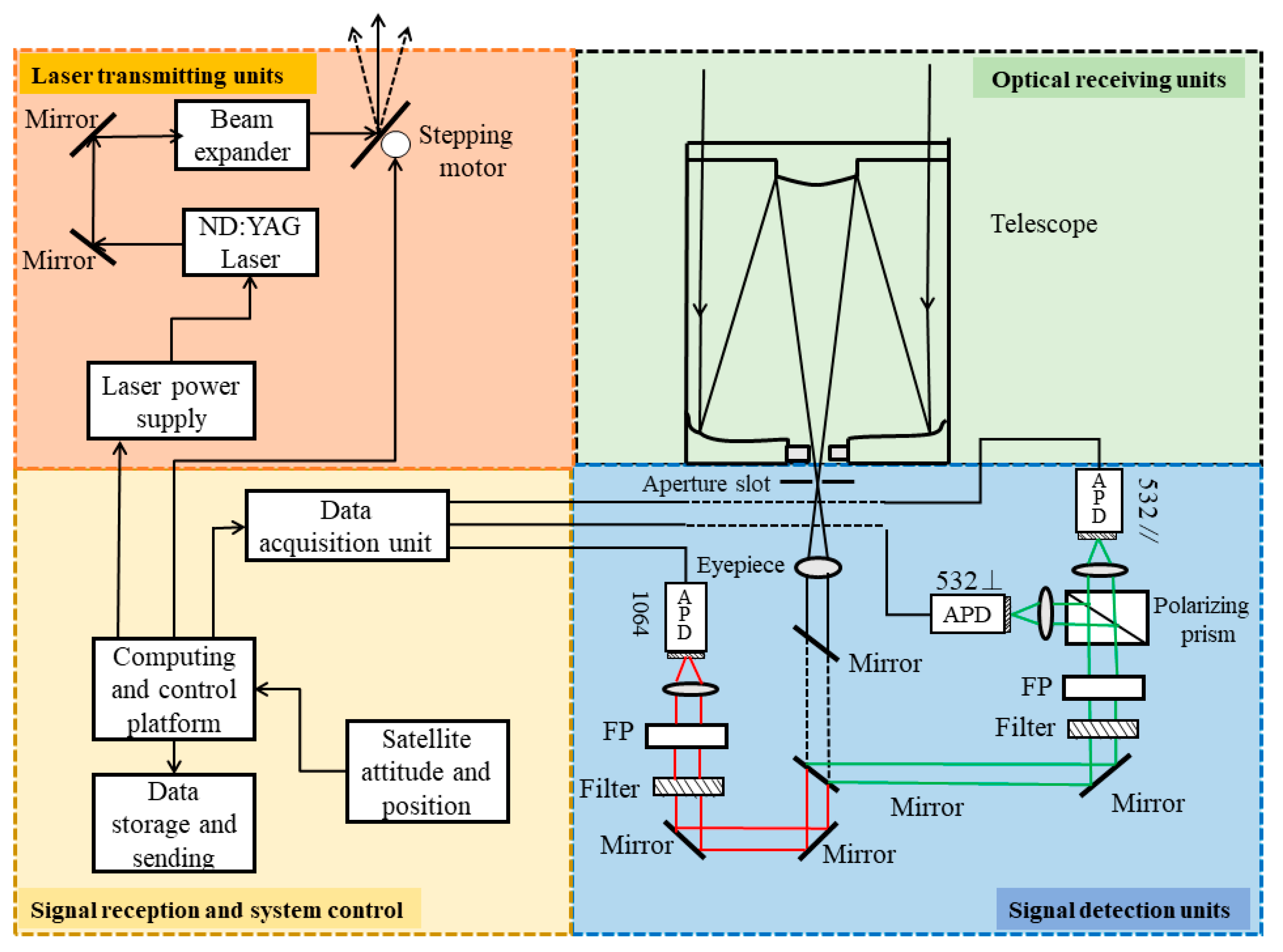
| Laser transmitting units | Single-pulse laser energy | 3 mJ@532 nm 6 mJ@1064 nm |
| Laser transmission frequency | 1000 Hz | |
| Transmission optical efficiency | 95% | |
| Optical receiving units | Telescope receiving aperture | 400 mm |
| Receiving field angle | 0.2 mrad | |
| Receiving optical efficiency | 0.4 | |
| Filter bandwidth | 0.3 nm | |
| Signal detection units | Detection efficiency | 60%@532 nm 5%@1064 nm |
| Dark count rate | 100 Hz | |
| Extinction ratio of polarizing prism | 3000:1 | |
| Data receiving units | Sampling resolution | 15 m (100 ns) |
| Sampling depth | 40,000 | |
| Satellite load units | Orbital altitude | 600 km |
| Sky background radiation | 0.2@532 nm(W·m−2·sr−1·nm−1) 0.08@1064 nm(W·m−2·sr−1·nm−1) | |
| Vertical resolution | 15 m~120 m (vertical resolution) | |
| Horizontal resolution | 1 s~10 s (7~70 km horizontal resolution) |
| Influence Categories | Influence Factors | Parameters Range | Influence Ratio | Remarks |
|---|---|---|---|---|
| System parameters | Receiving area | 0.125~0.785 (m2) | 6.3 | 0.4~1 m caliber |
| Optical transmittance | 10%~50% | 5 | -- | |
| Receiving field Angle | 0.1~0.5 (mrad) | 5 | -- | |
| Filter bandwidth | 0.01~0.3 (nm) | 30 | -- | |
| Detection efficiency | 4%~80% | 20 | -- | |
| Atmospheric parameters | Sky background radiation intensity | 0~0.2@532 nm/0.08@1064 nm (W·m−2·sr−1·nm−1) | ˃10,000 | night~day |
| Measurement parameters | Spatial resolution | 15~300 (m) | 20 | -- |
| Time resolution | 1~20 (s) | 20 | 7~150 km |
Disclaimer/Publisher’s Note: The statements, opinions and data contained in all publications are solely those of the individual author(s) and contributor(s) and not of MDPI and/or the editor(s). MDPI and/or the editor(s) disclaim responsibility for any injury to people or property resulting from any ideas, methods, instructions or products referred to in the content. |
© 2023 by the authors. Licensee MDPI, Basel, Switzerland. This article is an open access article distributed under the terms and conditions of the Creative Commons Attribution (CC BY) license (https://creativecommons.org/licenses/by/4.0/).
Share and Cite
Ji, J.; Xie, C.; Xing, K.; Wang, B.; Chen, J.; Cheng, L.; Deng, X. Simulation of Compact Spaceborne Lidar with High-Repetition-Rate Laser for Cloud and Aerosol Detection under Different Atmospheric Conditions. Remote Sens. 2023, 15, 3046. https://doi.org/10.3390/rs15123046
Ji J, Xie C, Xing K, Wang B, Chen J, Cheng L, Deng X. Simulation of Compact Spaceborne Lidar with High-Repetition-Rate Laser for Cloud and Aerosol Detection under Different Atmospheric Conditions. Remote Sensing. 2023; 15(12):3046. https://doi.org/10.3390/rs15123046
Chicago/Turabian StyleJi, Jie, Chenbo Xie, Kunming Xing, Bangxin Wang, Jianfeng Chen, Liangliang Cheng, and Xu Deng. 2023. "Simulation of Compact Spaceborne Lidar with High-Repetition-Rate Laser for Cloud and Aerosol Detection under Different Atmospheric Conditions" Remote Sensing 15, no. 12: 3046. https://doi.org/10.3390/rs15123046