Weather Radar Echo Extrapolation with Dynamic Weight Loss

Abstract

Precipitation nowcasting is an important tool for economic and social services, especially for forecasting severe weather. The crucial and challenging part of radar echo image prediction is the focus of radar-based precipitation nowcasting. Recently, a number of deep learning models have been designed to solve the problem of extrapolating radar images. Although these methods can generate better results than traditional extrapolation methods, the issue of error accumulation in precipitation forecasting is exacerbated by using only the mean square error (MSE) and mean absolute error (MAE) as loss functions. In this paper, we approach the problem from the perspective of the loss function and propose dynamic weight loss (DWL), a simple but effective loss function for radar echo extrapolation. The method adds model self-adjusted dynamic weights to the weighted loss function and structural similarity index measures. Radar echo extrapolation experiments are performed on four models, ConvLSTM, ConvGRU, PredRNN, and PredRNN++. Radar reflectivity is predicted using Nanjing University C-band Polarimetric (NJU-CPOL) weather radar data. The quantitative statistics show that using the DWL method reduces the MAE of the four models by up to 10.61%, 5.31%, 14.8%, and 13.63%, respectively, over a 1 h prediction period. The results show that the DWL approach is effective in reducing the accumulation of errors over time, improving the predictive performance of currently popular deep learning models.

1. Introduction

The forecast of precipitation intensity within 2 h is known as precipitation nowcasting [1]. The primary technique used in the 0–2 h proximity forecasting technique is radar echo extrapolation, even though forecasts are often only accurate for up to 1 h [2]. Radar echo extrapolation is vital for localized weather warnings, offering prompt and accurate weather notifications for travel, agriculture, tourism, and daily life. However, it is difficult to anticipate the distribution of short-duration precipitation in a specific area due to the intrinsic complexity and non-linear characteristic of short-duration precipitation systems [3].

The main techniques for extrapolating radar images are the single centroid method, the cross-correlation method (such as Tracking Radar Echoes by Correlation, TREC), and the optical flow method [4,5,6]. The single centroid method is a memory 3D radar tracking technique that enables extrapolation by identifying and following convective single-body characteristics of radar echoes, such as volume and reflectivity factor center of weight, and computing their center-of-mass, volume, and other characteristics [7]. The single centroid method is mainly used for the identification, tracking, and analysis of thunderstorms and can effectively identify precipitation cloud masses to predict the location of thunderstorm cloud masses [8]. It is mainly suitable for tracking and short-term forecasting of strong convective storms. However, the method has limited ability to predict large-scale precipitation echoes and is less effective for single overlapping echoes and for short-term forecasting of large-scale or multiple cloud masses precipitation systems. That is, the single centroid method is superior in stable precipitation forecasting and less effective when local convection changes are rapid [9,10]. The cross-correlation method calculates the maximum correlation of precipitation echoes in different spaces within a short period of time to obtain information on the motion vectors of the echoes. The time interval of the precipitation echoes should be short because the deformation of the precipitation echoes will scramble the motion vectors [11]. The TREC algorithm is simple and easy to implement and is more suitable for slowly changing weather processes. However, for sudden strong convective weather, there are often some biases and low data utilization, which affect the final forecast [12,13]. The optical flow is essentially a vector of motion of all pixel points in the two-dimensional projected image of the target. Compared to the single centroid and cross-correlation methods, the optical flow method is more likely to capture fast-moving and small-scale convective clouds and is based on the change of grey image level at different moments, based on the calculation of the rate of change of the pixel of each pixel point in the adjacent moments to obtain the optical flow solution [14]. The method is based on the change of pixels in the image in the time domain and the correlation between adjacent frames to determine the correspondence between the previous frame and the current frame, thus calculating the motion information of the object between the adjacent frames [15,16,17]. Subsequently, forecasters have optimized and upgraded the optical flow method and achieved good results in practical operational forecasting. However, it relies on the principle of linear extrapolation, which assumes no deformation of the radar echoes over a short period of time. Therefore, there is still some error in fast-moving and changing echoes [18].

In recent years, deep learning has been used in many fields, including target detection, semantic segmentation, and image recognition. They all have in common the construction of models to learn from large amounts of data to fit a non-linear system. For this reason, the use of large amounts of weather radar data for short-range forecasting is attracting the attention of many researchers. The deep learning approach treats the problem of short-range precipitation forecasting as a time series forecasting problem, which is the process of predicting the values of spatial and temporal variables based on historical time series data [19]. Similarly, the objective of precipitation proximity forecasting is to use previously observed radar echo sequences to predict echo images, with image time intervals of approximately 6 min and distribution of each pixel value between 0 and 70. In this work, two-dimensional radar echo images are predicted for each point in time, and the measured values are the radar reflectivity. Thus, the observed data at any moment in time can be represented by a tensor: $x_t\in R^{P\times W\times H}$, where R denotes the domain of the observed features, P denotes the measured value over time, and W and H denote the width and height of the state tensor and the input tensor, respectively [20]. The time series prediction problem can thus be described as:

$${\tilde{x}}_{t+1},\cdots ,{\tilde{x}}_{t+L}=\underset{t+1,\cdots ,t+L}{\arg \max p}(x_{t+1},\cdots ,x_{t+L}|{\widehat{x}}_{t-k+1},\cdots ,{\widehat{x}}_t)$$

(1)

The formula can be interpreted as using observations of historical length K, including current observations $({\widehat{x}}_{t-k+1},\cdots ,{\widehat{x}}_t)$, to predict future series of length L $({\tilde{x}}_{t+1},\cdots ,{\tilde{x}}_{t+L})$ and to approximate the true series $(x_{t+1},\cdots ,x_{t+L})$ as closely as possible.

Spatiotemporal sequence prediction involves two aspects: spatial correlation and temporal dynamics [21]. The performance of a prediction system depends on its ability to remember the relevant structure information. Currently, there are two main categories of neural network models for spatiotemporal sequence prediction: one is based on convolutional neural network (CNN) structures for sequence image generation, and the other is based on recurrent neural networks (RNN) for sequence image prediction [22]. Long Short-Term Memory (LSTM) networks, gated recurrent units (GRU), and RNN can all be used often in the processing of time series [23,24,25]. In 2015, a team at the Hong Kong University of Science and Technology combined LSTM with CNNs for the first time to propose the ConvLSTM model [26]. The model replaces the Hadamard product in a fully connected LSTM with a convolution operation, improving the model’s ability to learn spatial information rather than just temporal information. However, the introduction of the convolution kernel leads to spatial position invariance, which is a drawback for weather patterns with rotation and deformation. In 2017, the team further improved the ConvLSTM by proposing the Trajectory Gate Recurrent Unit (TrajGRU) model [27]. This model adds a certain degree of distortion resistance compared to the previous model, but the effect in practice is not very different from that of ConvLSTM. In the same year, Wang et al. proposed a model with a sawtooth connection structure spatiotemporal LSTM (ST-LSTM), which can transmit memory states horizontally and vertically between layers [28]. By introducing temporal and spatial memory units, shape deformation and motion trajectories can be modeled efficiently. However, ST-LSTM faces the problem of gradient disappearance. To solve this problem, in 2018, the team proposed the PredRNN++ model, an upgraded version of PredRNN, to capture long-term memory dependence by introducing the gradient highway unit module [29]. The model has two main improvements: a new Casual LSTM, which adds more non-linear operations and facilitates the capture of short-term dynamic changes, and a Gradient Highway Unit (GHU), a structure that makes it easier to retain gradients when back-propagating and solves the problem of gradient disappearance. The above networks were used in hand-written digit prediction, precipitation prediction, traffic prediction, and human behavior prediction [30,31,32,33].

Previous research has increased the complexity of network structures and recursive units to increase the precision of radar echo extrapolation. Although the performance of these models for radar echo extrapolation has improved, the number of model parameters, memory usage, and training time have all increased significantly. Additionally, how these forecasting algorithms calculate losses is too single and does not account for the error characteristics of the prediction results, which limits the prediction performance of the models. Some studies have used mean square error (MSE) or mean absolute error (MAE) to train the models. The MSE loss function aims to accommodate uncertainty in prediction by fuzzy prediction, taking the average of the possible outputs. This is because the average of all possible outcomes will result in an overall minimum in the parameter space during training. Similarly, the MAE loss predicts the median of all such outcomes, which can result in reduced resolution and loss of image detail [34,35]. Therefore, based on the current study, it was found that in radar echo extrapolation, the difficulty of predicting the latter frames of the forecast time in different training stages of the model increases gradually as the model training time goes backward, resulting in a serious long-term error accumulation phenomenon [36]. This is because there are problems with how losses are calculated in some studies, which average out the weights of all predicted images. Previous works have mainly enhanced the learning capability of deep learning models by improving model structures. For example, PredRNN [28] and PredRNN++ [29] have enhanced the ability of deep learning models to capture complex weather changes by proposing more complex recurrent units. However, their approach adds a large number of model parameters and intermediate variables, which significantly increases the time and memory cost of training. These methods often have limited improvement in such complex precipitation forecasting scenarios as they do not take into account the nature of the forecast results of existing models. Therefore, this study proposes a dynamic weight loss (DWL) method assigned to each frame for radar precipitation prediction. The general idea is to design a dynamic weight for each frame based on the prediction results of current spatiotemporal sequence forecasting models, then calculate the loss for each frame, and finally sum up each loss. Considering that the output results of the model change dynamically during the training process, we do not set each weight to a fixed value and let the model learn to self-assign the weights. Therefore, the method can adaptively assign weights according to the change in prediction difficulty in each frame, thus improving the performance of existing spatiotemporal sequence prediction models. The main contributions of this paper can be summarized as follows:

(1)

It is found that the prediction difficulty of each radar echo image in the spatiotemporal sequence prediction task is different at different training stages and that the error of the images gradually increases as the prediction time increases. Severe error accumulation leads to increasingly inaccurate extrapolation of results at a later stage. The existing MSE and MAE loss functions calculate the error directly for all images and have the same penalty weight for each prediction echo frame, so the model increasingly does not focus on the hard-to-predict images, which is a problem with how loss is calculated in the current study.

(2)

This study proposes a DWL method assigned to each frame. The error weights are calculated for each frame based on the model forecast results. Then, the losses are calculated for each frame, and finally, all losses are summed. We design a DWL function for radar precipitation forecasting, such that the level of attention given by the model to each frame changes dynamically and is determined by the model.

(3)

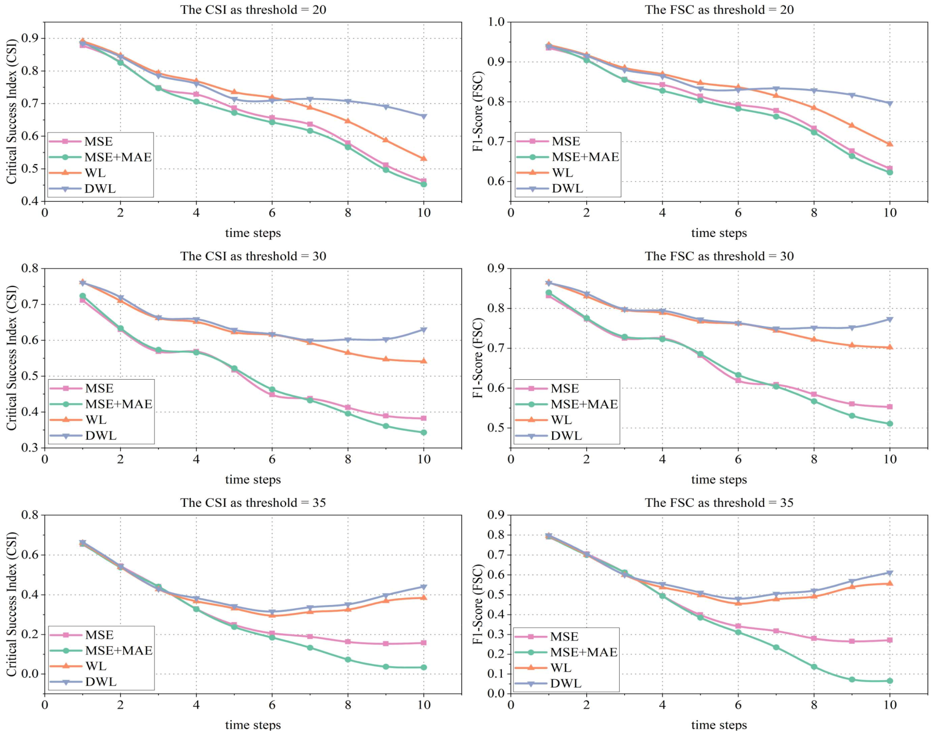
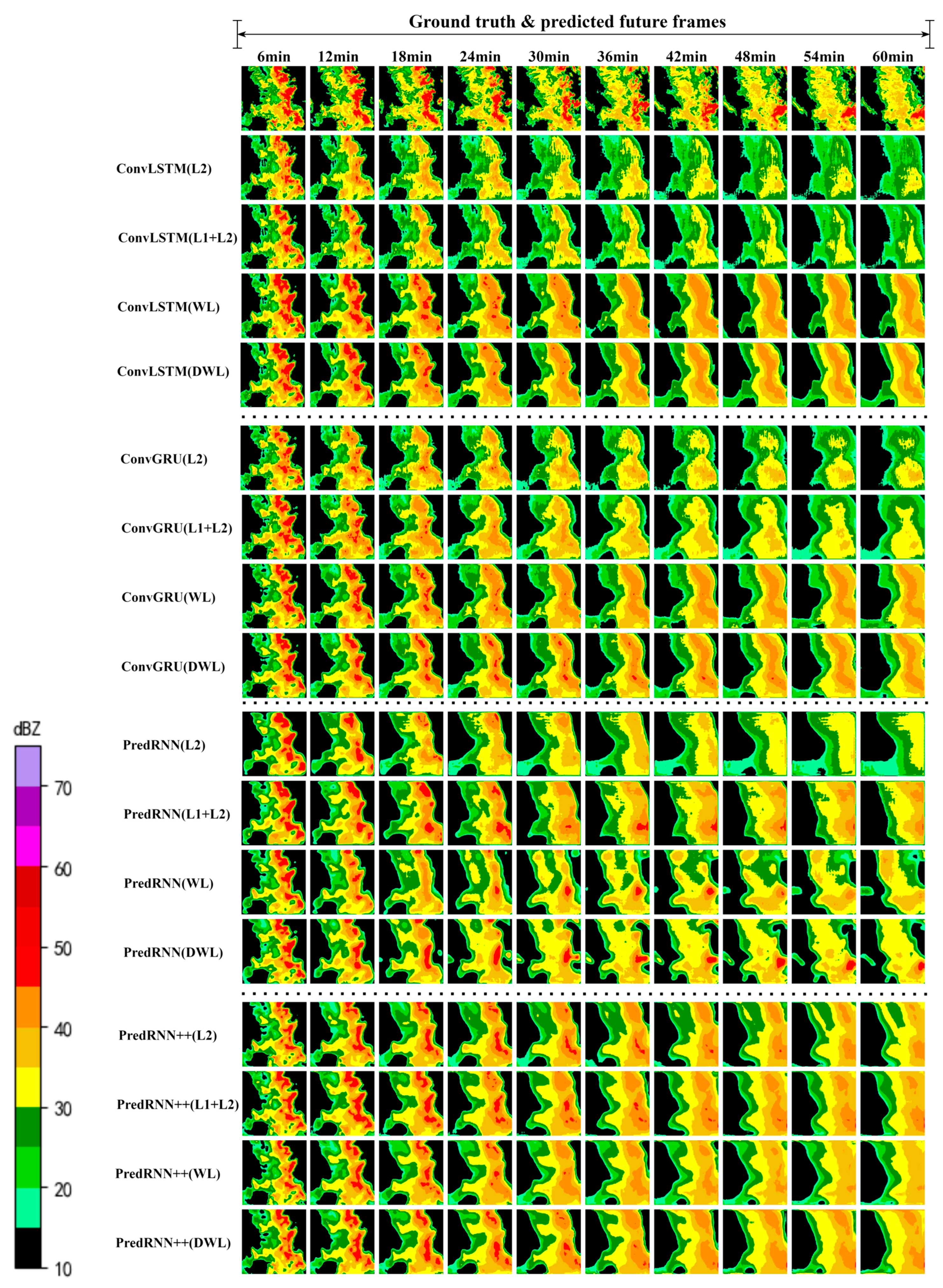
The Nanjing University C-band Polarimetric (NJU-CPOL) dataset is used to validate the method proposed in this study. The experimental results show that the proposed DWL method performs better compared to other loss methods, improves the performance of the ConvLSTM, ConvGRU, PredRNN and PredRNN++ models, and alleviates the error accumulation problem of radar precipitation forecasting to some extent.

2. Materials

In this section, the radar echo prediction data used are first introduced, and the radar data pre-processing is described. Then, a brief review of the algorithms used in this study for radar precipitation prediction is presented.

2.1. Weather Radar Dataset

The radar echo data for this study are from C-band dual polarimetric weather radar data operated by Nanjing University (NJU-CPOL). The data time span is from 2014 to 2019 and includes 268 precipitation events. The radar data are scanned over an area of 256 × 256 km with a 3 km contour, values ranging from 0–70 and radar scan intervals of approximately 6–7 min.

Due to the large size of the original images and GPU memory limitations, it is not conducive to conducting experiments, so each echo image is cropped from 256 × 256 to a 128 × 128 region. It is observed that not all of the data contained precipitation events and that the probability of precipitation events is low. Including these samples in the dataset would affect the training results, so some events with no or weak precipitation are removed.

For each folder of radar echo data, the continuous images are sliced into disjoint subsets using a 15-frame wide sliding window. Thus, each sequence consists of 15 frames, using the first 5 frames for input and the next 10 frames for prediction. That is, each sequence consists of 30 min of observations as input and the successive 60 min of observations as output. A total of 9330 samples are obtained from the training set and 1860 samples from the validation set. Samples outside the training and validation sets are selected to test the generalization ability of the model. There is no temporal overlap between the samples. All data is linearly normalized to obtain values between zero and one before being fed into the model.

2.2. Deep Learning Model

2.2.1. ConvLSTM

The ConvLSTM proposed by Shi et al. [26] is an improvement of LSTM. Compared to the Fully Connected LSTM, ConvLSTM uses convolution operation in input-to-state and state-to-state transfer, and this operation can extract spatial features efficiently. The model in this study forms an encoded prediction structure by stacking multiple ConvLSTM cells equally. This method has proven to be effective in dealing with spatiotemporal sequence prediction problems. The ConvLSTM cells mainly consist of the input gate $i_t$, forget gate $f_t$, storage cell $C_t$, a hidden state $H_t$, and output gate $O_t$, as represented in Equation (2).

$$\begin{array}{c}{i}_t=\sigma (W_{xi}\ast X_t+W_{hi}\ast H_{t-1}+W_{ci}\circ C_{t-1}+b_i)\hfill \\ f_t=\sigma (W_{xf}\ast X_t+W_{hf}\ast H_{t-1}+W_{cf}\circ C_{t-1}+b_f)\hfill \\ C_t=f_t\circ C_{t-1}+i_t\circ \tanh (W_{xc}\ast X_t+W_{hc}\ast H_{t-1}+b_c)\hfill \\ O_t=\sigma (W_{xo}\ast X_t+W_{ho}\ast H_{t-1}+W_{co}\circ C_t+b_o)\hfill \\ H_t=O_t\circ \tanh (C_t)\hfill \end{array}$$

(2)

where ‘$\ast$’ and ‘$\circ$’ denote the convolution operation and Hadamard product, respectively, σ denotes the sigmoid activation function, and b indicates bias.

2.2.2. ConvGRU

ConvGRU is a further improvement on ConvLSTM by Shi et al. [27]. Compared with ConvLSTM, ConvGRU has fewer parameters, effectively avoiding the gradient vanishing problem and retaining the basic gating mechanism. Similarly, the fully connected operation in GRU is replaced by a convolution operation, which has the ability to capture spatiotemporal correlations. The ConvGRU unit mainly consists of an update gate $Z_t$, reset gate $R_t$, and hidden state $H_t$, as represented in Equation (3).

$$\begin{array}{c}{Z}_t=\sigma (W_{xz}\ast X_t+W_{hz}\ast H_{t-1}+b_z)\hfill \\ R_t=\sigma (W_{xr}\ast X_t+W_{hr}\ast H_{t-1}+b_r)\hfill \\ H_t^{\prime }=\tanh (W_{xh}\ast X_t+R_t\circ (W_{hh}\ast H_{t-1})+b_h)\hfill \\ H_t=(1-Z_t)\circ H_t^{\prime }+Z_t\circ H_{t-1}\hfill \end{array}$$

(3)

where ‘$\ast$’ and ‘$\circ$’ denote the convolution operation and Hadamard product, respectively, σ and tanh denote the activation functions, $X_t$ denotes the input to the model, and b indicates bias.

2.2.3. PredRNN

PredRNN was proposed by Wang et al. [28]. The study pointed out that both temporal and spatial information is important, and in previous studies, the bottom layer would ignore the top layer information in the previous time step. To better model spatial correlation and temporal dynamics, a new Spatiotemporal LSTM (ST-LSTM) unit is proposed in PredRNN, which can extract and remember both spatial and temporal information. The ST-LSTM contains standard Temporal Memory and Spatiotemporal Memory, where the standard Temporal Memory is the same as the LSTM and the second part is the new Spatiotemporal memory state M, which can be specifically expressed as Equation (4).

$$\begin{array}{c}{g}_t^{\prime }=\tanh (W_{xg}^{\prime }\ast X_t+W_{mg}\ast M_t^{l-1}+b_g^{\prime })\hfill \\ i_t^{\prime }=\sigma (W_{xi}^{\prime }\ast X_t+W_{mi}\ast M_t^{l-1}+b_i^{\prime })\hfill \\ f_t^{\prime }=\sigma (W_{xf}^{\prime }\ast X_t+W_{mf}\ast M_t^{l-1}+b_f^{\prime })\hfill \\ M_t^l=f_t^{\prime }\odot M_t^{l-1}+i_t^{\prime }\odot g_t^{\prime }\hfill \\ o_t=\sigma (W_{xo}\ast X_t+W_{ho}\ast H_{t-1}^l+W_{co}\ast C_t^l+W_{mo}\ast M_t^l+b_o)\hfill \\ H_t^l=o_t\odot \tanh (W_{1\times 1}\ast \left[C_t^l,M_t^l\right]\hfill \end{array}$$

(4)

where ‘$\ast$’ and ‘$\odot$’ denote convolution and element-wise multiplication, respectively. $W_{1\times 1}$ denotes a 1 × 1 convolution filter, $\sigma$ represents the sigmoid function, and b indicates bias.

2.2.4. PredRNN++

As the number of model layers increases and the prediction time lengthens, the PredRNN model suffers from gradient disappearance. To solve this problem, Wang et al. [29] proposed the PredRNN++ model. Compared to the PredRNN model, a new Casual LSTM unit and GHU were proposed. The structure can obtain stronger spatial correlation and short-term dynamic modeling capability, effectively alleviating the problem of gradient disappearance. Casual LSTM and GHU are shown in Equations (5) and (6), respectively.

$$\begin{array}{l}\left(\begin{array}{l}{g}_t\\ i_t\\ f_t\end{array}\right)=\left(\begin{array}{l}\tanh \\ \sigma \\ \sigma \end{array}\right)W_1\ast [X_t,H_{t-1}^k,C_{t-1}^k]\\ C_t^k=f_t\odot C_{t-1}^k+i_t\odot g_t\\ \left(\begin{array}{l}{g}_t^{\prime }\\ i_t^{\prime }\\ f_t^{\prime }\end{array}\right)=\left(\begin{array}{l}\tanh \\ \sigma \\ \sigma \end{array}\right)W_2\ast [X_t,C_t^k,M_t^{k-1}]\\ M_t^k=f_t^{\prime }\odot \tanh (W_3\ast M_t^{k-1})+i_t^{\prime }\odot g_t^{\prime }\\ o_t=\tanh (W_4\ast [X_t,C_t^k,M_t^k])\\ H_t^k=o_t\odot \tanh (W_5\ast [C_t^k,M_t^k])\end{array}$$

(5)

$$\begin{array}{l}{P}_t=\tanh (W_{px}\ast X_t+W_{pz}\ast Z_{t-1})\\ S_t=\sigma (W_{sx}\ast X_t+W_{sz}\ast Z_{t-1})\\ Z_t=S_t\odot P_t+(1-S_t)\odot Z_{t-1}\end{array}$$

(6)

In the above equations, ‘$\ast$’ and ‘$\odot$’ denote convolution and element-wise multiplication, respectively, round brackets denote systems of equations, and square brackets denote concatenation of the tensors. $W_{1\sim 5}$ is the convolution filter, and $\sigma$ is the sigmoid function.

3. Proposed Method

This section first describes the problem of MSE and MAE loss functions used in previous radar precipitation studies. Then, the proposed dynamic weights constructed from radar precipitation prediction results are presented. Next, this study combines the weighted combined loss function with dynamic weights to propose the DWL method.

3.1. MSE and MAE Loss

In time series prediction, a radar echo sequence of length k can be expressed as $\left\{y_1,y_2,\cdots ,y_k\right\}$. The absolute error at any moment can be expressed as $\Delta e_i=\left|{\widehat{y}}_i-y_i\right|$ (where ${\widehat{y}}_i$ and $y_i$ represent the predicted and observed echo images at the ith moment, respectively) so that the MSE (L2 Loss) and MAE (L1 Loss) can be described as in Equation (7).

$$MSE+MAE=\frac{1}{k}\left({\displaystyle \sum _{i=1}^k\left(\Delta e_i^2+\Delta e_i\right)}\right)$$

(7)

From the equation, it can be seen that the weight of each predicted image loss is the same and equal to 1. Therefore, as the model makes iterative predictions, the error becomes progressively larger as the prediction timescale increases, which leads to more inaccurate predictions. The direct calculation of MSE and MAE for all images limits the model’s performance, which is consistent with most current work on radar echo extrapolation. In order to cope with all conditional situations, the MSE loss function aims to accommodate the uncertainty in prediction by fuzzy prediction or taking the mean of all possible outputs. This averaging of all possible outcomes results in the smallest overall value in the parameter space during training. The MAE loss is the median of all outcomes predicted. Other loss functions based on L-parameters can also lead to reduced resolution of the prediction results (e.g., artifacts and low-quality results) [37,38].

It is known from previous studies that the difficulty of each prediction frame is different because the RNN model adds the prediction result of the previous frame when predicting the next frame. This type of extrapolation model predicts the next frame, conditional on the outcome of the previous frame. The error of each subsequent frame gradually accumulates over time, leading to a loss of image accuracy, which is extremely unfavorable for spatiotemporal sequence prediction. Therefore, this direct calculation of MSE or MAE loss is not ideal.

3.2. Dynamic Weight

The larger the error of the image, the greater the prediction difficulty of the image. For this reason, this study uses the error of the image to indicate its prediction difficulty. Assuming that m future frames are predicted, as expressed in Equation (8), with values ranging from zero to one, a larger value indicates a larger proportion of the total loss, meaning that the image is more difficult to predict.

$$d_i=\frac{\Delta e_i}{\Delta e_1+\Delta e_2+\cdots +\Delta e_m}(i=1:m)$$

(8)

where $d_i$ is the prediction difficulty of an image at any moment.

In the spatiotemporal sequence prediction task, the prediction difficulty is different for each frame. For each task, due to differences in the temporal dimension, the loss calculated for each image is considered when assigning a weight to the frame. We find that the difficulty of each task also varies dynamically during the different training phases of the model. Therefore, we cannot average the loss weights of all tasks as in previous work, which would cause the model to penalize tasks of different difficulty equally, nor can we assign fixed weights to each image and thus fail to arrive at more accurate prediction results. Therefore, this proposed method introduces a dynamic weighting approach to alleviate the error accumulation problem.

The prediction difficulty of an image at different moments is determined by the current model’s prediction results. For this reason, the loss weights are dynamically adjusted for each frame. The more difficult a task is, the more corresponding loss weights it receives, i.e., the more strongly the model penalizes it, and vice versa. Suppose a sequence of length m is predicted so that for any moment, the loss weights can be expressed as in Equation (9).

$$w_i=k{(d_i+b)}^x=k{(\frac{\Delta e_i}{\Delta e_1+\Delta e_2+\cdots +\Delta e_m}+b)}^x$$

(9)

where k, b, and x are hyperparameters, k = b = 1; b is a bias to prevent the possibility of a weight of 0; and the index x is set to 2.

3.3. Dynamic Weight Loss

The model requires not only a scheme for the rational allocation of weights to each task but also a superior loss function. In several radar echo image prediction studies, MSE or MAE was often used directly as the loss function, resulting in a loss of all predicted mean and echo details and poor image quality. Ambiguous extrapolation results also lead to an underestimation of the strength of the radar echoes and a lack of small-scale detail in the echoes, which makes it difficult for the model to forecast strong convective systems.

Using the NJU-CPOL radar echo dataset, the distribution of the radar reflectivity values is analyzed. Six sets of strong echo samples are randomly selected from all samples. Each set contained 10 consecutive frames of echo images, and the radar reflectivity thresholds were set at 30 and 40. These were used to divide the values into three ranges for numerical statistics, with each range accounting for approximately the values shown in Figure 1. The importance of predicting the intensity and location of strong echoes cannot be overstated, as there is a large proportion of values for echoes that are less likely linked to strong precipitation and a small proportion of values that are highly likely related to strong precipitation. Therefore, loss functions with unbalanced weights are needed.

Higher reflectivity is given greater weight, which means that the model further focuses on areas that are highly susceptible to meteorological hazards. Then, the MSE and MAE with weights can be expressed as Equations (10) and (11), respectively.

$$B-MSE(R,\widehat{R})={\displaystyle \sum _{t,h,w}weigh{t}_{t,h,w}}\ast {(R_{t,h,w}-{\widehat{R}}_{t,h,w})}^2$$

(10)

$$B-MAE(R,\widehat{R})={\displaystyle \sum _{t,h,w}weigh{t}_{t,h,w}}\ast \left|R_{t,h,w}-{\widehat{R}}_{t,h,w}\right|$$

(11)

where $weigh{t}_{t,h,w}=\left\{\begin{array}{l}0.5\hspace{1em}\hspace{1em}0\le R_{t,h,w}<5\\ 1.0\hspace{1em}\hspace{1em}5\le R_{t,h,w}<10\\ 2.0\hspace{1em}\hspace{1em}10\le R_{t,h,w}<20\\ 5.0\hspace{1em}\hspace{1em}20\le R_{t,h,w}<30\\ 10.0\hspace{1em} 30\le R_{t,h,w}<40\\ 20.0\hspace{1em} R_{t,h,w}\ge 40\end{array}\right\}$; $R_{t,h,w}$ and ${\widehat{R}}_{t,h,w}$ denote the label reflectivity and predicted reflectivity at coordinates (t, h, and w), respectively, and $weigh{t}_{t,h,w}$ denotes the weight at coordinates (t, h, and w).

In order to improve the detail and resolution of the radar echo images, we add the loss function: $L_{ssim}=1-ssim$, where SSIM is the structural similarity index measure, which can be expressed as Equation (12):

$$SSIM=\frac{(2{\mu }_Y{\mu }_{\overline{Y}}+C_1)(2{\sigma }_{Y\overline{Y}}+C_2)}{({\mu }_Y^2+{\mu }_{\overline{Y}}^2+C_1)({\sigma }_Y^2+{\sigma }_{\overline{Y}}^2+C_2)}$$

(12)

where ${\mu }_Y$ and ${\mu }_{\overline{Y}}$ denotes the mean of the true and predicted values, respectively, estimating the brightness of the image, ${\sigma }_{Y\overline{Y}}$ denotes the covariance between the true and predicted values, measuring the structural similarity of the image, ${\sigma }_Y$ and ${\sigma }_{\overline{Y}}$ denotes the variance between the true and predicted values, respectively, and estimating the contrast of the image, and $C_1$ and $C_2$ are two constants to avoid dividing by zero.

In summary, this study proposes a weighted loss function. The specific representation is shown in Equation (13), where, $\beta$ and $\gamma$ are the reduction and amplification coefficients, respectively, used to adjust the difference in values between the two loss functions, $\beta =5\times {10}^{-4}$, $\gamma =1\times {10}^4$, and $\widehat{y}$ and $y$ denote the predicted and observed images, respectively.

$$WL(\widehat{y},y)=\beta (B-MSE+B-MAE)+\gamma L_{ssim}$$

(13)

Combined with the dynamic weights $w_i$ proposed in this study, the DWL can be expressed as Equation (14), where $w_i$ and $W{L}_i$ denote the dynamic weights and losses at the ith frame, respectively, and ${\widehat{y}}_i$ and $y_i$ denote the predicted and observed images at the ith frame, respectively.

$$DWL={\displaystyle \sum _{i=1}^m(w_i\ast W{L}_i})={\displaystyle \sum _{i=1}^m\left[{(\frac{\Delta e_i}{\Delta e_1+\Delta e_2+\cdots +\Delta e_m}+1)}^2\ast WL({\widehat{y}}_i,y_i)\right]}$$

(14)

4. Experiment

In this section, the experimental setup is first described. Then, the evaluation indicators used in this study are detailed. Finally, the experimental results and the analysis of the results are presented.

4.1. Experimental Setup

In order to verify the validity of the proposed method, the experimental setup is as follows: four sets of experiments are prepared, each using a different loss function, including MSE (L2), MSE + MAE (L1 + L2), WL, and DWL. For the same model, the experiments are set up identically, except using different loss functions.

The experiments are conducted using the Adam optimizer, with an initial learning rate of 0.0001. Using the learning rate auto-decay method, the learning rate decays by 0.1 after every 5 epochs when the loss value does not decrease, as shown in Equation (15), where the factor is the learning rate reduction factor. Here, the factor is set to 0.1. The iteration batch size during training is set to five. All models and algorithms are implemented on the Pytorch framework and run on the NVIDIA GeForce RTX 2080ti.

$$\mathrm{LearningRate}=\mathrm{factor}\ast \mathrm{LearningRate}$$

(15)

4.2. Evaluation Metrics

To test the ability of the four loss function methods to predict radar reflectivity over a range of magnitudes, two common meteorological precipitation evaluation metrics are used: the Critical Success Index (CSI), which is defined as the summed average of the precision, and the F1-Score balanced F Score (FSC) which combines the results of both precision and recall, with FSC values ranging from zero to one. Values closer to 1 indicate better model performance, and closer to zero indicate worse model performance. Assuming that there are two categories, positive and negative, denoted by one and zero, respectively, a confusion matrix is constructed, as shown in

Table 1. Confusion matrix for classification.

	Predicted Yes	Predicted No
Observed Yes	TP (true positive)	FN (false negative)
Observed No	FP (false positive)	TN (true negative)

.

The CSI and FSC indicators can be expressed as Equations (16) and (19), and the Precision and Recall indicators can be expressed as Equations (17) and (18).

$$\mathrm{CSI}=\frac{\mathrm{TP}}{\mathrm{TP}+\mathrm{FP}+\mathrm{FN}}$$

(16)

$$\mathrm{Precision}=\frac{\mathrm{TP}}{\mathrm{TP}+\mathrm{FP}}$$

(17)

$$\mathrm{Recall}=\frac{\mathrm{TP}}{\mathrm{TP}+\mathrm{FN}}$$

(18)

$$\mathrm{F}1\text{-}\mathrm{Score}=2\ast \frac{\mathrm{Precision}\ast \mathrm{Recall}}{\mathrm{Precision}+\mathrm{Recall}}$$

(19)

The CSI and FSC metrics can directly reflect the strengths and weaknesses of the model, with larger CSI and FSC values indicating better model performance. Based on the above evaluation metrics, we set three different thresholds of 20 dBZ, 30 dBZ, and 35 dBZ to test the prediction results. In addition, this study also uses MAE to evaluate the model performance, with lower MAE values indicating a lower error, which is calculated as shown in Equation (20), where $y_i$ and ${\widehat{y}}_i$ represent the observed and predicted data, respectively.

$$\mathrm{MAE}=\frac{1}{\mathrm{k}}{\displaystyle \sum _{\mathrm{i}=1}^{\mathrm{k}}\left|{\mathrm{y}}_{\mathrm{i}}-{\widehat{\mathrm{y}}}_{\mathrm{i}}\right|}$$

(20)

4.3. Experimental Results

In order to analyze the advantages of DWL for the model in terms of long-term forecasting, this study compares and analyzes CSI, FSC, and MAE of four groups of experiments. The results are shown in

Table 2. Comparative results of the ConvLSTM model using different loss methods for CSI, FSC, and MAE.

ConvLSTM	CSI↑			FSC↑			MAE↓
Threshold	20	30	35	20	30	35
MSE	0.6713	0.5065	0.3084	0.7965	0.6661	0.4478	5.759
MSE + MAE	0.6613	0.5016	0.2665	0.7886	0.6600	0.3806	5.645
WL	0.7206	0.6270	0.4015	0.8331	0.7686	0.5650	5.616
DWL	0.7475	0.6485	0.4209	0.8539	0.7856	0.5856	5.148

,

Table 3. Comparative results of the ConvGRU model using different loss methods for CSI, FSC, and MAE.

ConvGRU	CSI↑			FSC↑			MAE↓
Threshold	20	30	35	20	30	35
MSE	0.6886	0.5774	0.3722	0.8107	0.7273	0.5279	5.881
MSE + MAE	0.6259	0.5279	0.3357	0.7588	0.6806	0.4822	5.930
WL	0.7233	0.6345	0.4435	0.8368	0.7749	0.6088	5.781
DWL	0.7238	0.6424	0.4457	0.8374	0.7813	0.6108	5.569

,

Table 4. Comparative results of the PredRNN model using different loss methods for CSI, FSC, and MAE.

PredRNN	CSI↑			FSC↑			MAE↓
Threshold	20	30	35	20	30	35
MSE	0.6400	0.5727	0.3872	0.7731	0.7203	0.5400	5.899
MSE + MAE	0.6697	0.5734	0.3918	0.7971	0.7232	0.5452	5.657
WL	0.7121	0.6636	0.4620	0.8296	0.7975	0.6270	5.240
DWL	0.7293	0.6653	0.4655	0.8416	0.7987	0.6321	5.026

and

Table 5. Comparative results of the PredRNN++ model using different loss methods for CSI, FSC, and MAE.

PredRNN++	CSI↑			FSC↑			MAE↓
Threshold	20	30	35	20	30	35
MSE	0.6919	0.6496	0.4824	0.8118	0.7856	0.6464	5.811
MSE + MAE	0.7254	0.6664	0.5022	0.8369	0.7986	0.6652	5.497
WL	0.7244	0.6730	0.5123	0.8369	0.8040	0.6739	5.241
DWL	0.7276	0.6909	0.5232	0.8383	0.8165	0.6843	5.019

, with “↑” indicating higher indicator scores and “↓” indicating lower indicator scores.

For the ConvLSTM model (Table 2), WL loss improves in all metrics compared to MSE or MSE + MAE, but the DWL method performs best. For the threshold of 35 dBZ, the improvement in CSI (FSC) compared to the other three methods is 0.1125, 0.1544, and 0.0194 (0.1378, 0.2050, and 0.0206), an improvement of 36.48%, 57.94%, and 4.83% (30.77%, 53.86%, and 3.65%), respectively. The MAE shows a decrease of 0.611, 0.497, and 0.468 compared to the other three methods.

As shown in Table 3, the CSI and FSC indicators for the ConvGRU model perform more similarly and DWL performs slightly better at 30 dBZ. The DWL method performs better at 20 and 35 dBZ. For the threshold of 20 dBZ, the DWL method improves the CSI by 0.0352, 0.0979, and 0.0005 (5.11%, 15.64%, and 0.07%), respectively. The FSC improves by 0.0267, 0.0786, and 0.0006 (3.29%, 10.36%, and 0.07%), respectively. The MAE decreases by 0.312, 0.361, and 0.212, respectively.

For the PredRNN model (Table 4), the DWL method outperforms the other methods in all three metrics, with the MSE method performing the worst. With a threshold of 30 dBZ, the improvement in the CSI compared to the MSE, MSE + MAE, and WL methods is 0.0926, 0.0919, and 0.0017 (16.17%, 16.03%, and 0.26%), respectively. The FSC metric shows an improvement of 0.0784, 0.0755, and 0.0012 (10.88%, 10.44%, and 0.15%), respectively, and MAE shows a decrease of 0.873, 0.631, and 0.214, respectively.

For the PredRNN++ model (Table 5), the MSE method performs the worst, while the DWL method outperforms the other loss methods and shows the best performance. With a threshold of 35 dBZ, the improvement in CSI metrics compared to the other loss methods is 0.0408, 0.0210, and 0.0109 (8.46%, 4.18%, and 2.13%), respectively, while the FSC shows an improvement of 0.0379, 0.0191, and 0.0104 (5.86%, 2.87%, and 1.54%), respectively. The MAE shows decreases of 0.792, 0.478, and 0.222, respectively.

To visualize the change process of each evaluation indicator more clearly, CSI and FSC curves are plotted for all predicted time points (Figure 2, Figure 3, Figure 4 and Figure 5).

From Figure 2, it can be observed that MSE and MSE + MAE show a significant drop in performance as the prediction timescale increases. The longer the prediction time, the larger the drop. In contrast, the WL and DWL methods show a slow decline in performance, especially at thresholds of 30 dBZ and 35 dBZ, where they remain at higher performance levels in the later stages. The CSI and FSC for the DWL method improve by 5.14% and 3.15%, respectively, at time point 10 compared to time point 7 when the threshold is 30 dBZ, and by 39.45% and 27.40% at time point 10 compared to time point 6, respectively, when the threshold is 35 dBZ. The DWL method proposed in this study improves the metrics more significantly. Firstly, the B-MSE and B-MAE in the DWL method provide a larger weight to the high-value reflectivity, which improves the prediction accuracy in the high-value echo region, and the improvement is more obvious for higher reflectivity values. Furthermore, the ConvLSTM model does not capture spatiotemporal correlations effectively, and its predictions tend to be increasingly inaccurate. Based on the inaccurate prediction results produced by the model, our method adds dynamic weights to the inaccurate radar images, i.e., the DWL method assigns greater weights to the later radar images. This leads to a small improvement in some of the later metrics, but the overall trend in performance is downward.

From Figure 3, the CSI and FSC for all methods show a decreasing trend throughout the prediction time, with the MSE and MSE + MAE methods showing the most significant decline after the sixth time point, while the WL and DWL methods remain at high levels after the seventh time point. From Figure 4, overall, the CSI and FSC for all methods show a decreasing trend, and the decline becomes progressively larger in the later stages, with the DWL method performing the best and the decline in performance reducing in the later stages. As shown in Figure 5, all metrics show a decreasing trend, with MSE and MSE + MAE performance decreasing most significantly, reflecting the fact that the loss function is not good at long-term forecasting. Combining the prediction results of the four models, the ConvGRU model performs the worst, while the PredRNN++ model is more accurate, with the images retaining more detail.

In summary, this research method improves the prediction performance of existing deep learning models and effectively mitigates the problem of long-term error accumulation in radar images, demonstrating the effectiveness of the loss method design.

Figure 6 shows the MAE of ConvLSTM, ConvGRU, PredRNN, and PredRNN++ using different loss methods trend over the 10 prediction time points. In general, errors gradually increase with prediction time for all models and loss methods. It is noted that the increase in the error of the first three methods becomes larger in the middle and late stages of prediction. In contrast, the DWL method slows down the accumulation of errors in the middle and late stages of the prediction and remains at a better level, effectively suppressing the deteriorating forecast performance.

Firstly, the MAEs of all four models show an increasing trend, mainly due to the recursive structure of this class of extrapolation models, which must depend on the previous frame to predict the next frame, which leads to a gradual accumulation of image errors. Secondly, the MSE and MAE methods show more significant error accumulation, mainly because these two loss functions average out the loss weights for each frame. Finally, the DWL method is more advantageous because it assigns different weights to different frames.

To better compare and understand the results, we visualize two prediction cases for all models and loss methods. Case 1 is characterized by a gradual weakening of the echoes and a large change in the overall echo pattern. Case 2 is characterized by a gradual reduction in the area of strong echoes without a large change in the overall pattern of the echoes. The visualization results of these two cases are shown in Figure 7 and Figure 8, respectively, which visually compare the prediction results of different models using different loss methods, with darker colors indicating stronger possible precipitation intensity.

As shown in Figure 7 and Figure 8, the results of all models and methods show a weakening of intensity, which is closely related to the structure of the models themselves. Among them, in ConvLSTM and ConvGRU, which were first proposed for spatiotemporal sequence prediction, the stacked structure does not easily learn the intensity changes of the echoes, leading to increasingly inaccurate prediction results. The PredRNN and PredRNN++ models also produce inaccurate predictions but have improved performance compared to the first two models, as they predict clearer images and retain more details. The overall shape of the later echoes is closer to the actual situation. In comparing all the loss methods, the MSE and MSE + MAE methods perform the worst, and the images become increasingly blurred and fade as the prediction time gets longer. In contrast, the other two methods retain more high-value echo areas, and the images are clearer and closer to the real situation because the B-MSE and B-MAE enhance the focus on high-value areas. Furthermore, the addition of SSIM improves the quality of the predicted echo images. In particular, the DWL method is more advantageous. From the visualization results, we can find that the dynamic weights improve the accuracy of the later images and even outperform some of the earlier ones, which indicates that the method acts as a guide to the model, instructing it to learn some tasks with greater errors.

5. Conclusions

In this study, we address the issue where the MSE loss or MAE loss used by current mainstream time series prediction models can exacerbate the accumulation of errors in long-term precipitation forecasts, resulting in increasingly inaccurate predicted radar images. We analyze the error characteristics of model prediction results from the perspective of the loss function used by current models and propose the DWL method assigned to each frame. The DWL allows the model to actively focus on those images that are more difficult to predict based on the change in difficulty of the model forecast for each frame.

The proposed method is thoroughly tested against four deep-learning models using the NJU-CPOL radar echo dataset. The DWL shows good results in improving the performance of a normal RNN model to a certain extent without introducing additional training overhead. The experimental results show that the DWL outperforms current commonly used loss methods and can improve the forecasting performance of current radar echo extrapolation models. Therefore, the experimental results validate its effectiveness.

The advantage of our proposed method is that it does not increase the model’s training time consumption and memory. In addition, DWL is a simple but effective loss function. The disadvantage of the method is that there is still some discrepancy between the prediction results and the actual observations, which cannot be compensated by the model and the loss function. Furthermore, we should also address the problem from the perspective of data factors. In future work, we should also consider data-level influences. In practical terms, precipitation is a complex microphysical process influenced by various environmental factors, such as humidity, temperature, and topography. It is not reasonable to consider only a single radar variable without taking into account the variability of other meteorological elements. Studies have shown that the distribution characteristics of the dual-polarization radar variables, including specific differential phase (K_dp) and differential reflectivity (Z_dr), contain hydrometeorological and microphysical information on the developmental changes of strong convection, and they have important research value for radar echo extrapolation tasks [39,40]. Therefore, it is not reasonable for existing models to learn only the spatiotemporal variability of the radar reflectivity characteristics. The use of dual-polarization radar data containing multiple variables for strong convection forecasting merits continued research.

References

1. Agrawal, S.; Barrington, L.; Bromberg, C.; Burge, J.; Gazen, C.; Hickey, J. Machine Learning for Precipitation Nowcasting from Radar Images. arXiv 2019, arXiv:191212132. [Google Scholar] [CrossRef]
2. Ehsani, M.R.; Zarei, A.; Gupta, H.V.; Barnard, K.; Behrangi, A. Nowcasting-Nets: Deep Neural Network Structures for Precipitation Nowcasting Using IMERG. arXiv 2021, arXiv:210806868. [Google Scholar] [CrossRef]
3. Sun, J.; Xue, M.; Wilson, J.W.; Zawadzki, I.; Ballard, S.P.; Onvlee-Hooimeyer, J.; Joe, P.; Barker, D.M.; Li, P.-W.; Golding, B.; et al. Use of NWP for Nowcasting Convective Precipitation: Recent Progress and Challenges. Bull. Am. Meteorol. Soc. 2014, 95, 409–426. [Google Scholar] [CrossRef] [Green Version]
4. Woo, W.; Wong, W. Operational Application of Optical Flow Techniques to Radar-Based Rainfall Nowcasting. Atmosphere 2017, 8, 48. [Google Scholar] [CrossRef] [Green Version]
5. Johnson, J.T.; Mackeen, P.L.; Witt, A.; Mitchell, E.D.W.; Stumpf, G.J.; Eilts, M.D.; Thomas, K.W. The Storm Cell Identification and Tracking Algorithm: An Enhanced WSR-88D Algorithm. Weather Forecast. 1998, 13, 263–276. [Google Scholar] [CrossRef]
6. Rinehart, R.; Garvey, E. Three-Dimensional Storm Motion Detection by Conventional Weather Radar. Nature 1978, 273, 287–289. [Google Scholar] [CrossRef]
7. Fang, W.; Zhang, F.; Sheng, V.S.; Ding, Y. SCENT: A New Precipitation Nowcasting Method Based on Sparse Correspondence and Deep Neural Network. Neurocomputing 2021, 448, 10–20. [Google Scholar] [CrossRef]
8. Crane, R.K. Automatic Cell Detection and Tracking. IEEE Trans. Geosci. Electron. 1979, 17, 250–262. [Google Scholar] [CrossRef]
9. Dixon, M.; Wiener, G. TITAN: Thunderstorm Identification, Tracking, Analysis, and Nowcasting—A Radar-Based Methodology. J. Atmos. Ocean. Technol. 1993, 10, 785–797. [Google Scholar] [CrossRef]
10. Lanpher, A. Evaluation of the Storm Cell Identification and Tracking Algorithm Used by the WSR-88D. Ph.D. Thesis, Cornell University, Ithaca, NY, USA, 2012. [Google Scholar]
11. Laroche, S.; Zawadzki, I. Retrievals of Horizontal Winds from Single-Doppler Clear-Air Data by Methods of Cross Correlation and Variational Analysis. J. Atmos. Ocean. Technol. 1995, 12, 721. [Google Scholar] [CrossRef]
12. Zou, H.; Wu, S.; Shan, J.; Yi, X. A Method of Radar Echo Extrapolation Based on TREC and Barnes Filter. J. Atmos. Ocean. Technol. 2019, 36, 1713–1727. [Google Scholar] [CrossRef]
13. Li, P.W.; Lai, E. Short-Range Quantitative Precipitation Forecasting in Hong Kong. J. Hydrol. 2004, 288, 189–209. [Google Scholar] [CrossRef]
14. Bowler, N.E.; Pierce, C.E.; Seed, A. Development of a Precipitation Nowcasting Algorithm Based upon Optical Flow Techniques. J. Hydrol. 2004, 288, 74–91. [Google Scholar] [CrossRef]
15. Dosovitskiy, A.; Fischer, P.; Ilg, E.; Hausser, P.; Hazirbas, C.; Golkov, V.; Van Der Smagt, P.; Cremers, D.; Brox, T. Flownet: Learning Optical Flow with Convolutional Networks. In Proceedings of the IEEE International Conference on Computer Vision, Santiago, Chile, 13–16 December 2015; pp. 2758–2766. [Google Scholar]
16. Ayzel, G.; Heistermann, M.; Winterrath, T. Optical Flow Models as an Open Benchmark for Radar-Based Precipitation Nowcasting (Rainymotion v0. 1). Geosci. Model Dev. 2019, 12, 1387–1402. [Google Scholar] [CrossRef] [Green Version]
17. Marrocu, M.; Massidda, L. Performance Comparison between Deep Learning and Optical Flow-Based Techniques for Nowcast Precipitation from Radar Images. Forecasting 2020, 2, 194–210. [Google Scholar] [CrossRef]
18. Liu, Y.; Xi, D.-G.; Li, Z.-L.; Hong, Y. A New Methodology for Pixel-Quantitative Precipitation Nowcasting Using a Pyramid Lucas Kanade Optical Flow Approach. J. Hydrol. 2015, 529, 354–364. [Google Scholar] [CrossRef]
19. Hu, Y.; Chen, L.; Wang, Z.; Pan, X.; Li, H. Towards a More Realistic and Detailed Deep-Learning-Based Radar Echo Extrapolation Method. Remote Sens. 2021, 14, 24. [Google Scholar] [CrossRef]
20. Jing, J.; Li, Q.; Ding, X.; Sun, N.; Tang, R.; Cai, Y. AENN: A Generative Adversarial Neural Network for Weather Radar Echo Extrapolation. Int. Arch. Photogramm. Remote Sens. Spat. Inf. Sci. 2019, 42, 89–94. [Google Scholar] [CrossRef] [Green Version]
21. Zeng, Q.; Li, H.; Zhang, T.; He, J.; Zhang, F.; Wang, H.; Qing, Z.; Yu, Q.; Shen, B. Prediction of Radar Echo Space-Time Sequence Based on Improving TrajGRU Deep-Learning Model. Remote Sens. 2022, 14, 5042. [Google Scholar] [CrossRef]
22. Castro, R.; Souto, Y.M.; Ogasawara, E.; Porto, F.; Bezerra, E. Stconvs2s: Spatiotemporal Convolutional Sequence to Sequence Network for Weather Forecasting. Neurocomputing 2021, 426, 285–298. [Google Scholar] [CrossRef]
23. Greff, K.; Srivastava, R.K.; Koutník, J.; Steunebrink, B.R.; Schmidhuber, J. LSTM: A Search Space Odyssey. IEEE Trans. Neural Netw. Learn. Syst. 2016, 28, 2222–2232. [Google Scholar] [CrossRef] [PubMed] [Green Version]
24. Fu, R.; Zhang, Z.; Li, L. Using LSTM and GRU Neural Network Methods for Traffic Flow Prediction. In Proceedings of the 2016 31st Youth Academic Annual Conference of Chinese Association of Automation (YAC), Wuhan, China, 11–13 November 2016; pp. 324–328. [Google Scholar]
25. Qin, Y.; Song, D.; Chen, H.; Cheng, W.; Jiang, G.; Cottrell, G. A Dual-Stage Attention-Based Recurrent Neural Network for Time Series Prediction. arXiv 2017, arXiv:170402971. [Google Scholar] [CrossRef]
26. Shi, X.; Chen, Z.; Wang, H.; Yeung, D.-Y.; Wong, W.-K.; Woo, W. Convolutional LSTM Network: A Machine Learning Approach for Precipitation Nowcasting. Adv. Neural Inf. Process. Syst. 2015, 28, 802–810. [Google Scholar]
27. Shi, X.; Gao, Z.; Lausen, L.; Wang, H.; Yeung, D.-Y.; Wong, W.; Woo, W. Deep Learning for Precipitation Nowcasting: A Benchmark and a New Model. Adv. Neural Inf. Process. Syst. 2017, 30, 5617–5627. [Google Scholar]
28. Wang, Y.; Long, M.; Wang, J.; Gao, Z.; Yu, P.S. Predrnn: Recurrent Neural Networks for Predictive Learning Using Spatiotemporal Lstms. Adv. Neural Inf. Process. Syst. 2017, 30, 879–888. [Google Scholar]
29. Wang, Y.; Gao, Z.; Long, M.; Wang, J.; Philip, S.Y. Predrnn++: Towards a Resolution of the Deep-in-Time Dilemma in Spatiotemporal Predictive Learning. PMLR 2018, 80, 5123–5132. [Google Scholar]
30. Fang, W.; Pang, L.; Yi, W.; Sheng, V.S. AttEF: Convolutional LSTM Encoder-Forecaster with Attention Module for Precipitation Nowcasting. Intell. Autom. Soft Comput. 2021, 30, 453–466. [Google Scholar] [CrossRef]
31. He, W.; Xiong, T.; Wang, H.; He, J.; Ren, X.; Yan, Y.; Tan, L. Radar Echo Spatiotemporal Sequence Prediction Using an Improved Convgru Deep Learning Model. Atmosphere 2022, 13, 88. [Google Scholar] [CrossRef]
32. Liu, L.; Zhen, J.; Li, G.; Zhan, G.; He, Z.; Du, B.; Lin, L. Dynamic Spatial-Temporal Representation Learning for Traffic Flow Prediction. IEEE Trans. Intell. Transp. Syst. 2020, 22, 7169–7183. [Google Scholar] [CrossRef]
33. Ma, Z.; Zhang, H.; Liu, J. MS-RNN: A Flexible Multi-Scale Framework for Spatiotemporal Predictive Learning. arXiv 2022, arXiv:220603010. [Google Scholar] [CrossRef]
34. Mathieu, M.; Couprie, C.; LeCun, Y. Deep Multi-Scale Video Prediction beyond Mean Square Error. arXiv 2015, arXiv:151105440. [Google Scholar] [CrossRef]
35. Kim, B.; Han, M.; Shim, H.; Baek, J. A Performance Comparison of Convolutional Neural Network-Based Image Denoising Methods: The Effect of Loss Functions on Low-Dose CT Images. Med. Phys. 2019, 46, 3906–3923. [Google Scholar] [CrossRef] [PubMed]
36. Jing, J.; Li, Q.; Peng, X.; Ma, Q.; Tang, S. HPRNN: A Hierarchical Sequence Prediction Model for Long-Term Weather Radar Echo Extrapolation. In Proceedings of the ICASSP 2020—2020 IEEE International Conference on Acoustics, Speech and Signal Processing (ICASSP), Barcelona, Spain, 4–8 May 2020; pp. 4142–4146. [Google Scholar]
37. Rajkumar, S.; Malathi, G. A Comparative Analysis on Image Quality Assessment for Real Time Satellite Images. Indian J. Sci. Technol. 2016, 9, 1–11. [Google Scholar] [CrossRef]
38. Hao, S.; Li, S. A Weighted Mean Absolute Error Metric for Image Quality Assessment. In Proceedings of the 2020 IEEE International Conference on Visual Communications and Image Processing (VCIP), Macau, China, 1–4 December 2020; pp. 330–333. [Google Scholar]
39. Chen, H.; Chandrasekar, V.; Bechini, R. An Improved Dual-Polarization Radar Rainfall Algorithm (DROPS2. 0): Application in NASA IFloodS Field Campaign. J. Hydrometeorol. 2017, 18, 917–937. [Google Scholar] [CrossRef]
40. Chen, H.; Chandrasekar, V. Estimation of Light Rainfall Using Ku-Band Dual-Polarization Radar. IEEE Trans. Geosci. Remote Sens. 2015, 53, 5197–5208. [Google Scholar] [CrossRef]
Figure 1. Percentage of each range of values for multiple samples.
Remotesensing 15 03138 g001
Figure 2. Change trends in CSI and FSC for the ConvLSTM model using different loss methods.
Remotesensing 15 03138 g002
Figure 3. Change trends in CSI and FSC for the ConvGRU model using different loss methods.
Remotesensing 15 03138 g003
Figure 4. Change trends in CSI and FSC for the PredRNN model using different loss methods.
Remotesensing 15 03138 g004
Figure 5. Change trends in CSI and FSC for the PredRNN++ model using different loss methods.
Remotesensing 15 03138 g005
Figure 6. Change trends in MAE for ConvLSTM, ConvGRU, PredRNN, and PredRNN++ using different loss methods.
Remotesensing 15 03138 g006
Figure 7. Case 1 echo prediction results using the NJU-CPOL dataset. The first row represents the actual observation. The other rows indicate the prediction results of different models using different loss methods.
Remotesensing 15 03138 g007
Figure 8. Case 2 echo prediction results using the NJU-CPOL dataset. The first row represents the actual observations. The other rows indicate the prediction results of different models using different loss methods.
Remotesensing 15 03138 g008