3.2.1. 2.5-State Model
As described by Wang and Rothacher [
36], the receiver clock biases can be described by a low-order polynomial and a stochastic clock parameter. In this study, a quadratic polynomial consisting of an initial clock offset
, a frequency offset
and a frequency drift
is used to describe the deterministic part of the LEO satellite clock, while a stochastic clock offset
is used to capture the remaining stochastic clock behaviors at time point
. In the observation model (see Equations (1) and (2)), the LEO satellite clock bias can thus be expressed as follows:
where
indicates the time at the start of processing. For simplicity,
is expressed as
in the following contexts. The IF LEO satellite code bias that is contained in the estimable LEO satellite clock parameter is assumed constant over the processing period.
The one-state relative constraint, as discussed in Wang and Rothacher [
36], however, assumes a White Frequency Noise (WFN) of the clocks with the variance of the between-epoch relative constraint linearly increasing with the sampling interval. For other noise types, a two-state model, having both the stochastic clock offset (
) and a frequency offset (
) estimated and constrained, would be more appropriate. The frequency drift term
(see Equation (3)) is estimated as a constant in the deterministic clock model. This is equivalent to a three-state model with the variance of the relative constraint between frequency drifts of subsequent epochs set to zero. As such, the model introduced in this study is termed a “2.5”-state model. In a least-squares form, the relative constraints can be formulated as:
where
denotes the time derivative of
. To avoid singularity between
and
in Equation (3), a weak absolute constraint (set to zero) is additionally applied to
with a large standard deviation
, e.g., 1 m:
As a constant frequency offset
is previously estimated, the initial value
is also constrained to zero with a standard deviation
, such that:
The variance–covariance matrix for constraint Equations (6)–(9) is given as:
where
forms a diagonal matrix using the elements contained in
. At epoch
,
is set to
. The variance–covariance matrix of the relative constraints
is a function of the noise type, size, and sampling interval
. This will be explained later in this section.
Adding the clock constraints is the same as adding the following term to the normal equation matrix for the stochastic clock parameters of epoch
and
:
where
represents the a priori standard deviation of unit weight (on L1), assumed here 1 mm. Based on Equations (4)–(7), the matrix
is expressed as:
where
denotes the identity matrix with a size of 2. To improve the computational efficiency when solving using the batch least-squares adjustment, a pre-elimination and back-substitution strategy is applied for the epoch-wise clock and orbit parameters considering the relative constraints between subsequent epochs. The case for the one-state clock model [
37] is extended here to a two-state model.
As shown in van Dierendonck et al. [
38] and Krawinkel and Schön [
6], the system noise to be applied between subsequent clock parameters within a Kalman filter differs for different noise types. The Kalman filter, at the same time, can be equivalently expressed in the form of a sequential least-squares adjustment [
39] with:
where
represents all the O-C terms at epoch
, including any absolute constraints on the estimable parameters, e.g., the weak absolute constraints on the stochastic clock parameters (Equations (6) and (7)).
describes the observation model of all estimable parameters at epoch
, and the corresponding variance–covariance matrix of the observations is denoted as
. Among all the estimable parameters, the ones to be temporally updated are contained in the vector
. The estimated
at
, multiplied by the transition matrix
, are treated as pseudo-observations for these parameters at
.
denotes the variance–covariance matrix of
at
, which is a fully populated variance–covariance matrix for all the time-updated unknowns.
is the system noise for updating
from epoch
to
. In
, one distinguishes further between the clock parameters (
) and other parameters to be updated (
), e.g., the phase ambiguities. The clock parameters
contain, in our case, the three polynomial coefficients that are constrained as constants in time, and the stochastic clock offset
and frequency offset
, which need to be updated with their clock system noise
. The transition matrix
and the variance–covariance matrix for the total system noise
can thus be expressed as:
for which
and
denote the transition matrix and process noise matrix for
, respectively.
denotes the (
)-th element of the matrix for clock system noise
, where
here. As the sequential least-squares adjustment can also be formulated in the form of a batch least-squares [
40], the matrix
for the clock system noise replaces
in Equation (8). The standard deviation for the initial absolute constraint of the frequency offset, i.e.,
at
(see Equation (7)), is set to
. The clock model can thus be realized using a batch least-squares adjustment or a real-time filter based on sequential least-squares. In this study, the former case is applied for the tests presented due to the clock detrending method that will be discussed in
Section 4. It is noted that Gaussian distribution, as assumed in this study, may not perfectly describe the observation noise and the estimation errors. This should be considered in the integrity monitoring of the POD of LEO satellites.
Taking the WFN, the Flicker Frequency Noise (FFN), and the Random-Walk Frequency Noise (RWFN) for the LEO satellite clocks as examples,
Table 2 gives their slopes in terms of the Allan deviation [
41] and the elements in the variance–covariance matrix for the relative constraints (
,
and
), as well as the
(
) coefficients in
,
and
. The
coefficients are constant, where their amplitudes are related to the clock stabilities.
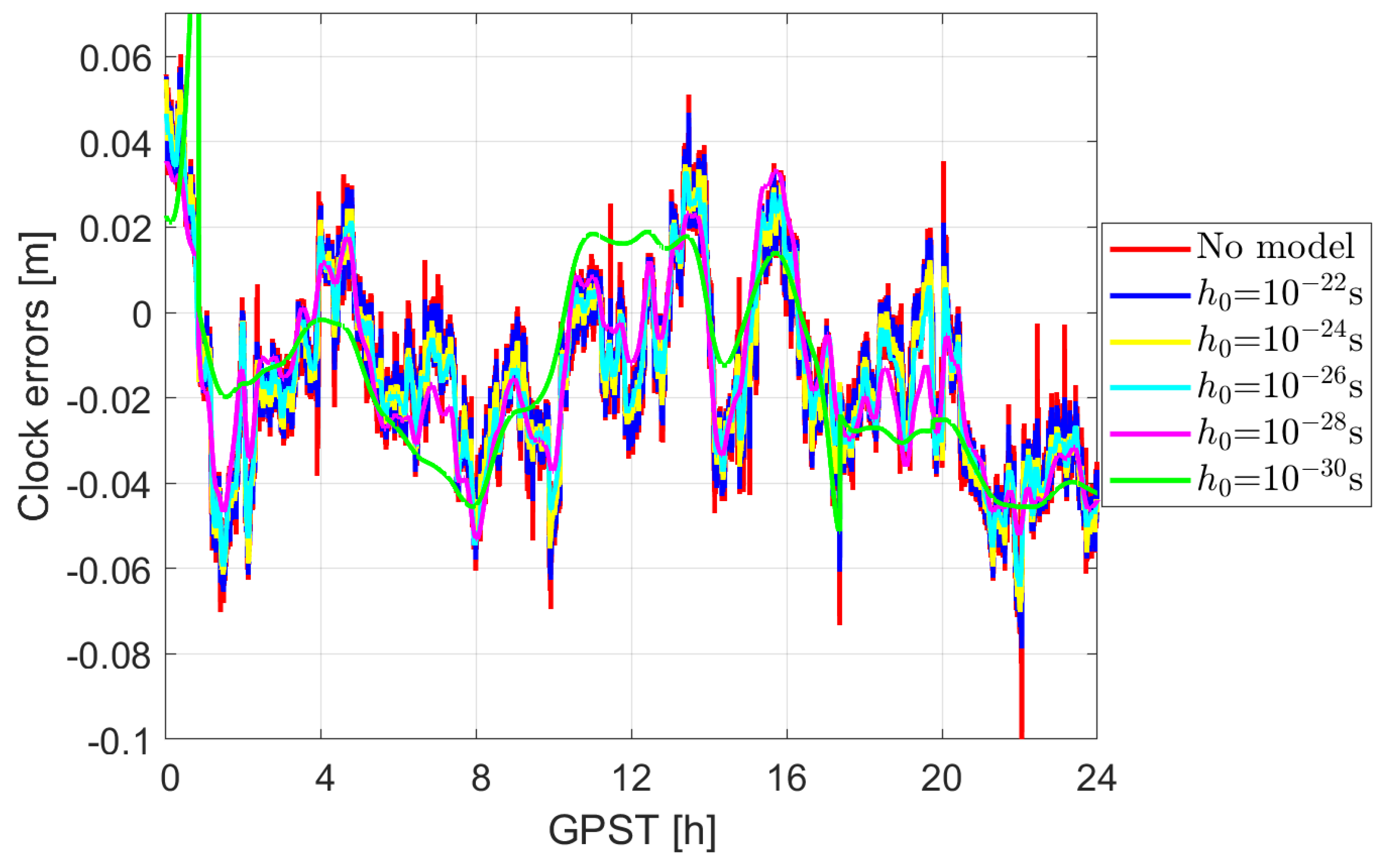
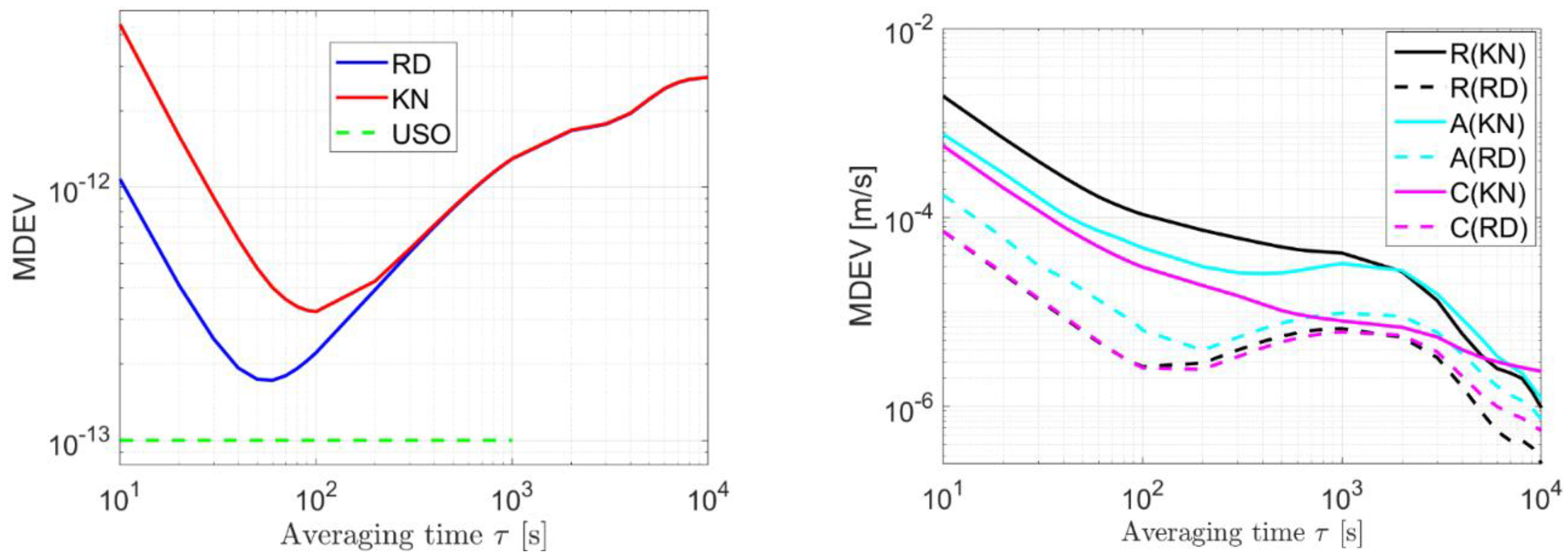
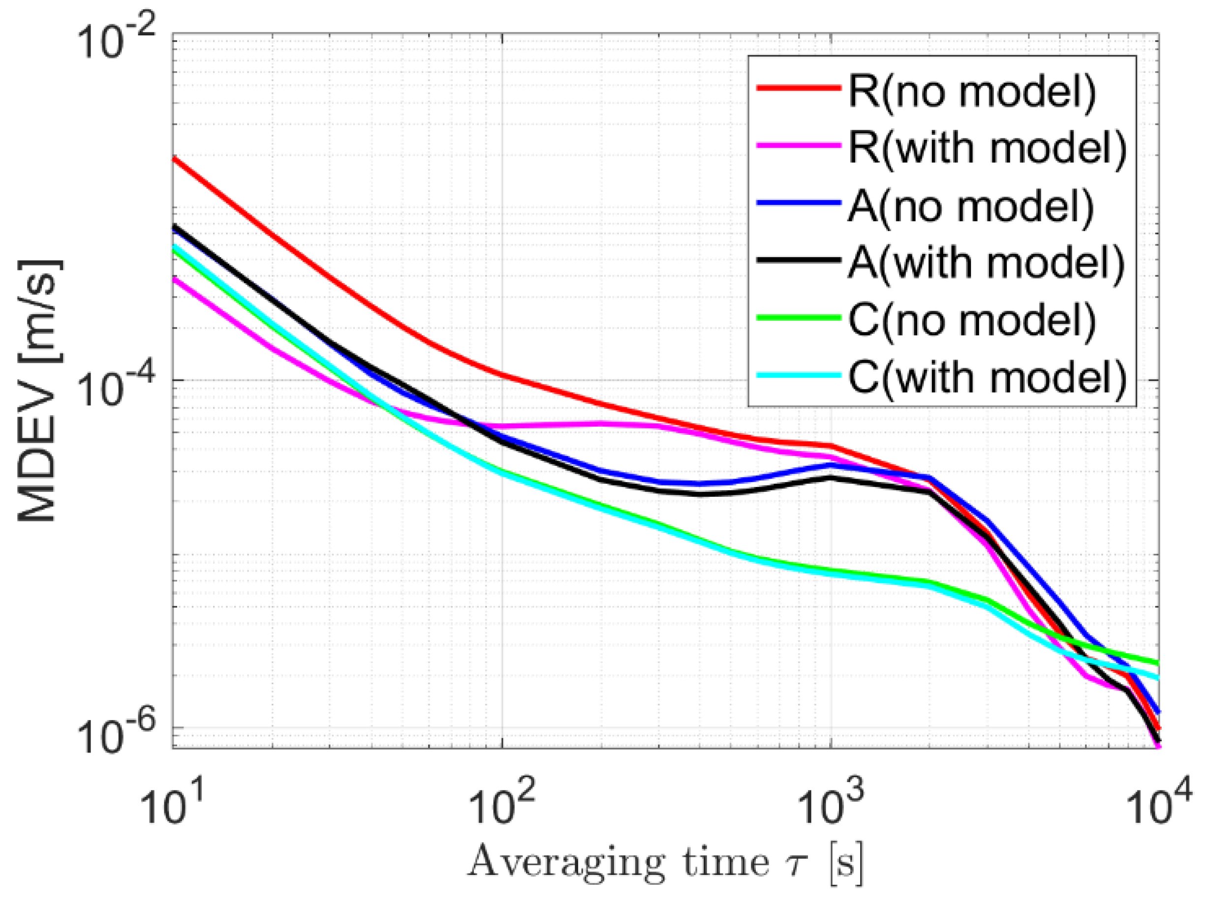
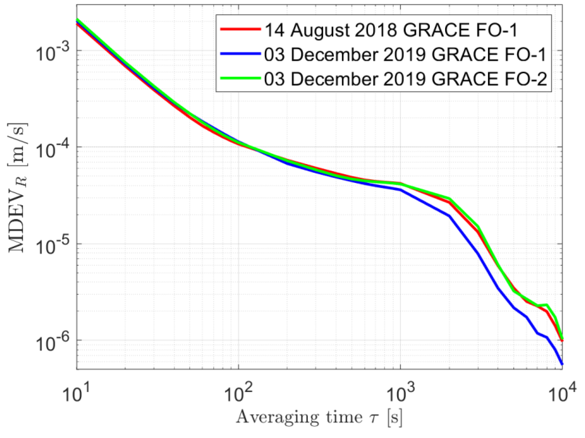
To give an example of the effects when applying the 2.5-state model of different strengths,
Figure 2 shows simulation test results for the clock errors estimated in the kinematic POD for two cases when applying and not applying the given clock model. The observation geometry of GRACE FO-1 on 14 August 2018 was used for the simulations. Only the noise and real-time GPS orbital and clock errors are considered in the O-C terms. The latter term was obtained by comparing the real-time GPS products between the French National Centre for Space Studies (CNES) [
42] and the final products from the CODE, with the clock products re-referenced to those of the final CODE products. The standard deviation of the phase and code noise is set to 0.001 m and 0.1 m, respectively. The clock model for a WFN is applied, with
(see
Figure 2) varying from
to
s. The increasing strength in the clock model directly leads to an increasing smoothing effect of the clock errors. The peak in the green line at around 00:51 and 17:22 are caused by data gaps and looser constraints. After applying the clock models, the short-term stability in the Modified Allan Deviation (MDEV) is reduced, with the reduction extended to the mid-term stability when further decreasing the
value.
3.2.2. Piece-Wise Linear Model
The PWL model estimates the clocks with linear polynomials of a pre-defined time interval
[
15]. It can be expressed as follows:
where
and
denote the clock bias at the knot point in the PWL model before and after
, respectively.
is the time interval from the knot point before
to the epoch
. The estimable parameters are clocks at a series of knot points separated by
. The determined factor of the PWL model is the time interval
.
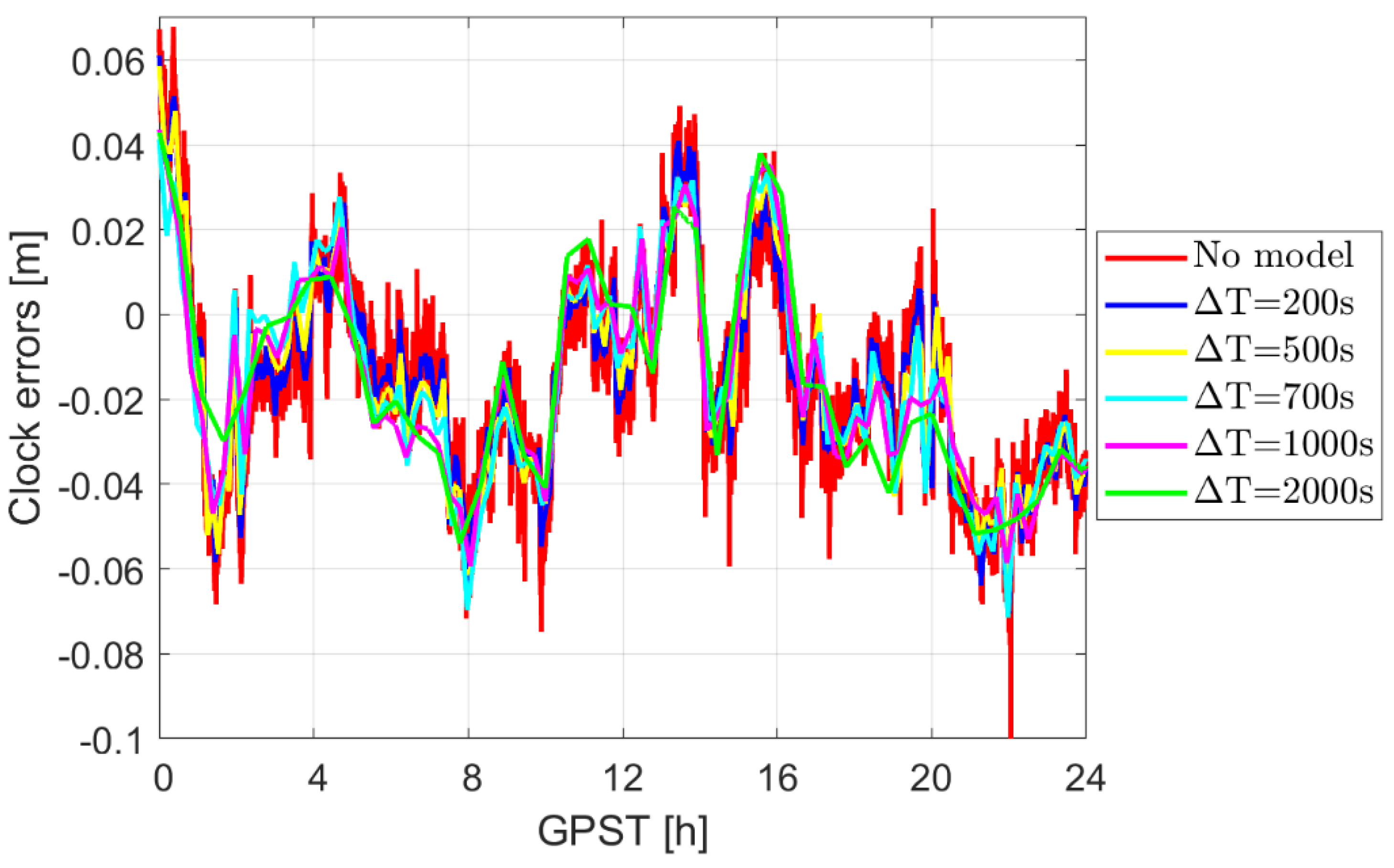
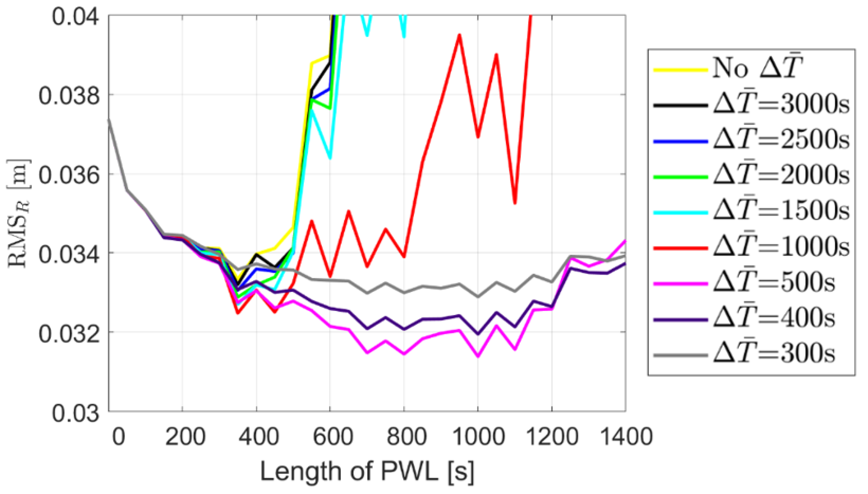
Using the same satellite geometry as in
Section 3.2.1 and considering the same noise and mis-modeled effects,
Figure 3 illustrates the smoothing effect in the kinematic clock estimates, applying the PWL model of different lengths. It can be observed that an increasing PWL length corresponds to a reduced
-value in the 2.5-state model as shown in
Figure 2. Unlike the 2.5-state model that constrains the clocks, also weakly in the long term, the PWL model puts infinitely strong constraints on clocks (above the linear polynomial) within each pre-defined
. Applying the PWL model reduces the short-term stability of the estimated clock errors by adding an infinitely strong constraint for each PWL interval, i.e., estimated as linear polynomials.
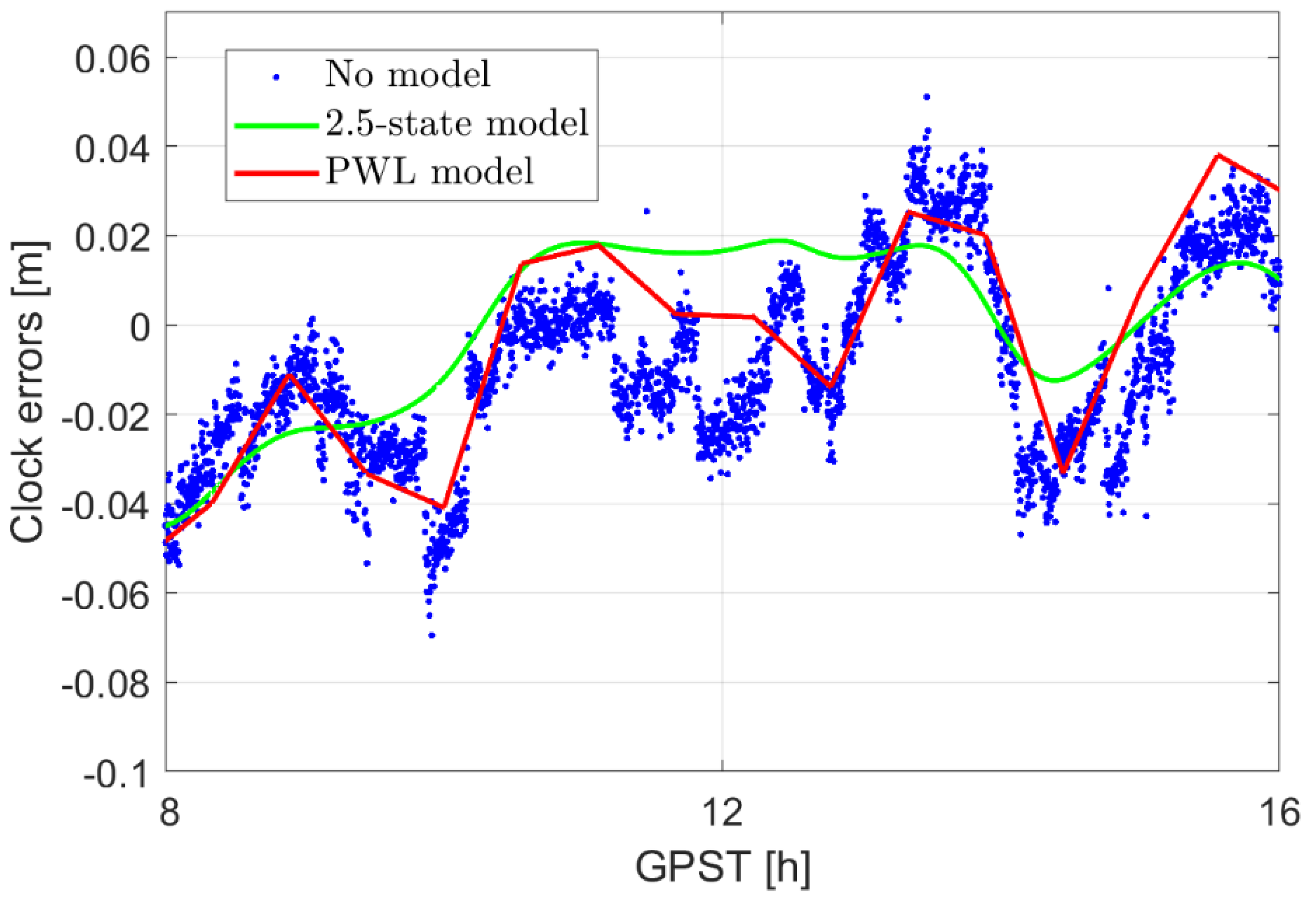
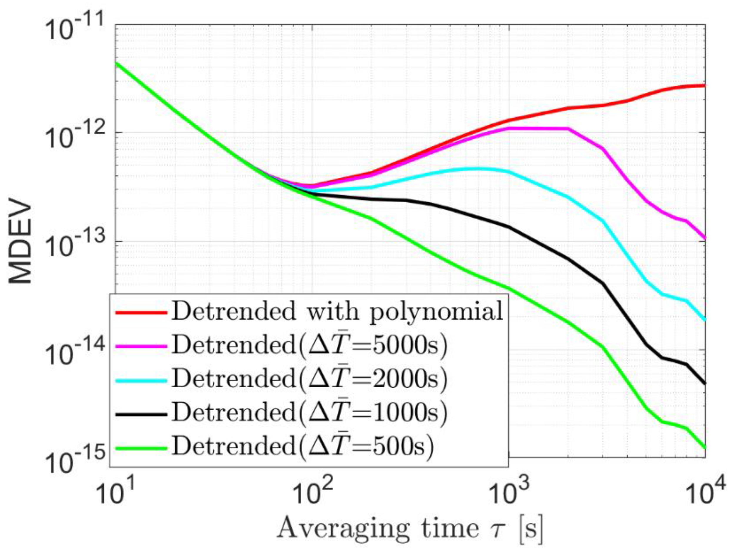
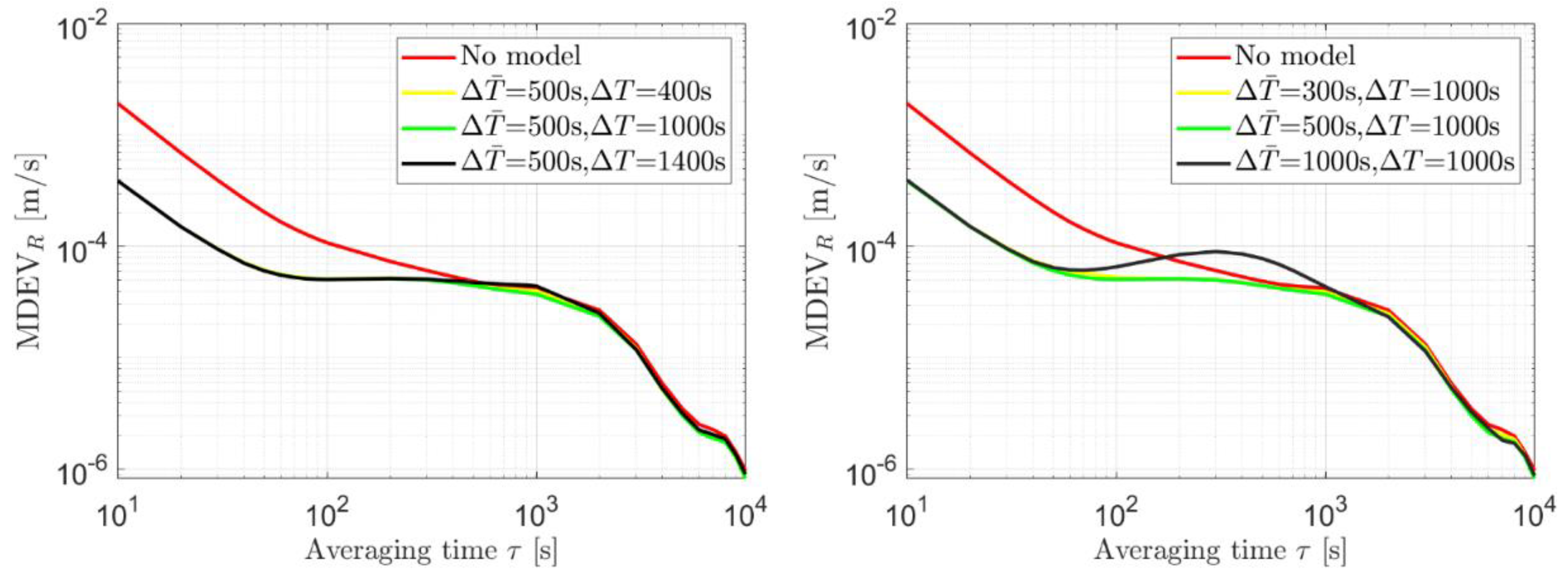
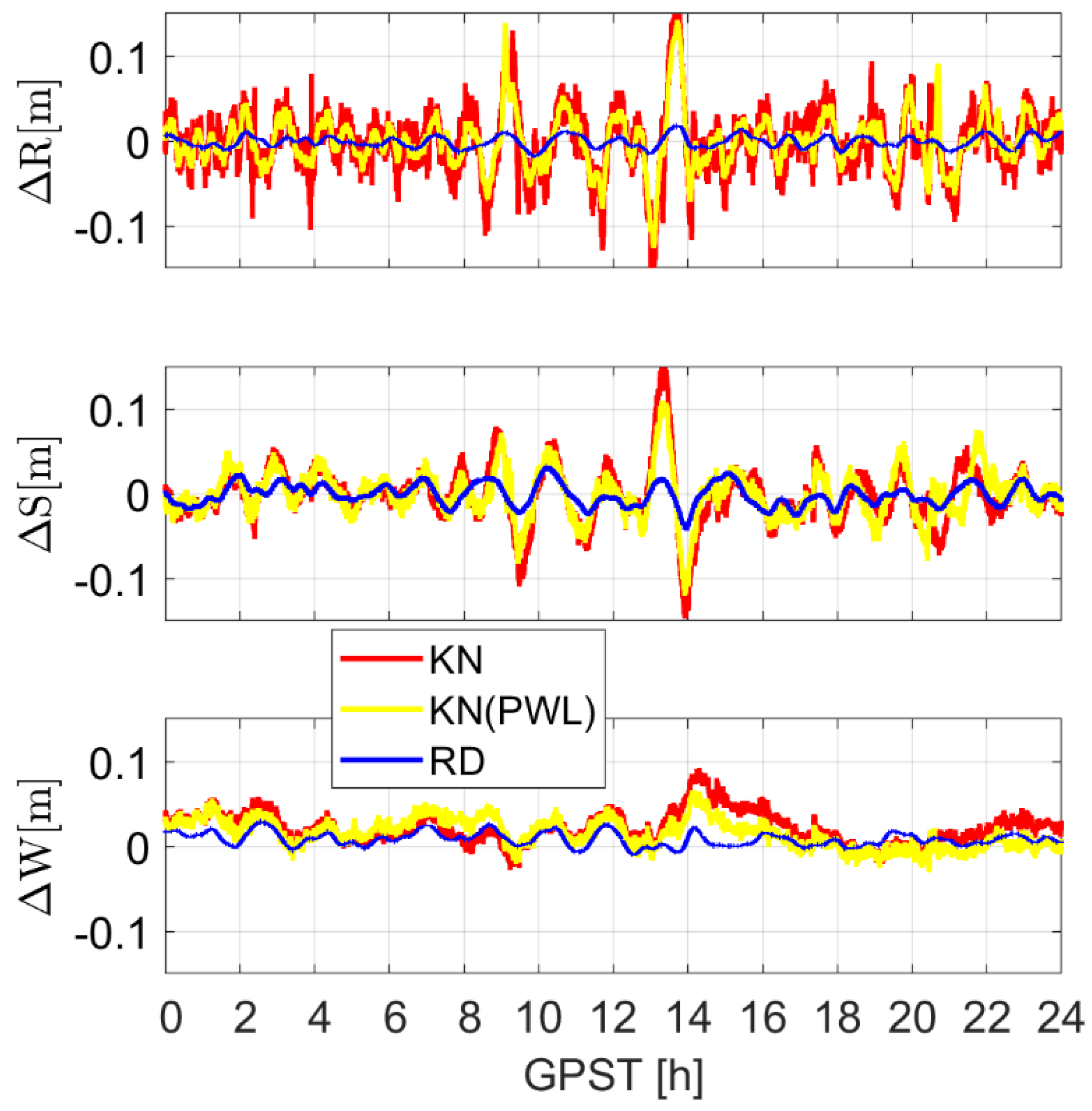
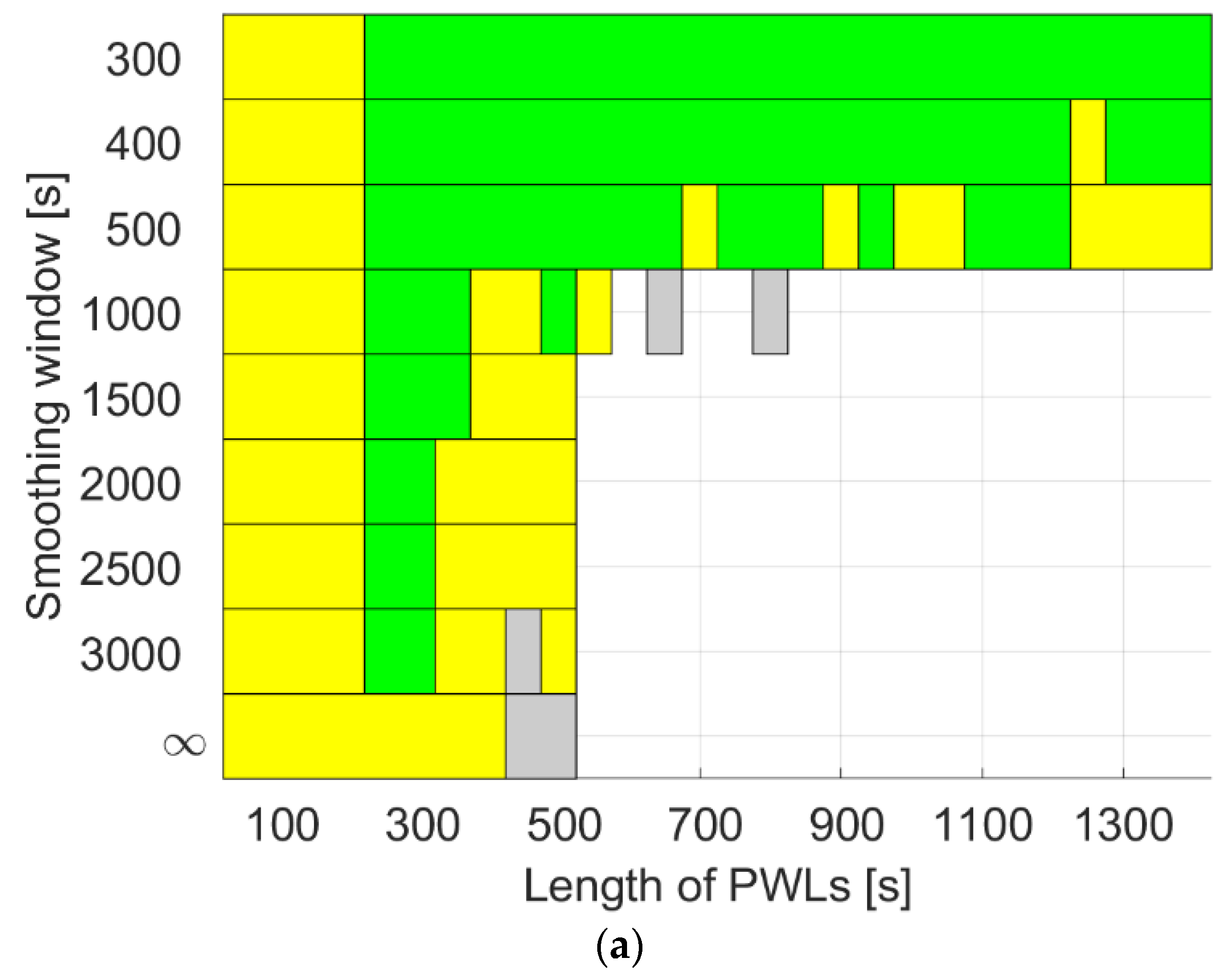
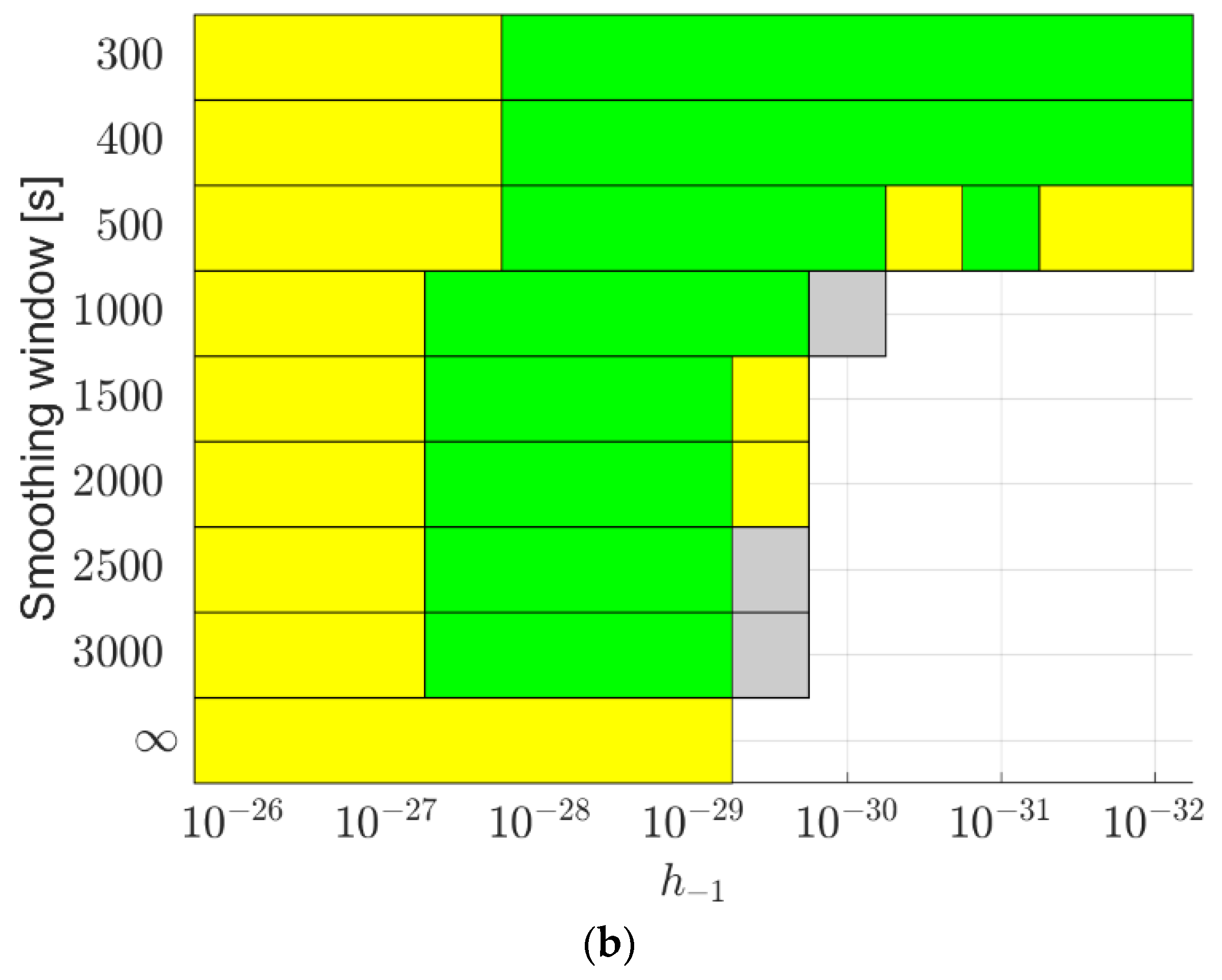
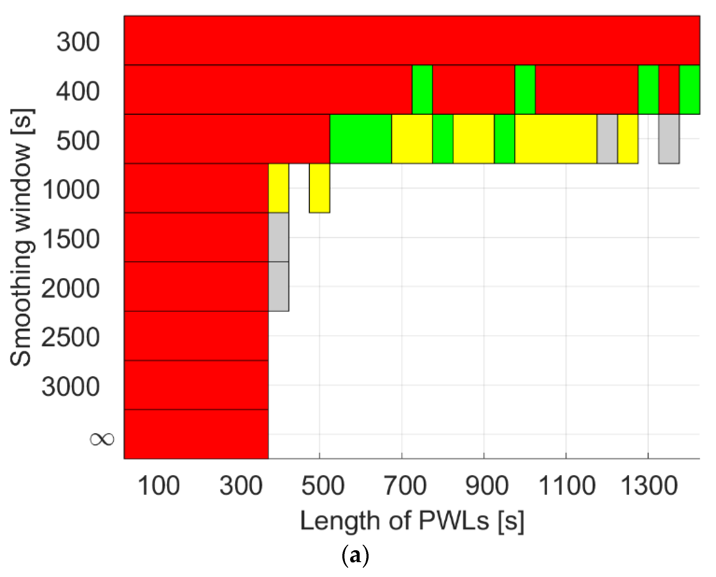
To illustrate the different effects of the PWL model and the 2.5-state model,
Figure 4 shows the estimated clock errors when applying the 2.5-state model with
s and the PWL model with
of 2000 s. Similar to
Figure 2 and
Figure 3, the satellite geometry of GRACE FO-1 on 14 August 2018 was used for the simulations, considering only the observation noise and the GPS orbital errors. As shown in
Figure 4, a small
value (
as an example) in the 2.5-state model smooths the clock estimates in the long term, while a long PWL length
extends the length of each period with infinite strong constraint, i.e., the length of the piece-wise linear polynomials. In other words, the small
value, i.e., a strong 2.5-state model, constrains and smooths the clock estimates from the short to long term. In contrast, a strong PWL model, i.e., a long PWL length
, assumes the clocks within each PWL interval to be a linear polynomial but limits these constraints within each PWL interval.


