Article

Vegetation Types Variations to the South of Ngoring Lake from 2013 to 2020, Analyzed by Hyperspectral Imaging

1
School of Land Science and Technology, China University of Geosciences (Beijing), Beijing 100083, China
2
Gansu Water Conservancy & Hydro Power Survey & Design Research Institute, No. 284, Pingliang Road, Chengguan District, Lanzhou 730030, China
3
School of Water Resources and Environment, China University of Geosciences (Beijing), Beijing 100083, China
*
Author to whom correspondence should be addressed.
Remote Sens. 2023, 15(12), 3174; https://doi.org/10.3390/rs15123174
Submission received: 18 May 2023 / Revised: 14 June 2023 / Accepted: 15 June 2023 / Published: 18 June 2023

Abstract

:
Studying the variation in vegetation types within the source region of the Yellow River (SRYR) is of great significance for understanding the response of vegetation to climate change and human activities on the Qinghai-Tibet Plateau (QTP) permafrost. In order to understand the characteristics of the variation in vegetation associations in the SRYR under the influence of climate and human activities, two hyperspectral remote sensing images from HJ-1A in 2013 and OHS-3C in 2020 were used to extract the vegetation types located in the area south of Ngoring Lake, covering 437.11 km2 in Maduo County, from the perspective of vegetation associations. Here, the hybrid spectral CNN (HybridSN) model, which is dependent on both spatial and spectral information, was used for vegetation association classifications. On this basis, the variations in vegetation associations from 2013 to 2020 were studied using the transition matrix, and the variation in noxious weeds across different altitude and slope gradients was analyzed. As an example, Thermopsis lanceolata’s spatial distribution pattern and diffusion mechanism were analyzed. The results showed that (1) in addition to noxious weeds, herbage such as Poa poophagorum, Stipa purpurea, Kobresia humilis, and Carex moorcroftii increased, indicating that the overall ecological environment tended to improve, which may be attributed mainly to the development of a warm and humid climate. (2) Most of the noxious weeds were located at low altitudes with an area increase in the 4250–4400 m altitude range and a decrease in the 4400–4500 m altitude range. More attention should be given to the fact that the noxious weeds area increased from 2.88 km2 to 9.02 km2 between 2013 and 2020, which was much faster than that of herbage and may threaten local livestock development. (3) The Thermopsis lanceolate association characterized by an aggregated distribution tended to spread along roads, herdsmen sites, and degraded swamps, which were mainly affected by human activities and swamp degradation.

1. Introduction

The source region of the Yellow River (SRYR) is an important Yellow River Basin (YRB) water conservation area [1], located in the east of the Qinghai-Tibet Plateau (QTP), covering an area of 122,000 km2. The SRYR contributes approximately 35% of the runoff to the YRB and is the main fresh water source for tens of millions of residents and agricultural irrigation in the YRB, playing an important role in regional social and economic development [2,3]. As part of the Three River Source National Park, known as ‘China’s Water Tower’, the SRYR is also of great significance to park ecological security [4].
Vegetation is a key biosphere component in supporting Earth’s biodiversity and affects many important ecosystem services, including biodiversity protection, water conservation, climate regulation, and carbon storage [5,6,7]. Vegetation, as an important part of the SRYR, can not only respond to climate change in the SRYR, but also reflect the change in the ecological environment. SRYR vegetation plays an important role in maintaining ecological environment security and sustainable development in the YRB [8]. The SRYR’s average altitude is approximately 4300 m above sea level, and the area is covered by alpine vegetation, which is among the vegetation categories most susceptible to climate change and human activities, resulting in grassland degradation or changes in vegetation communities [9,10,11,12], transforming vegetation species relationships from coexistence to competition and changing the interspecific correlation of dominant species from relevant to uncorrelated [13]. In extreme cases, degraded grasslands even evolve into ‘black soil land’. As noxious weeds have a strong ability to reproduce and compete, heavily degraded grassland is gradually dominated by noxious weeds, especially in the northern Bayan Har Mountain area and the area located near Gyaling Lake and Ngoring Lakes in the SRYR, posing a great threat to local dominant species and animal husbandry development [14]. Noxious weeds occupy a dominant position, hindering forage growth, which ultimately lead to the loss of species and ecological diversity [15]. It can also change soil nutrients, aggravate soil erosion, and eventually cause grassland desertification [16]. The SRYR is among the most sensitive and fragile ecosystems [17], and large-scale noxious weeds are bound to cause serious damage to the grasslands and the local ecosystem. Studying the variations in vegetation types is of great significance for understanding the response of vegetation to climate variation and human activities in the permafrost regions in the QTP and for strengthening the SRYR’s ecological management and protection.
Since the 1980s, many scholars have conducted in-depth research on SRYR vegetation based on multispectral satellite remote sensing data and their derived products. Previous studies have shown that vegetation activity has increased since 1980 [18]. Using the Thematic Mapper/Enhanced Thematic Mapper (TM/ETM) data from 1986 to 2000, Wang et al. believed that alpine meadow vegetation coverage had a significant downward trend with QTP permafrost active layer thickening [19]. Zhao et al. believed that the alpine meadow grassland degradation was obvious and the livestock number was significantly related to the Normalized Difference Vegetation Index (NDVI), and speculated that the main reason for grassland degradation was long-term grassland overgrazing [20]. Liu and Yang found that since the 21st century, the overall SRYR NDVI had increased, but there were obvious spatial distribution differences, mainly characterized by a gradual decrease from the southeast to northwest. For example, there was an obvious downward trend in Maduo County from 1998 to 2007 [21,22]. The SRYR NDVI change was related mainly to precipitation, temperature, and human activities. Precipitation and temperature had a positive NDVI impact, while human activities had a negative impact [23]. The SRYR vegetation was restored as a whole and the ecological protection project played an important role [23,24]. However, the above research is limited by the multispectral remote sensing spectral resolution and mainly uses the vegetation index product rather than the vegetation type succession to describe the SRYR vegetation degradation.
Hyperspectral remote sensing technology development and data accumulation provide more accurate vegetation classification and variation research possibilities. Compared to multispectral remote sensing images, hyperspectral remote sensing images have higher spectral resolution, richer spectral information, and image and spectral integration characteristics, which can identify more detailed differences among complex objects [25]. Using hyperspectral images as the main data source, An et al. extracted the composition information of edible grasses, noxious weeds, and bare soil in a typical area of the Three River Source Region based on the multiple endmember spectral mixture analysis (MESMA) algorithm and found that grassland degradation was serious in 2012 through the composition change [26]. Grassland degradation and the reproduction of noxious weeds are complementary [27]. The degradation of grassland leads to the sharp reduction in herbage and the increase in noxious weeds. The increase in noxious weeds is realized through the mutual transformation of individual assistance and community competition. The type of association with herbage as the dominant species is changed to that with noxious weeds as the dominant species. The formation of the association type with noxious weeds as the dominant species promotes the gradual consolidation and expansion of noxious weeds from scattered patches, which eventually lead to the serious degradation of grassland. It will cause serious economic losses to sustainable grassland ecosystem development when it reaches a certain scale. Few studies have focused on the noxious weed spatial distribution pattern changes and expansion mechanisms in the SRYR. It is urgent to analyze the changes in noxious weed spatial distribution patterns and the diffusion trend in the SRYR to provide a basis for future grassland protection.
The analyses of the spatial variation in vegetation association are based on the extraction of accurate vegetation types. Vegetation classifications based on hyperspectral images have been developed. Machine learning algorithms such as the support vector machine (SVM) [28] and the random forest (RF) [29] have achieved satisfactory classification accuracy, but the selection of the kernel function and optimal parameter combination was still difficult [30]. At the same time, Convolutional Neural Networks (CNNs) [31] and other deep learning (DL) algorithms or methods were applied to hyperspectral image classification or target mapping. For example, besides super-resolution mapping (SRM) based on spatial–spectral correlation (SSC) [32] and target-constrained interference-minimized band selection (TCIMBS) [33], 2D-CNN extracts spatial features of images based on 1D-CNN [34] and 3D-CNN extracts spatial and spectral features of images simultaneously on the basis of 2D-CNN, which is more suitable for hyperspectral image classification [35]. It also increases the complexity of the computational processes and the model parameters.
Our study aims to: (1) investigate the variations in vegetation types within the SRYR from the perspective of vegetation associations, especially the variations in herbage and noxious weeds that herdsmen are more concerned about; (2) investigate the spatial distribution pattern of noxious weeds, as well as their characteristics of expansion, to provide a theoretical basis for the further development of animal husbandry. In this paper, two-period spaceborne hyperspectral remote sensing images separately acquired by HJ-1A in 2013 and OHS-3C in 2020 were used to extract vegetation types in view of vegetation associations near southern Ngoring Lake. On this basis, the conversion of vegetation associations was carried out using the transition matrix, and the variation in noxious weeds was analyzed across altitude and slope gradients. In particular, the changes in the spatial distribution pattern and the expansion mechanism of a typical noxious weed, Thermopsis lanceolata, were further studied to provide decision-making support for the protection of the ecological environment and the development of animal husbandry in the SRYR.

2. Materials and Methods

2.1. Study Area

Taking into account the availability of hyperspectral remote sensing data, a small part of the SRYR covering typical alpine vegetation was selected as the study area, located near the south of Ngoring Lake, Qinghai Province, China (Figure 1). The area is between 36°15′–38°20′N and 97°50′–101°20′E and covers 437.11 km2. It belongs to the semiarid and semihumid subtropical zone and is characterized by a typical plateau climate with short, humid, and rainy summers and long, cold, and dry winters. The annual temperature in the watershed ranges from 24.3 to −48.1 degrees Celsius, and the annual precipitation is approximately 332.5 mm, occurring mostly from June to September [36]. The main soil types are aeolian sandy soil, castanozems, meadow soil, and frigid calcic soil. Vegetation types are diverse, consisting mainly of alpine grassland vegetation, alpine meadow vegetation, aquatic vegetation, alpine swamp vegetation, and cushion vegetation [23].

2.2. Data and Preprocessing

There were three hyperspectral remote sensing image scenes available that covered the study area, as shown in Table 1.
The Hyper-Spectral Imager (HSI) image with a 5 nm spectral resolution was obtained from the China Resources Satellite Application Center (www.cresda.com (accessed on 20 September 2021)) data sharing platform, while the Advanced Hyper-Spectral Imager (AHSI) image with a 5 to 10 nm spectral resolution and the Complementary Metal-Oxide-Semiconductor (CMOS) image with a 2.5 nm spectral resolution were purchased from image sales companies. As the products were subjected to radiative and system geometry corrections, the image was then preprocessed with band removal, bad line repair, stripe removal, atmospheric correction, and geometric correction [37,38]. All the processing was performed using ENVI 5.3 software.
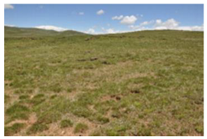
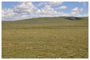
Field data collection was conducted to explore and verify the vegetation type in July and August when the vegetation grew best from 2019 to 2021. In order to determine the vegetation types accurately in the study area, we used random sampling. First, we set-up a 10 m × 10 m plot at each sample site. For each sample plot, a total of 5 1 m × 1 m quadrats were set at four corners and the central position, and the GPS coordinates of the central quadrats were measured by Trimble Geo XH 6000 hand-held GPS(made by Beijing Mingtu Technology Co., Ltd., Beijing, China) units with an accuracy of 0.1 m. For each quadrat, it was photographed and the vegetation cover of each species was estimated and recorded. The five quadrats were averaged to determine the dominant species within the plot. The coverage of the sample sites in the study area is affected by accessibility (wetlands and lakes could not be entered), by the inadaptation of researchers at high altitudes and low atmospheric pressure, as well as by dangerous animals such as wolves and yaks [39]. We were able to investigate most of the north of the main road and a little of south and collected a total of 45 points (Figure 1). A typical sample of each vegetation type is selected for display (Table 2).
In addition, a 1:1,000,000-scale vegetation-type database covering the study area released by the Chinese QTP Data Center was used to provide a spatial vegetation distribution overview.
To explore causes of vegetation types variations, 1 km MODIS land surface temperature data from 2013 to 2020 after processing [40]; precipitation data from four meteorological observation stations in Dulan, Maduo, Dari, and Qumalai of Qinghai Province from 2013 to 2020 (http://www.ncdc.noaa.gov/ (accessed on 10 October 2022)); land use type classification data from 2013 and 2020 [41]; and Advanced Spaceborne Thermal Emission and Reflection Radiometer (ASTER) Global Digital Elevation Model (GDEM) data with a 30 m spatial resolution per pixel (http://www.gscloud.cn/ (accessed on 30 October 2022)) were collected. The precipitation distribution map covering the study area was obtained from the precipitation data of four stations by the inverse distance weighting method. The DEM was resampled to 100 m and 10 m with the same resolution as the HJ-1A and OHS-3C images, and the elevation and slope layers of the study area were calculated by the DEM.

2.3. Methods

2.3.1. Hybrid Spectral Convolutional Neural Network (HybridSN)

DL has become very widespread for classification or image feature extraction application and has shown a high-performance capability. CNNs are one of the most popular utilized DL networks [42]. CNN takes the original data as input, reduces the data reconstruction based on ensuring data integrity, and has the advantage of automatic extraction of vegetation features [43]. CNN contains mainly 2D-CNN and 3D-CNN. The 2D-CNN can use a 2D convolution kernel to extract the spatial features of multispectral remote sensing images to identify complex ground objects. However, the feature extraction mechanism is insufficient to extract rich spectral information, and there are problems such as multiple network parameters and high computational cost. As a transformation form of ordinary 2D-CNN, depthwise separable convolution (DSC) improves the problems of a large number of parameters and a high computational cost and, in practice, improves the practicability of network classification models [44]. The 3D-CNN uses 3D convolution kernels to extract hyperspectral images’ spatial and spectral features fully and improves the network model vegetation types’ classification accuracy [30]. However, it also improves the complexity and computational complexity of the network model and puts forward higher requirements for computer performance in practical applications. The HybridSN model is composed of 2D-CNN and 3D-CNN, which maximizes the extraction accuracy and reduces the model complexity and computational complexity on the basis of the simultaneous extraction of spatial–spectral joint information of images [45].
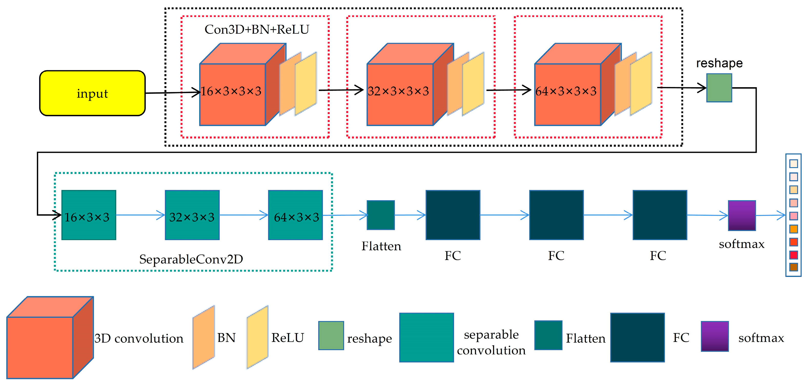
In our study, we applied a HybridSN model that combined 3D-CNN and DSC to extract vegetation types (Figure 2). The HybridSN model contained a 3D feature extraction block (black box), a 2D feature extraction block (green box), a flatten layer, three fully connected (FC) layers, and a softmax classifier. The 3D feature extraction block was composed of three small units (red box), and each small unit was made up of 3D convolution (Conv3D), a rectified linear unit (ReLU) as the activation function, and a batch normalization (BN) layer, which had the characteristics of speeding up the convergence rate, preventing overfitting, and preventing the vanishing gradient. The 3D feature extraction block was used to learn the spatial–spectral features of the image. The 2D feature extraction block (green box) consisted of three separable convolution (SeparableConv2D) layers. Two-dimensional feature blocks were used to extract more deep spatial features. In the HybridSN framework, the dimensions of the three-layer 3D convolution kernel were 16 × 3 × 3 × 3, 32 × 3 × 3 × 3, and 64 × 3 × 3 × 3, in order, where 64 × 3 × 3 × 3 means 64 3D convolution kernels of dimension 3 × 3 × 3 (one spectral dimension and two spatial dimensions). Additionally, this was then followed by three separable convolution kernels, with dimensions of 16 × 3 × 3, 32 × 3 × 3, and 64 × 3 × 3, where 64 × 3 × 3 means 64 2D convolution kernels of dimension 3 × 3 (two spatial dimension) [45]. Finally, the output number of softmax was 9, which is the same number of experimental data classes.
At the same time, for this paper, Principal Component Analysis White (PCAW) was chosen to reduce the hyperspectral image dimension before putting it into the network to prevent the ‘curse of dimensionality’ phenomenon to improve the learning speed of the network model [46]. In our paper, the HJ-1A, GF-5, and OHS-3C band dimensionalities were reduced to 60, 55, and 16 by PCAW, respectively.

2.3.2. Transition Matrix

The transition matrix can represent the mutual conversion relationship effectively between various types of vegetation in two periods and can better analyze its temporal and spatial evolution process [47]. The mathematical representation is shown in Equation (1):
K = ( k 11 k 1 j k i 1 k i j )
where K is the transition matrix from state k i to state k j .

2.3.3. Linear Regression Trend Model

The linear regression trend method is used for predicting the changing trend of variables by performing linear regression analysis on time-varying variables [48]. Its mathematical representation is shown in Equation (2):
S l o p e = n i = 1 n ( i × X i ) i = 1 n i × i = 1 n X i n i = 1 n i 2 ( i = 1 n i ) 2
where S l o p e is the slope of the regression equation, X i is the mean value of the variable in year i, and j is the length of time. The value of S l o p e is normally between [−1, 1], although when S l o p e is positive, the indicator shows an increasing trend in n years, and vice versa. When S l o p e = 0 , it does not show a trend change [49].

2.3.4. Ripley’s K Function

Ripley’s K function reflects the point events’ spatial distribution dependence [50]. Its mathematical model is shown in Equation (3):
K ( d ) = A i = 1 n j = 1 n d i j ( d ) n 2
where A represents the area of the study area, n is the total number of individuals in the study area, i and j are two individual events, d i j is the distance between two points i and j, and d is the distance scale. Generally, L ( d ) is used instead of K ( d ) , and the mathematical model is shown in Equation (4):
L ( d ) = K ( d ) π d 2
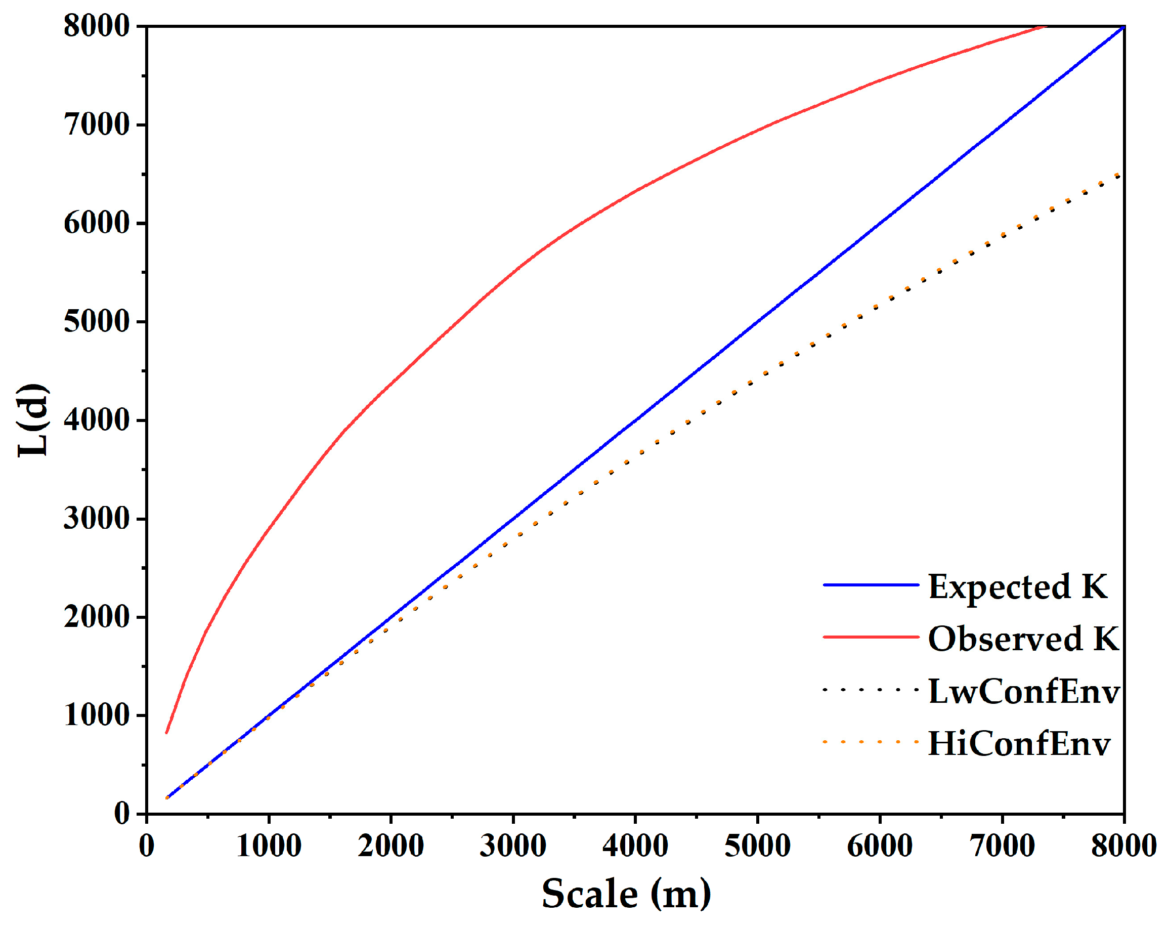
where L ( d ) is a linear transformation of K ( d ) . In the random distribution, the expected value of L ( d ) is 0. Ripley’s K function analysis and significance test are performed in ArcGIS10.2 and five parameters are generated: O b s e r v e d   K ( L ( d ) ), E x p e c t e d   K (distance d ), L w C o n f E n v (discrete confidence intervals for E x p e c t e d   K ), H i C o n f E n v (clustered confidence intervals for E x p e c t e d   K ), and D i f f K (the difference between O b s e r v e d   K and E x p e c t e d   K ).
When O b s e r v e d   K > H i C o n f E n v and O b s e r v e d   K > E x p e c t e d   K , the event shows a significant aggregated distribution. When O b s e r v e d   K < L w C o n f E n v and O b s e r v e d   K < E x p e c t e d   K , the event shows a significant uniform distribution. When O b s e r v e d   K is located between L w C o n f E n v and H i C o n f E n v , the event shows a significant discrete distribution. When D i f f K is largest, it means that the aggregated distribution is strongest, and when D i f f K is smallest, it means that the discrete distribution is strongest.

2.3.5. Nearest Neighbor Hierarchical Spatial Cluster (NNH)

The NNH identifies closed event groups in space. According to the nearest neighbor index, the multilevel spatial aggregation areas are obtained [19]. By defining the limit distance or threshold of the ‘cluster unit’, several first-level cluster units are formed. Then, the second-level cluster units are obtained by gathering the first-level clustering units. The second-level cluster units are extrapolated to higher-aggregation areas until all points are grouped into a single cluster or do not meet the cluster conditions. CrimeStat 3.3 software was used to conduct multiple experiments, and the best results were obtained. The minimum number of points was set to 5 and the standard deviation of the aggregation area ellipse was set to 1X; that is, approximately 50% of the points were included in the aggregated ellipse. The threshold is calculated by the random nearest neighbor distance method, and the mathematical model is shown in Equation (5).
R = 0.5 A N ± 1.645 0.26136 A N
where A represents the area of the region; N represents the number of events; 1.645 represents the abscissa corresponding to the 95% normal distribution range on both sides of the curve center.

3. Results

3.1. Classification of Vegetation Associations

3.1.1. Definition of Vegetation Association and Sample Selection

Various vegetation types in the study area do not exist independently but cross each other in different proportions. There are no obvious spatial boundaries in the species distribution. Furthermore, due to the remote sensing spatial resolution image limitation, the corresponding ground range represented by each pixel is a rectangular area with spatial resolution size as the side length, and the species are not a single category within the pixel. For the above reasons, this paper adopted the associations in the community classification system and determined the association types based on the type of dominant species in each association to examine the study area’s vegetation variation. After field investigation, Carex moorcroftii, Kobresia tibetica Maxim association; Kobresia humilis, Leontopodium pusillum association; Kobresia humilis, Stipa purpurea association; Poa poophagorum, Stipa purpurea association; the Stipa purpurea association; Stipa purpurea, Leontopodium pusillum association; noxious weeds; water; and bare ground were selected. Specific vegetation association information is shown in Table 3.
The selection of training and test samples was based on the principles of typicality, representativeness, and appropriateness with the help of field survey data and vegetation type databases at a scale of 1:1,000,000. Based on 1:1,000,000-scale vegetation-type databases, field survey data, and GF-2 data with 1 m resolution, labels were selected on hyperspectral images such as OHS-3C, GF-5, and HJ-1A. The proportion of training samples and test samples was sat at 70% and 30%, respectively. The numbers of training and test samples are shown in Table 4.

3.1.2. Vegetation Association Classification Results

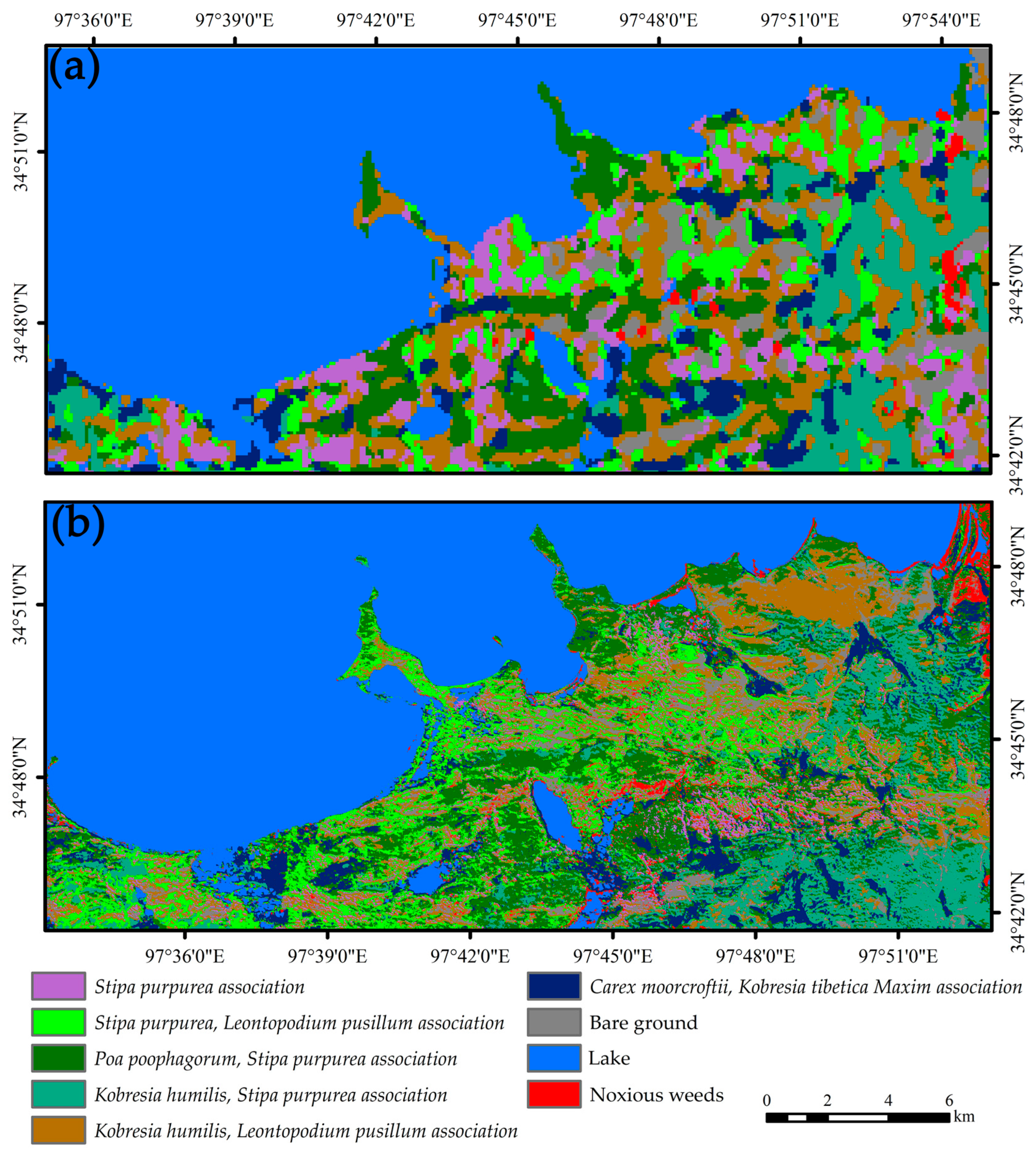
In the HybridSN model, the window size was set to 9, the batch size was set to 128, the iteration number was set to 150, and the weights were used and initialized to obtain the best classification results after experimentation. The Kappa coefficients of HJ-1A, GF-5, and OHS-3C were 0.9911, 0.9904, and 0.9931, respectively, and the overall accuracies were 99.23%, 99.29%, and 99.70%, respectively. The accuracy obtained by HybridSN was much higher than that of support vector machine (SVM). The user’s accuracy (UA) and producer’s accuracy (PA) of each category are shown in Table 5. The classification and the area statistics results are shown in Figure 3 and Table 6, respectively.

3.2. Classification Accuracy Verification

In addition to Kappa coefficients and overall accuracies, we verified the accuracy of the extracted vegetation associations in two other ways: data collected from field surveys and vegetation association comparisons in neighboring years.
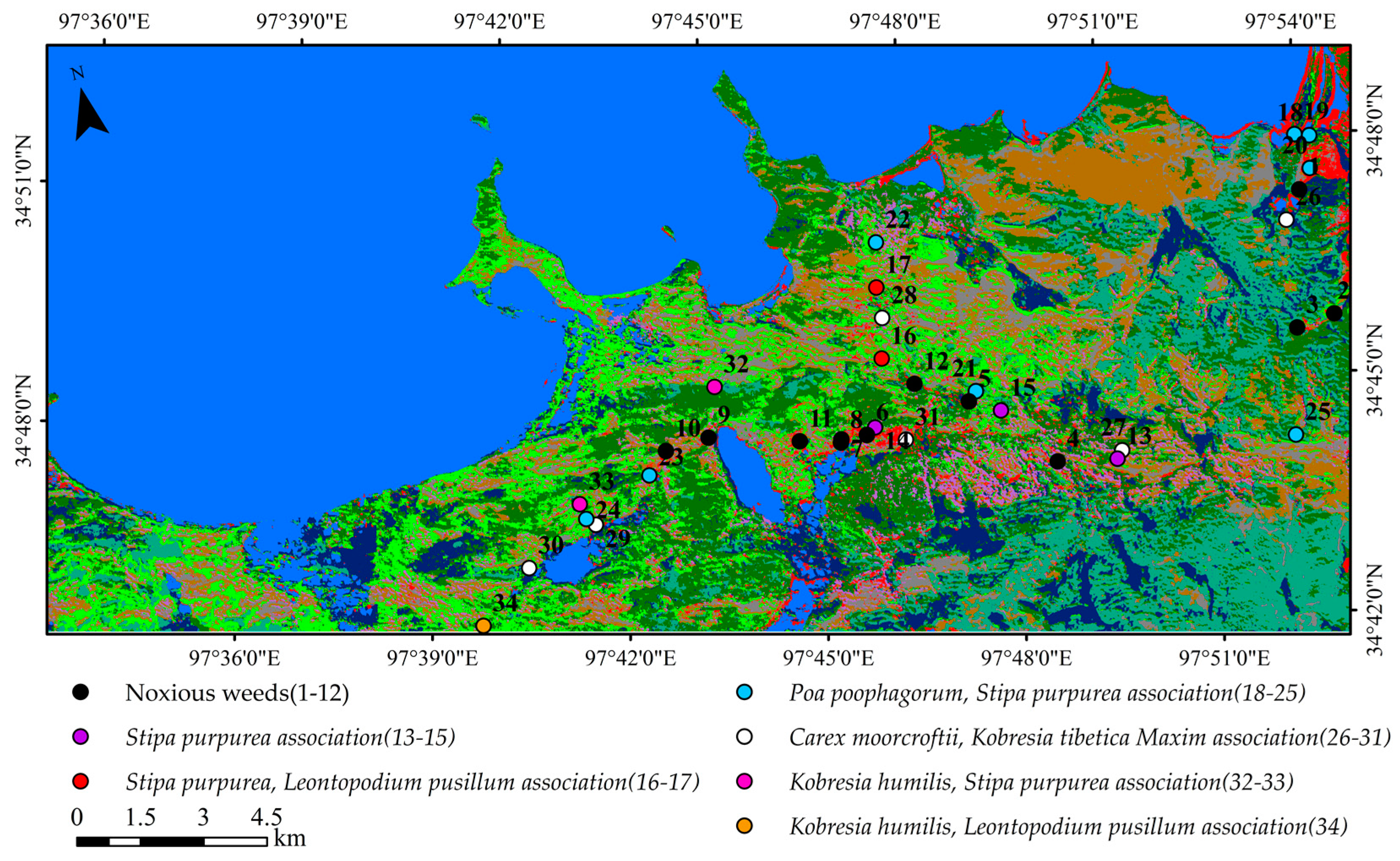
Through field investigation in the study area, a total of 34 in situ verification points were selected to verify the 2020 OHS-3C vegetation association extraction results. Point-by-point inspection results showed that the vegetation types were fully compatible with the field vegetation types. The actual verification point distribution is shown in Figure 4.
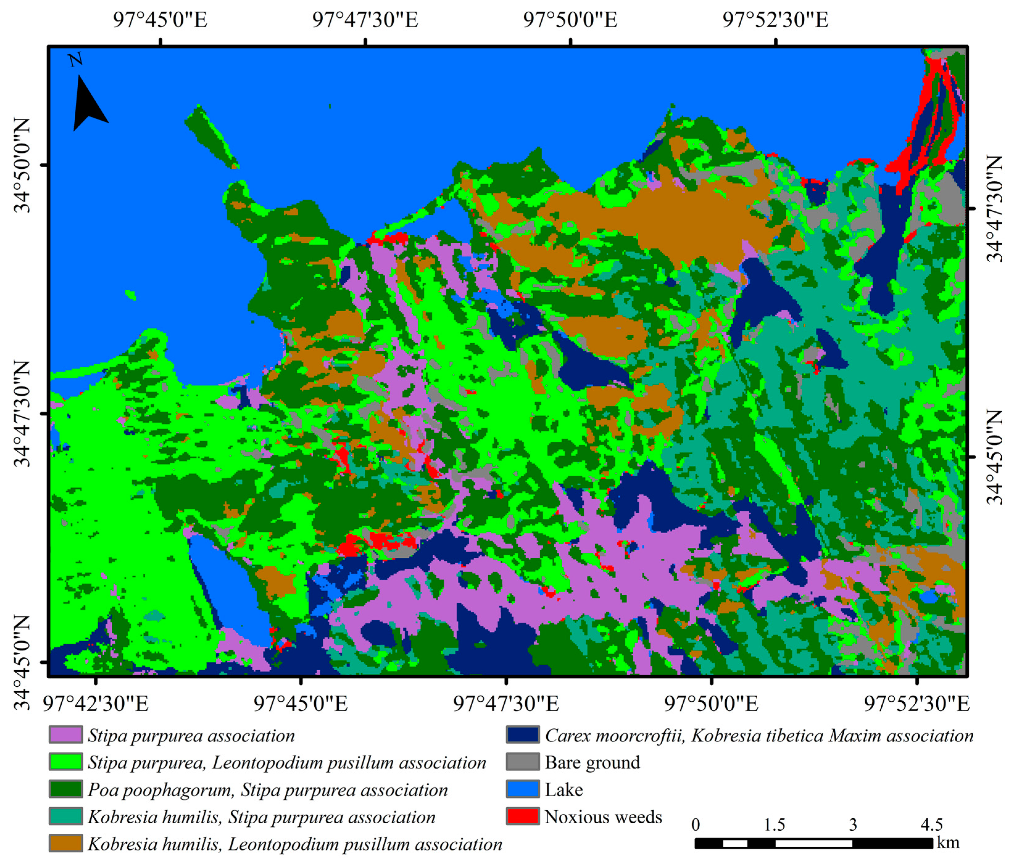
The main vegetation type in the study area was perennial vegetation. Assuming that there was little spatial vegetation distribution variation between adjacent years, the 2019 GF-5 vegetation extraction results were used as a reference to verify the 2020 OHS-3C extraction results in the same area (Figure 5). According to the 2019 and 2020 vegetation type extraction results (Table 7), the difference between the vegetation association proportions was less than 5% in the two periods, which could indicate that the vegetation association spatial distribution had no variation in the two years adjacent to 2019 and 2020.

3.3. Vegetation Association Variation Analysis

Comparing the 2020 extraction result with that in 2013, the lake; bare ground; the Stipa purpurea association; and Kobresia humilis, Leontopodium pusillum association areas decreased (Table 5). The area of high-quality grasses for livestock, such as Carex moorcroftii, Kobresia tibetica Maxim association; Poa poophagorum, Stipa purpurea association; Kobresia humilis, Stipa purpurea association; the Stipa purpurea association; and Stipa purpurea, Leontopodium pusillum association increased. At the same time, the noxious weeds area also significantly increased, among which the growth rate of the decrease in the Stipa purpurea association area was largest, while the growth rate of the increase in the noxious weeds area was largest, followed by Poa poophagorum, Stipa purpurea association.
The transition matrix follows for the decreased land cover conversion, the decrease in lake area was transformed into Poa poophagorum, Stipa purpurea association; Stipa purpurea, Leontopodium pusillum association; Carex moorcroftii, Kobresia tibetica Maxim association and some noxious weeds. The decrease in bare ground was transformed into Kobresia humilis, Leontopodium pusillum association and Stipa purpurea, Leontopodium pusillum association. The decrease in the Stipa purpurea association was transformed into Kobresia humilis, Leontopodium pusillum association; Stipa purpurea, Leontopodium pusillum association; and Poa poophagorum, Stipa purpurea association. The decrease in the area of Kobresia humilis, Leontopodium pusillum association was transformed into Poa poophagorum, Stipa purpurea association; Stipa purpurea, Leontopodium pusillum association; and some Kobresia humilis, Stipa purpurea association. The detailed conversions among various vegetation associations are shown in Table 8 and Figure 6.

3.4. Temperature and Precipitation Trend Analysis

The vegetation variation is influenced by climatic and nonclimatic factors. Based on the analysis of the surface temperature and annual precipitation change trend in the study area from 2013 to 2020 (Figure 7), it was found that surface temperature and annual precipitation increased and continued to increase in the study area, and the climate tended to increase temperature and humidity.

3.5. Noxious Weed Variation across Altitude and Slope Gradients

As there were no noxious weeds beyond the 25-degree slope, the grassland slopes were divided into two levels, 0–7° and 7–25°, which were denoted as the bottomland and gentle slope, respectively, considering the SRYR terrain conditions of and the engineering management needs (Table 9) [51], while the altitude gradient was divided into seven grades at an interval of 50 m (Table 10), which were 4200–4250 m, 4250–4300 m, 4300–4350 m, 4350–4400 m, 4400–4450 m, 4450–4500 m, and 4500–4550 m, as indicated by Ⅰ-Ⅶ from low to high.
The noxious weed distribution was counted at both different altitudes and slopes levels in 2020, as shown in Figure 8. More than 80% of the noxious weeds were distributed in the altitude range of 4250–4350 m, and the proportion in the bottomland was much higher than that in the gentle slope in this range. The noxious weeds proportion distribution was less in the area with altitudes over 4350 m and showed a decreasing trend with an increasing altitude, but the gentle slope distribution proportion was higher than in the bottomland. The noxious weeds spatial distribution pattern was significantly affected by altitude and slope.
The variations in area of noxious weeds with altitude gradient in 2013 and 2020 are shown in Figure 8. There was little variation in the noxious weeds in the altitude ranges of 4200–4250 m and 4500–4550 m from 2013 to 2020. Noxious weeds increased to a large area in the range of 4250–4400 m between 2013 and 2020, with the largest increase between 4250 and 4300 m. The noxious weeds area decreased gradually in the altitude range of 4400–4500 m, with the largest decrease between 4450 and 4500 m.

3.6. Thermopsis Lanceolata Association Spatial Distribution Pattern

As a typical noxious weed, Thermopsis lanceolata is distributed widely in the study area and is characterized by aggregation. Once occurring, it presents a grassland landscape with a patchy association dominated by Thermopsis lanceolata. This poses a greater threat to animal husbandry development, so the extraction result of Thermopsis lanceolata was used to analyze the spatial distribution and diffusion characteristics as a typical example (Figure 9). Its area was 3.18 km2, accounting for 33% of the total noxious weeds area.
Ripley’s K function result of the Thermopsis lanceolata association is shown in Figure 10. The points of the Thermopsis lanceolate association showed an aggregated distribution pattern on the 0–8 km scale. The aggregated degree was high, among which the best aggregation state was on the 3 km scale.

3.7. Thermopsis Lanceolata Association Diffusion Mechanism Analysis

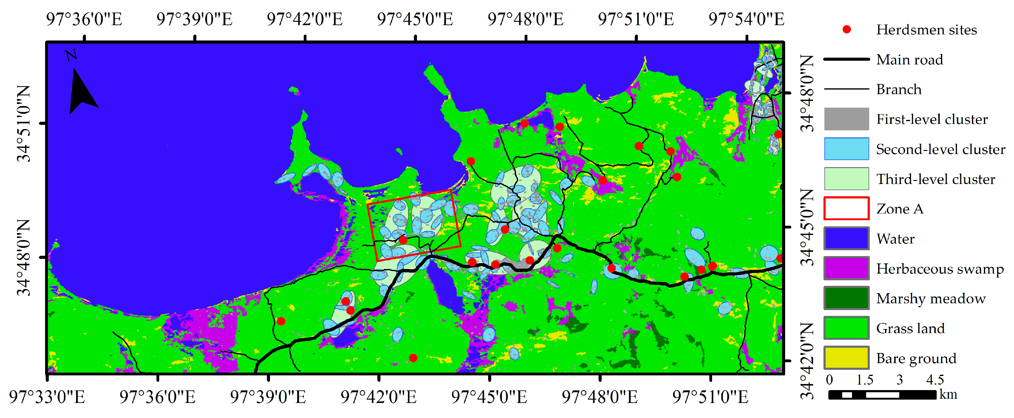
The NNH result of the Thermopsis lanceolate association is shown in Figure 11. There were three spatial cluster levels. The first-level cluster represented the spatial aggregation of Thermopsis lanceolata pixels. It presented a large number of patches, most of which were distributed in the northeast and central regions, and the rest were located in the eastern, southwestern, and southern regions of the study area. It appears that the overall spatial distribution was random. The second-level cluster was the local aggregation region of Thermopsis lanceolata patches, which were concentrated on both sides of the road, around the herdsmen sites, and in the waterside areas such as the herbaceous swamp. The third-level cluster represented the second-level cluster spatial concentration area, that is, the large-scale Thermopsis lanceolata patch area. The third-level cluster showed an obvious zonal distribution with roads and herdsmen sites, and was diffused around swamps—denoted as zone A. The third-level cluster had a clear trend of extending along the road to the east in the northeast and along the road to the southwest in the middle.
It was found that the Thermopsis lanceolata association gathered on both sides of the road, around the herdsmen sites, and around the herbaceous swamp primarily according to the diffusion mechanism. The expansion directions were spread along the road and around the herdsmen sites near the roads, as well as to the surrounding swamps. There are three explanations for this phenomenon:
The first is that human transport caused the Thermopsis lanceolata association diffusion [52]. Vehicles could be used as a temporary habitat for biological seeds, bringing seeds from one place to another. It provided a diffusion opportunity for adaptive and reproductive Thermopsis lanceolata.
The second is that the Thermopsis lanceolata diffusion was mediated by animals [53]. During grazing, livestock ruminated or defecated the seeds so that seeds spread and grew around the herdsmen sites and along roads. With its strong production capacity and the ability of roots to erode water and heat resources [54], Thermopsis lanceolata occupied most of the grassland resources gradually and replaced forage as the dominant species.
The last is the shrinkage of marshes. Thermopsis lanceolate had an increasing trend of aggregation in a degraded swamp. According to the land cover extraction in zone A in 2013 and 2020 (Table 11), we found that the area of herbaceous marshes shrank significantly, with an area reduction of approximately 31% from 2013 to 2020. Permafrost degradation contributes to swamp degradation [55]. With the aggravation of wetland degradation, the soil pH increased and showed a salinization trend. The abilities of forage plants to absorb and utilize soil nutrients were weakened, while Thermopsis lanceolata had a strong ability to adapt to adverse environments, grew well in alkalized and salinized soils, and maintained the content of elements in the roots by increasing organic matter [56]. Moreover, the allelopathic effect of Thermopsis lanceolata inhibited seed germination and growth of the forage [57]. For the above reasons, it expanded widely in zone A shown in Figure 11.

4. Discussion

4.1. Influencing Factors of Vegetation Association Variation

The classification results from 2013 and 2020 showed that the area of vegetation association increased or decreased, and most of the area increased in the study area. Temperature and precipitation are one of the factors affecting vegetation variation. Figure 7 showed that the annual precipitation and surface temperature show an increasing trend in the study area, and the climate gradually becomes warm and humid. This climatic conditions were conducive to vegetation restoration [58,59], so the area of vegetation associations increased. However, there were also some associations that had decreased. Because the study area belonged to alpine permafrost areas, the interaction between climate and frozen soil might be the reason for the decrease. Human activities also played a role. For example, although precipitation had increased, the area of the lake still decreased. Because the hydropower station had been dismantled at the mouth of Ngoring Lake, its water storage function had failed, resulting in a decrease in the lake area. In the next section, we discuss the impact of human activities on the variation in noxious weeds along with the terrain, reflecting the corresponding role of human activities.

4.2. Spatial Distribution and Diffusion of Noxious Weeds

Noxious weeds were among the most obvious variations in vegetation association. Although the growth area is small, the growth rate is far higher than that of high-quality grass. It was found that the distribution of noxious weeds was limited by terrain conditions. It is mainly distributed in low altitude areas, and the area gradually decreases with increasing altitude, which is the same as the conclusion of Xing et al [27]. From 2013 to 2020, the largest increase in noxious weeds was found at lower altitudes. The study also found that the distribution of noxious weeds was also associated with human activity region, mainly on both sides of the road, around the herdsmen sites, and around the herbaceous swamp. The above areas were located mostly in the low-altitude area, which explained the phenomenon of the large area increase in noxious weeds at low altitudes. There were fewer human activity interventions in the high-altitude area, so the area of noxious weeds decreased and the overall ecological environment improved, which proved from the side that human activities mainly caused the variation in vegetation associations dominated by grassland degradation.

4.3. Future Research Direction

At present, most studies focus on vegetation index and lack of vegetation association in the SRYR. In this paper, with vegetation association as the classification unit, the deep learning method can achieve good classification results on HJ-1A, GF-5 and OHS-3C. However, there are few hyperspectral remote sensing images available in the SRYR, which makes it difficult to study the vegetation types variations at a large scale using time series data. Moreover, there are few hyperspectral remote sensing images available in the SRYR, which makes it difficult to study the vegetation types variations at a large scale using time series data. Moreover, due to the different HJ-1A and OHS-3C images resolutions, the extraction results may suffer from a scale discrepancy and spectral mixtures [60,61]. Integrating UAV and ground spectrometer measurements with the satellite images would be a further research topic.

5. Conclusions

In this paper, two-period spaceborne hyperspectral remote sensing images acquired by HJ-1A HSI in 2013 and OHS-3C in 2020 were used to extract vegetation types near southern Ngoring Lake. On this basis, the vegetation type variations and its causes were explored. We analyzed the noxious weeds distribution characteristics in view of altitude and slope. As a typical noxious weed, the Thermopsis lanceolata association was selected to further study the spatial distribution pattern and diffusion mechanism of noxious weeds by Ripley’s K function and the NNH method. The following conclusions were obtained:
  • The vegetation cover area increased, where the noxious weeds area increased more rapidly. The surface temperature and annual precipitation increases were conducive to vegetation restoration, while human activities had the opposite effect on vegetation.
  • The noxious weeds area decreased gradually with increasing altitude. Most of noxious weeds were located in the bottomland or on the gentle slope of 4250–4350 m. The noxious weeds area increased in the range of 4250–4400 m from 2013 to 2020, and the increase was highest at 4250–4300 m. The noxious weeds area decreased mainly at 4400–4500 m, and the decrease was largest in the range of 4450–4500 m.
  • The Thermopsis lanceolata association distribution was characterized by aggregation, and its diffusion direction was mainly along the road and the herdsmen sites located near the road and around the swamp. The diffusion was attributed to human activities such as human transportation, overgrazing, or the degradation of swamp wetlands.

Author Contributions

Conceptualization, X.L. and G.W.; methodology, X.L.; software, X.L. and Y.S.; validation, X.L., Y.S., and J.J.; formal analysis, X.L.; investigation, X.L., Y.S., G.W., and S.L.; resources, G.W. and S.L.; data curation, J.J.; writing—original draft preparation, X.L.; writing—review and editing, G.W.; visualization, Y.S.; supervision, J.J.; project administration, G.W.; funding acquisition, G.W. All authors have read and agreed to the published version of the manuscript.

Funding

This work was supported by the Strategic Priority Research Program of the Chinese Academy of Sciences (XDA20100103), and the Applied Fundamental Research Foundation of Qinghai Province in China (2017-ZJ-743).

Acknowledgments

We express our heartfelt gratitude for Zhihai Yang and Fang Li for our work of field sample collection. We would like to thank anonymous reviewers for their constructive input in the manuscript.

Conflicts of Interest

The authors declare no conflict of interest.

References

  1. Liu, Q.G.; Huang, Y.F. Spatial and temporal changes and driving factors of desertification in the Source Region of the Yellow River, China. Nat. Environ. Pollut. Technol. 2020, 19, 1435–1442. [Google Scholar] [CrossRef]
  2. Lan, Y.C.; Zhao, G.H.; Zhang, Y.N.; Wen, J.; Liu, J.Q.; Hu, X.L. Response of runoff in the source region of the Yellow River to climate warming. Quat. Int. 2010, 226, 60–65. [Google Scholar] [CrossRef]
  3. Hu, Y.R.; Maskey, S.; Uhlenbrook, S.; Zhao, H.L. Streamflow trends and climate linkages in the source region of the Yellow River, China. Hydrol. Process. 2011, 25, 3399–3411. [Google Scholar] [CrossRef]
  4. Liu, L.L.; Sayer, E.J.; Deng, M.F.; Li, P.; Liu, W.X.; Wang, X.; Yang, S.; Huang, J.S.; Luo, J.; Su, Y.J.; et al. The grassland carbon cycle: Mechanisms, responses to global changes, and potential contribution to carbon neutrality. Fundam. Res. 2022, 3, 209–218. [Google Scholar] [CrossRef]
  5. Ibarra-Manriquez, G.; González-Espinosa, M.; Martínez-Ramos, M.; Meave, J.A. From vegetation ecology to vegetation science: Current trends and perspectives. Bot. Sci. 2022, 100, S137–S174. [Google Scholar] [CrossRef]
  6. Wang, D.N.; Zhao, Y.T.; Yang, W.X.; Ma, K.X.; Hao, T.X.; Zhao, J.W.; Tang, R.; Pu, Y.F.; Zhang, X.J.; Mujtaba, K.G.; et al. Ecological–economic assessment and managerial significance of water conservation in the Headwaters of the Yellow River. Water 2022, 14, 2553. [Google Scholar] [CrossRef]
  7. Wei, Y.Q.; Wang, W.W.; Tang, X.J.; Li, H.; Hu, H.W.; Wang, X.F. Classification of alpine grasslands in cold and high altitudes based on multispectral Landsat-8 images: A case study in Sanjiangyuan National Park, China. Remote Sens. 2022, 14, 3714. [Google Scholar] [CrossRef]
  8. Liu, X.F.; Zhang, J.S.; Zhu, X.F.; Pan, Y.Z.; Liu, Y.X.; Zhang, D.H.; Lin, Z.H. Spatiotemporal changes in vegetation coverage and its driving factors in the Three-River Headwaters Region during 2000–2011. J. Geogr. Sci. 2014, 24, 288–302. [Google Scholar] [CrossRef]
  9. Verrall, B.; Pickering, C.M. Alpine vegetation in the context of climate change: A global review of past research and future directions. Sci. Total Environ. 2020, 748, 141344. [Google Scholar] [CrossRef]
  10. Salhab, J.; Wang, J.L.; Anjum, S.A.; Chen, Y.X. Assessment of the grassland degradation in the southeastern part of the source region of the Yellow River from 1994 to 2001. J. Food Agric. Environ. 2010, 8, 1367–1372. [Google Scholar]
  11. Yi, X.S.; Li, G.S.; Yin, Y.Y. The impacts of grassland vegetation degradation on soil hydrological and ecological effects in the source region of the Yellow River--A case study in Junmuchang region of Maqin country. Procedia Environ. Sci. 2012, 13, 967–981. [Google Scholar] [CrossRef] [Green Version]
  12. Qin, Q.T.; Chen, J.J. Research on the variation characteristics of vegetation change and its terrain influence factors in alpine grassland in the Source Region of the Yellow River. Int. Arch. Photogramm. Remote Sens. Spat. Inf. Sci. 2020, XLII-3/W10, 479–485. [Google Scholar] [CrossRef] [Green Version]
  13. Hu, Y.; Wang, H.; Jia, H.; Pen, M.; Liu, N.; Wei, J.; Zhou, B. Ecological niche and interspecific association of plant communities in alpine desertification grasslands: A case study of Qinghai Lake Basin. Plants 2022, 11, 2724. [Google Scholar] [CrossRef]
  14. Callaway, R.M.; DeLuca, T.H.; Belliveau, W.M. Biological-control herbivores may increase competitive ability of the noxious weed Centaurea Maculosa. Ecology 1999, 80, 1196–1201. [Google Scholar] [CrossRef]
  15. Rocchini, D.; Andreo, V.; Förster, M.; Garzon-Lopez, C.X.; Gutierrez, A.P.; Gillespie, T.W.; Hauffe, H.C.; He, K.S.; Kleinschmit, B.; Mairota, P. Potential of remote sensing to predict species invasions: A modelling perspective. Prog. Phys. Geogr. 2015, 39, 283–309. [Google Scholar] [CrossRef] [Green Version]
  16. Li, Y.Y.; Dong, S.K.; Liu, S.L.; Wang, X.X.; Wen, L.; Wu, Y. The interaction between poisonous plants and soil quality in response to grassland degradation in the alpine region of the Qinghai-Tibetan Plateau. Plant Ecol. 2014, 215, 809–819. [Google Scholar] [CrossRef]
  17. Liu, J.; Chen, J.J.; Qin, Q.T.; You, H.T.; Han, X.W.; Zhou, G.Q. Patch pattern and ecological risk assessment of alpine grassland in the Source Region of the Yellow River. Remote Sens. 2020, 12, 3460. [Google Scholar] [CrossRef]
  18. Piao, S.L.; Mohammat, A.; Fang, J.Y.; Cai, Q.; Feng, J.M. NDVI-based increase in growth of temperate grasslands and its responses to climate changes in China. Glob. Environ. Chang.-Hum. Policy Dimens. 2006, 16, 340–348. [Google Scholar] [CrossRef]
  19. Wang, G.X.; Li, Y.S.; Wu, Q.B.; Wang, Y.B. Impacts of permafrost changes on alpine ecosystem in Qinghai-Tibet Plateau. Sci. China Ser. D Earth Sci. 2006, 49, 1156–1169. [Google Scholar] [CrossRef]
  20. Zhao, Z.P.; Wu, X.P.; Li, G.; Li, J.S. The cause of grassland degradation in Golog Tibetan Autonomous Prefecture in the Three Rivers Headwaters Region of Qinghai Province. Shengtai Xuebao/ Acta Ecol. Sin. 2013, 33, 6577–6586. [Google Scholar] [CrossRef]
  21. Yang, Z.P.; Gao, J.X.; Zhou, C.P.; Shi, P.L.; Zhao, L.; Shen, W.S.; Ouyang, H. Spatio-temporal changes of NDVI and its relation with climatic variables in the source regions of the Yangtze and Yellow rivers. J. Geogr. Sci. 2011, 21, 979–993. [Google Scholar] [CrossRef]
  22. Liu, X.F.; Zhu, X.F.; Zhu, W.Q.; Pan, Y.Z.; Zhang, C.; Zhang, D.H. Changes in spring phenology in the Three-Rivers Headwater region from 1999 to 2013. Remote Sens. 2014, 6, 9130–9144. [Google Scholar] [CrossRef] [Green Version]
  23. Fu, J.; Wang, M.; Pang, Z.; Jiang, W.; Lu, J.; Yang, K.; Li, L.; Li, X.; Qu, W. Spatiotemporal variation of NDVI in the Yellow River Source Region from 1998 to 2016. ISPRS Ann. Photogramm. Remote Sens. Spat. Inf. Sci. 2020, V-3-2020, 739–744. [Google Scholar] [CrossRef]
  24. Shen, X.J.; An, R.; Feng, L.; Ye, N.; Zhu, L.J.; Li, M.H. Vegetation changes in the Three-River Headwaters Region of the Tibetan Plateau of China. Ecol. Indic. 2018, 93, 804–812. [Google Scholar] [CrossRef]
  25. Liu, Y.N. Development of hyperspectral imaging remote sensing technology. J. Remote Sens. 2021, 25, 439–459. [Google Scholar] [CrossRef]
  26. An, R.; Lu, C.H.; Wang, H.L.; Jiang, D.P.; Sun, M.Q.; Ballard, J.A.Q. Remote sensing identification of rangeland degradation using Hyperion hyperspectral image in a typical area for Three-River Headwater Region, Qinghai, China. Geomat. Inf. Sci. Wuhan Univ. 2018, 43, 399–405. [Google Scholar] [CrossRef]
  27. Xing, F.; An, R.; Wang, B.; Miao, J.; Jiang, T.; Huang, X.; Hu, Y. Mapping the occurrence and spatial distribution of noxious weed species with multisource data in degraded grasslands in the Three-River Headwaters Region, China. Sci. Total Environ. 2021, 801, 149714. [Google Scholar] [CrossRef]
  28. Sonobe, R.; Yamaya, Y.; Tani, H.; Wang, X.; Kobayashi, N.; Mochizuki, K.-I. Crop classification from sentinel-2-derived vegetation indices using ensemble learning. J. Appl. Remote Sens. 2018, 12, 026019. [Google Scholar] [CrossRef] [Green Version]
  29. Dobrinić, D.; Gašparović, M.; Medak, D. Sentinel-1 and 2 time-series for vegetation mapping using random forest classification: A case study of northern Croatia. Remote Sens. 2021, 13, 2321. [Google Scholar] [CrossRef]
  30. Zhang, B.; Zhao, L.; Zhang, X.L. Three-dimensional convolutional neural network model for tree species classification using airborne hyperspectral images. Remote Sens. Environ. 2020, 247, 111938. [Google Scholar] [CrossRef]
  31. Dahiya, N.; Singh, S.; Gupta, S. A review on deep learning classifier for hyperspectral imaging. Int. J. Image Graph. 2022, 2350036. [Google Scholar] [CrossRef]
  32. Wang, P.; Wang, L.; Leung, H.; Zhang, G. Super-resolution mapping based on spatial–spectral correlation for spectral imagery. IEEE Trans. Geosci. Remote Sens. 2021, 59, 2256–2268. [Google Scholar] [CrossRef]
  33. Shang, X.; Song, M.; Wang, Y.; Yu, C.; Yu, H.; Li, F.; Chang, C.-I. Target-constrained interference-minimized band selection for hyperspectral target detection. IEEE Trans. Geosci. Remote Sens. 2021, 59, 6044–6064. [Google Scholar] [CrossRef]
  34. Hussain, S.A.; Tahir, A.; Khan, J.A.; Salman, A. Pixel-based classification of hyperspectral images using Convolutional Neural Networks. PFG-J. Photogramm. Remote Sens. Geoinf. Sci. 2019, 87, 33–45. [Google Scholar] [CrossRef]
  35. Chen, Y.S.; Jiang, H.L.; Li, C.Y.; Jia, X.P.; Ghamisi, P. Deep feature extraction and classification of hyperspectral images based on convolutional neural networks. IEEE Trans. Geosci. Remote Sens. 2016, 54, 6232–6251. [Google Scholar] [CrossRef] [Green Version]
  36. Wang, J.Y.; Luo, S.Q.; Li, Z.G.; Wang, S.Y.; Li, Z.H. The freeze/thaw process and the surface energy budget of the seasonally frozen ground in the source region of the Yellow River. Theor. Appl. Climatol. 2019, 138, 1631–1646. [Google Scholar] [CrossRef] [Green Version]
  37. Gao, H.; Gu, X.; Yu, T.; He, H.; Zhu, L.; Wang, F. Study of data preprocess for HJ-1A satellite HSI image. Remote Sens. Environ. 2015, 9669, 79–84. [Google Scholar] [CrossRef]
  38. Chen, W.H.; Pan, J.; Sun, Y.L. Tree species classification based on fusion images by GF-5 and Sentinel-2A. Remote Sens. 2022, 14, 5088. [Google Scholar] [CrossRef]
  39. Dai, J.; Roberts, D.A.; Stow, D.A.; An, L.; Hall, S.J.; Yabiku, S.T.; Kyriakidis, P.C. Mapping understory invasive plant species with field and remotely sensed data in Chitwan, Nepal. Remote Sens. Environ. 2020, 250, 112037. [Google Scholar] [CrossRef]
  40. Hu, P.P. Analyzing the Spatiotemporal Variations of the Land Surface Temperature on the Tibetan Plateau from 2003–2020 Based on MODIS Data; China University of Geosciences: Beijing, China, 2021. (In Chinese) [Google Scholar]
  41. Li, P.H. Extraction of Wetland Information in Typical Areas of the Source of the Yellow River Based on Multi-Source Data Feature Optimization; China University of Geosciences: Beijing, China, 2021. (In Chinese) [Google Scholar]
  42. Alzubaidi, L.; Zhang, J.; Humaidi, A.J.; Al-Dujaili, A.; Duan, Y.; Al-Shamma, O.; Santamaria, J.; Fadhel, M.A.; Al-Amidie, M.; Farhan, L. Review of deep learning: Concepts, CNN architectures, challenges, applications, future directions. J. Big Data 2021, 8, 53. [Google Scholar] [CrossRef]
  43. Teja, K.; Jens, L.; Felix, S.; Stefan, H. Review on Convolutional Neural Networks (CNN) in vegetation remote sensing. ISPRS J. Photogramm. Remote Sens. 2021, 173, 24–49. [Google Scholar] [CrossRef]
  44. Chollet, F. Xception: Deep Learning with Depthwise Separable Convolutions. In Proceedings of the 30th Ieee Conference On Computer Vision And Pattern Recognition (Cvpr 2017), Honolulu, HI, USA, 21–26 July 2017; pp. 1800–1807. [Google Scholar] [CrossRef] [Green Version]
  45. Roy, S.K.; Krishna, G.; Dubey, S.R.; Chaudhuri, B.B. HybridSN: Exploring 3-D–2-D CNN feature hierarchy for hyperspectral image classification. IEEE Geosci. Remote Sens. Lett. 2020, 17, 277–281. [Google Scholar] [CrossRef] [Green Version]
  46. Zhang, M.; Qian, Y.R.; Du, J.; Fan, Y.G. The application of the convolution neural network to grassland classification in remote sensing images. J. Northeast Norm. Univ. Nat. Sci. Ed. 2019, 51, 53–58. (In Chinese) [Google Scholar]
  47. Hu, Y.; Batunacun. An analysis of Land-Use and Land-Cover change in the Zhujiang–Xijiang economic belt, China, from 1990 to 2017. Appl. Sci. 2018, 8, 1524. [Google Scholar] [CrossRef] [Green Version]
  48. Cheng, Y.; Zhang, L.J.; Zhang, Z.Q.; Li, X.Y.; Wang, H.Y.; Xi, X. Spatiotemporal variation and influence factors of vegetation cover in the Yellow River Basin (1982–2021) based on GIMMS NDVI and MOD13A1. Water 2022, 14, 3274. [Google Scholar] [CrossRef]
  49. Yan, X.; Wang, R.; Niu, Z.G. Response of China’s wetland NDVI to climate changes. Wetlands 2022, 42, 55. [Google Scholar] [CrossRef]
  50. Yao, J.; Zhang, C.Y.; Zhao, X.H. Species spatial distribution patterns and species associations in a broad-leaved korean pine forest in Jiaohe, Jilin Province. Linye Kexue/Sci. Silvae Sin. 2018, 54, 23–31. [Google Scholar] [CrossRef]
  51. Dong, Q.M.; Ma, Y.S.; Xu, C.J.; Shi, J.J.; Wang, Y.; Wang, Y.L.; Shang, L.; Li, S.X. Study of classification and gradation, restoration of black-soil beach degraded grassland in the Headwaters of Three Rivers. Acta Agrestia Sin. 2015, 3, 441–447. (In Chinese) [Google Scholar]
  52. Chen, J. The Distribution Patternd and the Major Influencing Factors of Invasive Alien Species in China. Ph.D. Thesis, Nanjing Forestry University, Nanjing, China, 2020. (In Chinese). [Google Scholar]
  53. Hou, Q.C.; Feng, Y.L.; Zhou, Y.J.; Ao, Y.M.; Chen, C.X.; Xing, Y.J.; Wang, Q.G.; Yan, G.Y. Main hypotheses on mechanisms underlying plant invasion: A review. J. Appl. Ecol. 2022, 33, 3105–3115. (In Chinese) [Google Scholar]
  54. Xu, L.; Zhang, Y.; Mohamad, O.; Jiang, C.Y.; Friman, V. Mesorhizobium zhangyense sp. nov., isolated from wild Thermopsis lanceolate in northwestern China. Arch. Microbiol. 2018, 200, 603–610. [Google Scholar] [CrossRef]
  55. Jin, X.Y.; Jin, H.J.; Luo, D.L.; Sheng, Y.; Wu, Q.B.; Wu, J.C.; Wang, W.H.; Huang, S.; Li, X.Y.; Liang, S.H.; et al. Impacts of permafrost degradation on hydrology and vegetation in the Source Area of the Yellow River on Northeastern Qinghai-Tibet Plateau, Southwest China. Front. Earth Sci. 2022, 10, 845824. [Google Scholar] [CrossRef]
  56. Zhang, C.Q.; Zhang, X.F. Mechanisms of osmotic adjustment of Themopsis lanceolata test–tuble plantlets in adapting to salt stress. Acta Bot. Boreali-Occident. Sin. 2014, 34, 963–969. (In Chinese) [Google Scholar]
  57. Kalisz, S.; Kivlin, S.N.; Bialic-Murphy, L. Allelopathy is pervasive in invasive plants. Biol. Invasions 2021, 23, 367–371. [Google Scholar] [CrossRef]
  58. Wang, G.Q.; Li, J.Y.; Sivakumar, B.; Li, T.J.; Chen, C. Attribution of growing season vegetation activity to climate change and human activities in the Three-River Headwaters Region, China. J. Hydroinform. 2020, 22, 186–204. [Google Scholar] [CrossRef] [Green Version]
  59. Zhang, X.C.; Jin, X.M. Vegetation dynamics and responses to climate change and anthropogenic activities in the Three-River Headwaters Region, China. Ecol. Indic. 2021, 131, 108223. [Google Scholar] [CrossRef]
  60. Xu, K.J.; Zhang, Z.Y.; Yu, W.W.; Zhao, P.; Yue, J.B.; Deng, Y.P.; Geng, J. How spatial resolution affects forest phenology and tree-species classification based on satellite and up-scaled time-series images. Remote Sens. 2021, 13, 2716. [Google Scholar] [CrossRef]
  61. Roberts, D.A.; Gardner, M.E.; Church, R.; Ustin, S.L.; Green, R.O. Optimum Strategies for Mapping Vegetation Using Multiple-Endmember Spectral Mixture Models. In Proceedings of the Imaging spectrometry III, San Diego, CA, USA, 28–30 July 1997; pp. 108–119. [Google Scholar]
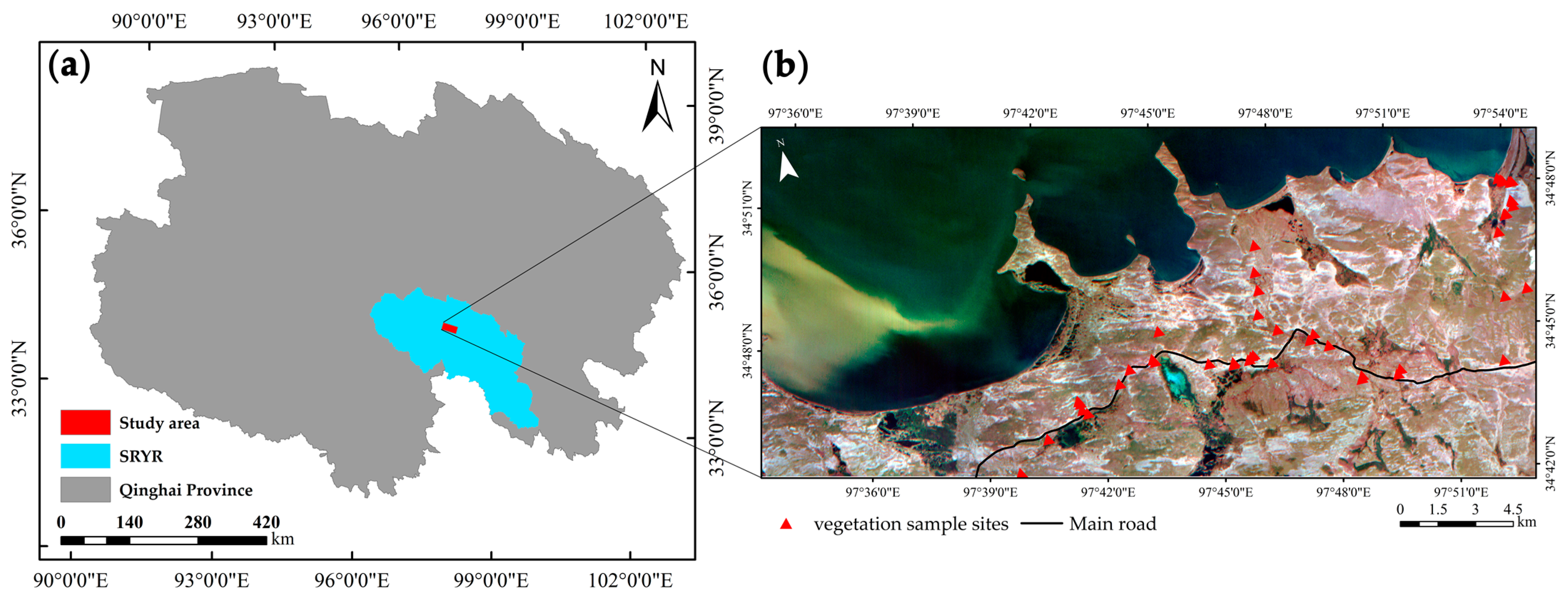
Figure 1. Schematic diagram of the study area. (a) Qinghai Province, China. (b) OHS-3C image (study area).
Remotesensing 15 03174 g001
Figure 2. HybridSN model structure diagram.
Remotesensing 15 03174 g002
Figure 3. HybridSN classification results in the study area. (a) Classification result from HJ-1A hyperspectral image in 2013. (b) Classification result from OHS-3C hyperspectral image in 2020.
Remotesensing 15 03174 g003
Figure 4. Vegetation classification verification results in 2020.
Remotesensing 15 03174 g004
Figure 5. GF-5 hyperspectral image classification result in 2019.
Remotesensing 15 03174 g005
Figure 6. The relationship between land objects and features between 2013 and 2020.
Remotesensing 15 03174 g006
Figure 7. Temperature and precipitation slope analysis results. (a) Surface temperature variation trend. (b) Annual precipitation variation trend.
Remotesensing 15 03174 g007
Figure 8. Noxious weed distribution area. (a) Noxious weed area across altitude–slope gradients. (b) Noxious weed distribution area at different altitudes in 2013 and 2020.
Remotesensing 15 03174 g008
Figure 9. Thermopsis lanceolata association distribution result.
Remotesensing 15 03174 g009
Figure 10. Thermopsis lanceolata association spatial pattern characteristics.
Remotesensing 15 03174 g010
Figure 11. NNH analysis of Thermopsis lanceolata association.
Remotesensing 15 03174 g011
Table 1. Information on hyperspectral remote sensing images.
NumberAcquisition DateSensorSatelliteNumber of BandsSpatial Resolution (m)
116 August 2013HSIHJ-1A115100
213 August 2019AHSIGF-533030
324 August 2020CMOSOHS-3C3210
Table 2. The typical field investigation vegetation types in the study area.
Vegetation TypesLongitude and LatitudePhotos
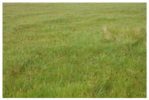
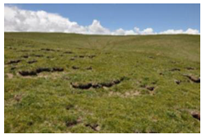
Carex moorcroftii, Kobresia tibetica Maxim cluster34°48’N, 97°53’ERemotesensing 15 03174 i001
Kobresia humilis, Leontopodium pusillum association34°45’N, 97°53’ERemotesensing 15 03174 i002
Kobresia humilis, Stipa
purpurea association
34°45’N, 97°46’ERemotesensing 15 03174 i003
Poa poophagorum, Stipa purpurea association34°45’N, 97°41’ERemotesensing 15 03174 i004
Stipa purpurea association34°47’N, 97°46’ERemotesensing 15 03174 i005
Stipa purpurea,
Leontopodium pusillum association
34°46’E, 97°46’NRemotesensing 15 03174 i006
Noxious weeds (Oxytropis ochrocephala Bunge in the picture)34°45’E, 97°45’NRemotesensing 15 03174 i007
Table 3. Study area vegetation association information.
Vegetation
Association
Dominant
Species
Subdominant SpeciesCompanion Species
Stipa purpurea associationStipa purpurea Elymus dahuricus Turcz, Roegneria thoroldiana, Kobresia humilis, etc.
Carex moorcroftii, Kobresia tibetica Maxim associationCarex moorcroftiiKobresia tibetica MaximScirpus distigmaticus,
Pteridophyta, Cremanthodium Benth, etc.
Kobresia humilis, Stipa purpurea associationKobresia humilisStipa purpureaPoa poophagorum,
Kobresia humilis,
Leontopodium pusillum, etc.
Poa poophagorum, Stipa purpurea associationPoa poophagorumStipa purpureaElymus dahuricus Turcz,
Kobresia humilis, etc.
Kobresia humilis, Leontopodium
pusillum association
Kobresia humilisLeontopodium
pusillum
Oxytropis, Stipa purpurea, Poa poophagorum, etc.
Stipa purpurea,
Leontopodium
pusillum association
Stipa purpureaLeontopodium
pusillum
Oxytropis, Ajania khartensis,
Poa poophagorum, etc.
Noxious weedsThermopsis lanceolate, Ligularia virgaurea, Aconitum pendulum, Oxytropis, Leontopodium pusillum, Saussurea japonica, Polygonum sibiricum Laxm, Ajania khartensis, Pedicularis kansuensis Maxim, etc.
Table 4. Training and test sample numbers in the study area.
CategoriesHJ-1AGF-5OHS-3C
Number of Training SamplesNumber of Testing SamplesNumbersof Training SamplesNumber of Testing SamplesNumber of Training SamplesNumber of Testing Samples
Lake410176758325816350
Bare ground1024416270729312
Noxious weeds1364820319137
Stipa purpurea association6729276118509218
Carex moorcroftii, Kobresia tibetica Maxim association873720688888380
Kobresia humilis, Stipa purpurea association8637223951165499
Poa poophagorum, Stipa purpurea association86372691151194512
Kobresia humilis, Leontopodium
pusillum association
1114713458792340
Stipa purpurea,
Leontopodium
pusillum association
9038263113869373
Total10524512339100272813121
Table 5. The UA and PA of each category.
CategoriesUA (%)PA (%)
HJ-1AGF-5OHS-3CHJ-1AGF-5OHS-3C
Noxious weeds83.33100.0097.46100.00100.0099.14
Lake99.7899.75100.00100.00100.00100.00
Bare ground100.00100.00100.0097.73100.00100.00
Carex moorcroftii, Kobresia tibetica Maxim association100.00100.0098.58100.0097.9899.71
Kobresia humilis, Leontopodium
pusillum association
100.00100.0098.04100.0098.8299.34
Kobresia humilis, Stipa purpurea
association
97.7197.35100.0098.46100.0099.33
Poa poophagorum, Stipa purpurea association98.9698.7999.4199.3199.1998.82
Stipa purpurea, Leontopodium
pusillum association
99.4299.3298.5597.1696.0896.88
Stipa purpurea association100.0096.4796.4499.0098.8098.19
Table 6. Area statistics of classification results in the study area.
Categories2013
(km2)
Proportion (%)2020
(km2)
Proportion (%)Growth Rate (%)
Lake20847.59%195.4444.71%−6.04%
Bare ground19.234.40%17.243.94%−10.35%
Noxious weeds2.880.66%9.022.06%213.19%
Stipa purpurea association28.626.55%14.73.36%−48.64%
Carex moorcroftii, Kobresia tibetica Maxim association20.724.74%24.135.52%16.46%
Poa poophagorum, Stipa purpurea association42.569.74%57.4213.14%34.92%
Kobresia humilis, Stipa purpurea association29.86.82%40.199.19%34.87%
Kobresia humilis, Leontopodium pusillum association57.4713.15%38.058.70%−33.79%
Stipa purpurea, Leontopodium pusillum association27.836.37%40.929.36%47.04%
Table 7. Comparison statistics of extraction results in 2019 and 2020.
CategoriesProportion in 2019 (%)Proportion in 2020 (%)Difference (%)
Lake27.82%25.81%2.01%
Bare ground4.55%3.10%1.45%
Noxious weeds1.65%1.41%0.24%
Stipa purpurea association7.14%8.62%−1.48%
Carex moorcroftii, Kobresia tibetica Maxim association6.82%3.80%3.02%
Poa poophagorum, Stipa purpurea
association
20.68%22.34%−1.66%
Kobresia humilis, Stipa purpurea association7.37%9.31%−1.94%
Kobresia humilis, Leontopodium
pusillum association
8.46%11.17%−2.71%
Stipa purpurea, Leontopodium
pusillum association
15.51%14.44%1.07%
Table 8. Transition matrix for 2013–2020/km2.
2013NWLakeBGCKKLKSPSSLSCTotal
2020
NW0.372.101.470.451.760.310.850.701.019.02
Lake0.09191.740.180.900.910.080.590.550.4195.44
BG0.140.434.350.284.770.680.842.922.8317.24
CK0.212.740.537.542.894.073.541.291.3224.13
KL0.360.965.080.6611.991.823.527.016.6538.05
KS0.621.581.793.838.4413.045.402.772.7240.19
PS0.784.101.924.6311.817.0017.954.534.7057.42
SL0.163.662.492.0310.551.967.895.886.3040.92
SC0.150.691.420.404.350.841.982.182.6914.70
Total2.88208.0019.2320.7257.4729.8042.5627.8328.62437.11
Remarks: Noxious weeds—NW; Lake—Lake, Bare Ground—BG; Carex moorcroftii, Kobresia tibetica Maxim association—CK; Kobresia humilis, Leontopodium pusillum association—KL; Kobresia humilis, Stipa purpurea association—KS; Poa poophagorum, Stipa purpurea association—PS; Stipa purpurea, Leontopodium pusillum association—SL; Stipa purpurea association—SC.
Table 9. The hierarchical list of slopes.
Scheme 0.0–77–25
GradeBottomlandGentle slope
Table 10. The hierarchical list of altitudes.
Altitude/m4200–42504250–43004300–43504350–44004400–44504450–45004500–4550
GradeIIIIIIIVVVIVII
Table 11. Zone A land cover change comparison in 2013 and 2020.
CategoriesArea in 2013 (km2)Area in 2020 (km2)Difference (km2)Growth Rate (%)
Water1.090.94−0.15−13.76
Herbaceous swamp1.000.69−0.31−31.00
Grass land29.6531.421.776.00
Bare ground3.251.94−1.31−40.31
Disclaimer/Publisher’s Note: The statements, opinions and data contained in all publications are solely those of the individual author(s) and contributor(s) and not of MDPI and/or the editor(s). MDPI and/or the editor(s) disclaim responsibility for any injury to people or property resulting from any ideas, methods, instructions or products referred to in the content.