Improved PPP-RTK by Considering the Non-Homogeneous Uncertainty of the ionosphere with a Spatial Three-Direction Model

Abstract

The ultimate goal of PPP-RTK is to achieve rapid ambiguity resolution, which is influenced by the prior precision of the external ionospheric information. This study proposes a method for determining the precision of ionospheric corrections for each satellite. In this method, an 8 min piece-wise function linearly related to the spatial three-direction distance components (SDC) within the geocentric coordinate system is constructed. By exploiting the SDC model, the user can calculate the precision of the ionospheric corrections satellite by satellite. Using the German and French stations, we validate this method experimentally and compare it to a method with an 8 min piece-wise function constructed by the baseline length (BLL). The SDC model provides an accuracy better than 10 mm in modeling ionospheric correction precision for each GPS satellite, with an average improvement of 43% compared to the BLL model. In addition, the SDC model offers an accuracy of approximately 5 mm in the reference network with an inter-station distance of less than 100 km, which is about 15% better than that of the BLL model during the active ionospheric period. The SDC model exhibits advantages over ionospheric correction precision modeling, with an average improvement of 73.5% for a reference network with station spacing of 125–155 km. By adopting the adaptive ionospheric precision derived from the SDC model, the GPS/GPS + Galileo PPP-RTK achieves a horizontal error of 50 mm and a vertical error of 100 mm within an average of three to four epochs. Notably, the convergence time is significantly enhanced by 30% in reference networks with inter-station distances of 125–155 km, compared to that of the PPP-RTK solution generated with dynamic ionospheric correction precision from the BLL model for all observed satellites.

1. Introduction

Precise point positioning (PPP) has been widely adopted in various fields, such as precision agriculture, seismology, and atmospheric science, owing to its high positioning accuracy, operational simplicity, and wide application range [1,2,3]. Unfortunately, the traditional float PPP requires 30 min or more to achieve centimeter-level positioning accuracy [4]. To date, a few strategies have been developed to speed up PPP convergence. One well-known route is introducing multi-GNSS uncalibrated phase delay products to assist in PPP ambiguity resolution (PPP-AR) [5,6]. Research has shown that multi-GNSS PPP-AR can be achieved with a convergence time of approximately 10 min [7]. Nevertheless, the convergence time of multi-GNSS PPP-AR is still unacceptable for real-time applications.

Compared to PPP, network-based real-time kinematic (NRTK) technology can achieve real-time and high-precision positioning services for the user station by using the differential correction generated by the reference station [8]. However, it is restricted by a baseline distance of less than 50 km [9]. Furthermore, a large amount of data broadcasting is another important limiting factor for NRTK [10]. To make the most of the advantages of both technologies and overcome their limitations, the concept of PPP-RTK was proposed and has been applied in recent years [11,12,13]. Different from NRTK, the PPP-RTK technology provides the user with individual undifferenced corrections, such as fractional phase bias, ionospheric delay, and tropospheric delay corrections generated from the reference network [14,15]. The undifferenced model can separate the various errors and broadcast them at different frequencies depending on the rate of variation of the errors, thus reducing the burden of real-time data communication [16]. Moreover, compared to the PPP-AR, the PPP-RTK makes rapid ambiguity resolution possible by providing precise undifferenced ionospheric correction [12]. However, the time to first fix (TTFF) is influenced by the a priori precision of the ionospheric corrections [17]. Related studies have demonstrated that TTFF can be significantly reduced if the a priori variances are best matched to the accuracy of the ionospheric corrections [18].

To achieve rapid ambiguity resolution, the users must appropriately determine the a priori precision of the high-accuracy ionospheric correction. Ionospheric corrections imported to directly correct ionospheric delay at the user station were treated as deterministic quantities [19,20]. This method has been demonstrated to be feasible for achieving instantaneous PPP-AR, but it is mainly applicable in reference networks with dense stations. Currently, the ionospheric corrections are often treated as random variables [21,22]. Empirical values for the standard deviations of ionospheric corrections are given according to the reference network scale, which can enhance the PPP-RTK positioning performance [23]. However, as the reference network scale changes, the given empirical values may not effectively reflect the spatial variation in the ionospheric delay. Wang et al. investigated the influence of the inter-station distance on the standard deviation of ionospheric correction [24]. The results demonstrate that the standard deviation value grows as the inter-station distance of the reference network increases. Considering the effect of the reference network scale on ionospheric correction accuracy, empirical linear or exponential functions related to the baseline length (BLL) have been employed to calculate the standard deviation value of ionospheric correction [25,26,27]. These standard deviation values will change with the station spacing of the reference network, but it may experience an accuracy degradation due to the overlooking of the temporal variation in the ionospheric delay. Most of the studies mentioned above were based on empirical models. High ionospheric activity and changes in the reference network size may cause biases in the empirical values based on the actual ionospheric delay accuracy. To obtain a more precise approximation of the actual precision, the standard deviation values of the ionospheric delay residuals were fitted in real time for all satellites using a linear function of the baseline length. The coefficients of the linear function were estimated using short-term observational data [28,29,30]. With coefficients either estimated in real-time or set to empirical values, a linear function of the baseline length is used as a traditional strategy for modeling the precision of ionospheric correction, described as the BLL model.

In the aforementioned studies, stochastic models for ionospheric correction were predominantly constructed based on ionospheric delay errors for all satellites. However, the precision of ionospheric delay differs for each satellite due to differences in the paths of satellite signals as they pass through the ionosphere [31], and spatial modeling of the ionospheric delay error RMS for a single satellite has rarely been investigated. Moreover, the ionosphere is not uniformly distributed, particularly during active ionospheric periods [32]. The BLL model, constructed by a linear and distance-dependent function, does not account for the variation in ionospheric delay precision in the three spatial directions, leading to reduced accuracy [33]. This study establishes an a priori stochastic model for ionospheric corrections based on the distance components in three spatial directions within the geocentric coordinate system. An 8 min piece-wise function is employed to model the ionospheric correction precision satellite by satellite. The fitting values of this model are utilized to weigh the ionospheric corrections at the user station, thereby enhancing the performance of the PPP-RTK positioning.

We first introduce the method for extracting the precise ionospheric delay, constraining ionospheric delay parameters at user stations, and constructing the stochastic model for ionospheric correction. Then, the PPP-RTK data processing strategy is presented. The observations of the stations distributed in France and the SAPOS network are introduced and used for ionospheric correction precision modeling and the PPP-RTK positioning tests. Finally, the fitting accuracy of the SDC model is compared with that of the BLL model, and the PPP-RTK positioning preformation with adaptive ionospheric precision derived from the SDC model is investigated and compared with that derived from the BLL model.

2. GNSS Observation Model

2.1. Extracting Precise Ionospheric Correction

The undifferenced and uncombined (UDUC) PPP observation equations for the pseudo-range and phase observations can be expressed as [34]:

$$\left\{\begin{array}{l}{P}_{r,j}^s={\rho }_r^s+c\cdot (t_r-t^s)+(d_{r,j}^{}-d_j^s)+C_j\cdot I_{r,j}^s+M^{}\cdot T_r^{}+e_{r,P}^s\\ L_{r,j}^s={\rho }_r^s+c\cdot (t_r-t^s)+{\lambda }_j^{}{N}_{r,j}^s+{\lambda }_j^{}(b_{r,j}^{}-b_j^s)-C_j\cdot I_{r,j}^s+M^{}\cdot T_r^{}+{\epsilon }_{r,L}^s\end{array}\right.$$

(1)

where $P_{r,j}^s$ and $L_{r,j}^s$ refer to the pseudo-range and phase observations, respectively, at the frequency ($j$ = 1, 2); ${\rho }_r^s$ denotes the geometric distance from the satellite to the receiver; $c$ is the speed of light in vacuum; $t_r^{}$ denotes the receiver clock offset; $t_{}^s$ is the satellite clock offset; ${\lambda }_j^{}$ is the wavelength of frequency $j$; $N_{r,j}^s$ is the integer ambiguity; $d_{r,j}^{}$ and $d_j^s$ are the pseudo-range code bias of the receiver and satellites, respectively; $b_{r,j}^{}$ and $b_j^s$ denote the carrier phase hardware delay of the receiver and satellites, respectively; $C_j^{}={\lambda }_j^2/{\lambda }_1^2$ is the ionospheric coefficient on frequency $j$; $I_{r,j}^s$ represents the first-order ionospheric delay; $M$ refers to the tropospheric mapping function; $T_r^{}$ represents the tropospheric zenith wet delay; $e_{r,P}^s$ and ${\epsilon }_{r,L}^s$ are the sum of unmodeled error and noise for pseudo-range and phase observation, respectively. Other system errors, such as solid earth tides, ocean tides, phase center offset (PCO), phase center variation (PCV), and relativistic effects, can be precisely corrected using existing models [35,36,37,38].

The parameters in the original observation equation cannot be estimated individually because of the rank deficiency resulting from the correlation of the parameters [13]. Therefore, reparameterization is necessary before estimation. The ionosphere-free combination of the pseudo-range hardware delay is contained in the GFZ satellite clock products [39]. Due to the correlation between the parameters, receiver clock offset, ionospheric delay, and ambiguity parameters will all absorb some of the pseudo-range hardware delay [40]. Furthermore, with a strong correlation between the phase hardware delay and the integer ambiguity parameter, the phase hardware delay at both the receiver and satellite ends is directly absorbed by ambiguity [41]. As a result, the re-parameterized equation can be expressed as follows [42]:

$$\left\{\begin{array}{cc}\hfill P_{r,j}^s=& {\mathsf{\rho }}_r^s+\left[\left(c·t_r+d_{r,IFr}\right)-\left(c·t^s+d_{,IF}^s\right)\right]+M·T_r\hfill \\ & +C_j·\left[I_{r,j}^s-\frac{f_2^2}{f_1^2-f_2^2}·\left(DC{B}_r-DC{B}^s\right)\right]+k·IS{B}_r^{G,SYs}+e_{r,P}^s\hfill \\ \hfill L_{r,j}^s=& {\mathsf{\rho }}_r^s+\left[\left(c·t_r+d_{r,IFr}\right)-\left(c·t^s+d_{,IF}^s\right)\right]+M·T_r\hfill \\ & +\left[{\lambda }_j·\left(N_j^s+b_{r,j}-b_j^s\right)+\left(d_{IF,r}-d_{IF}^s\right)-C_j·\frac{f_2^2}{f_1^2-f_2^2}·\left(DC{B}_r-DC{B}^s\right)\right]\hfill \\ & -C_j·\left[I_{r,j}^s-\frac{f_2^2}{f_1^2-f_2^2}·\left(DC{B}_r-DC{B}^s\right)\right]+{\epsilon }_{r,L}^s\hfill \end{array}\right.$$

(2)

Each of the estimated parameters can be expressed as follows:

$$k=\left\{\begin{array}{l}0\begin{array}{cc}& SYS=GPS\hfill \end{array}\\ 1\begin{array}{cc}& SYS=Galieo\hfill \end{array}\end{array}\right.$$

(3)

$$\left\{\begin{array}{c}{\overline{t}}^s=c·t^s+d_{,IF}^s\hfill \\ {\overline{t}}_r=c·t_r+d_{r,IF}\hfill \\ d_{r,IF}=\frac{f_1^2}{f_1^2-f_2^2}·d_{r,1}-\frac{f_2^2}{f_1^2-f_2^2}·d_{r,2}\hfill \\ d_{,IF}^s=\frac{f_1^2}{f_1^2-f_2^2}·d_{,1}^s-\frac{f_2^2}{f_1^2-f_2^2}·d_{,2}^s\hfill \\ DC{B}_r=d_{r,1}-d_{r,2}\hfill \\ DC{B}^s=d_{,1}^s-d_{,2}^s\hfill \\ d_{r,1}=d_{r,IF}-\frac{f_2^2}{f_1^2-f_2^2}·DC{B}_r\hfill \\ d_{,1}^s=d_{,IF}^s-\frac{f_2^2}{f_1^2-f_2^2}·DC{B}^s\hfill \\ {\overline{I}}_{r,j}^s=I_{r,j}^s-\frac{f_2^2}{f_1^2-f_2^2}·\left(DC{B}_r-DC{B}^s\right)(j=1)\hfill \\ {\overline{N}}_j^s=\left(N_j^s+b_{r,j}-b_j^s\right)+\left[\left(d_{IF,r}-d_{IF}^s\right)-C_j·\frac{f_2^2}{f_1^2-f_2^2}·\left(DC{B}_r-DC{B}^s\right)\right]/{\lambda }_j\hfill \end{array}\right.$$

(4)

where ${\overline{t}}_r^{}$ denotes the receiver clock offset that absorbs the pseudo-range hardware delay at the receiver end; ${\overline{t}}_{}^s$ refers to the satellite clock offset that absorbs the pseudo-range hardware delay at the satellite end [43], which is no longer estimated as a parameter and can be corrected directly using the precise product; $DC{B}_{}^s$ and $DC{B}_r^{}$ are the differential code bias ($DCB$) at the satellite and receiver ends, respectively; ${\overline{I}}_{r,j}^s$ is the ionospheric delay parameter that absorbs the differential code bias of the receiver and the satellite end [44]. $IS{B}_r^{G,SYS}$ denotes the inter-system bias ($ISB$) parameter between the satellite system $SYS$ and GPS, and the value for the GPS satellite is 0 [45]; ${\overline{N}}_{r,j}^s$ is the float ambiguity at the frequency ($j$ = 1, 2), which no longer exhibits integer characteristics owing to the absorption of hardware delays at the satellite and receiver ends [46]. As a result, the pseudo-range and phase observation equations can be simplified as follows:

$$\left\{\begin{array}{l}{P}_{r,j}^s={\mathsf{\rho }}_r^s+({\overline{t}}_r-{\overline{t}}^s)+T_r^G+C_j^{}\cdot {\overline{I}}_{r,j}^s+k\cdot IS{B}_r^{G,S\mathrm{Y}S}+e_{r,P}^s\\ L_{r,j}^s={\mathsf{\rho }}_r^s+({\overline{t}}_r-{\overline{t}}^s)+{\lambda }_j^{}{\overline{N}}_{r,j}^{s,}+M\cdot T_r^{}-C_j^{}\cdot {\overline{I}}_{r,j}^s+{\epsilon }_{r,L}^s\end{array}\right.$$

(5)

To improve the accuracy of the extracted slant ionospheric delay, we achieve PPP-AR on the reference stations with fixed station coordinates and employ a partial ambiguity resolution (PAR) strategy [47]. After successful ambiguity resolution, ionospheric corrections are derived from the slant ionospheric delay extracted from the reference stations and broadcast to the user station.

2.2. Constraining Ionospheric Delay Parameters at User Stations

The receiver DCB of the reference stations is contained in ionospheric corrections derived from the reference network, which are unknown to the user station. It is impossible to use the undifferenced correction to constrain the PPP solution for a user. To eliminate the effect of receiver DCB, single-difference-between-satellite (SDBS) ionospheric correction is imported as virtual observation by selecting the satellite with the maximum product of the elevation angle and observation time as the reference satellite [48]. After introducing virtual observation, the UDUC PPP observation equation can be expressed as follows [42]:

$$\left\{\begin{array}{l}{P}_{r,j}^s={\mathbf{u}}_{\mathbf{r}}^{\mathbf{s}}\cdot \mathsf{\Delta }\mathbf{x}+c({\overline{t}}_u-{\overline{t}}^s)+T_u^{}+C_j^{}\cdot {\overline{I}}_u^s+e_{u,P}^s\\ L_{r,j}^s={\mathbf{u}}_{\mathbf{r}}^{\mathbf{s}}\cdot \mathsf{\Delta }\mathbf{x}+c({\overline{t}}_u-{\overline{t}}^s)+{\lambda }_j^{}{\overline{N}}_{u,j}^{s,}+M\cdot T_u^{}-C_j^{}\cdot {\overline{I}}_u^s+{\epsilon }_{u,L}^s\\ {\overline{I}}_{}^{s,s_0^{}}-({\overline{I}}_u^s-{\overline{I}}_u^{s_0^{}})=w_{\overline{I}}^{},w_{\overline{I}}^{}\sim N(0,{\sigma }_{\overline{I}}^2)\end{array}\right.$$

(6)

where $S_0^{}$ is the reference satellite; ${\overline{I}}_{}^{s,s_0^{}}$ denotes the ionospheric virtual observation; $\mathsf{\Delta }\mathbf{x}$ is the amount of change in the receiver coordinates relative to the initial position in the user station; ${\mathbf{u}}_{\mathbf{r}}^{\mathbf{s}}$ refers to the direction cosine vector from receiver to satellite; $w_{\overline{I}}^{}$ is the difference between (SDBS) ionospheric virtual observations and the true value of the SDBS ionospheric delay at the user station, with a mean value of 0 and a standard deviation value of ${\sigma }_{\overline{I}}^{}$.

To properly determine the precision of SDBS ionospheric correction, it is crucial for rapid ambiguity resolution at the user station [49]. In this study, a more accurate stochastic model for the ionospheric correction is constructed to describe the stochastic characteristics of SDBS ionospheric corrections and determine their precision.

3. Constructing the Stochastic Model for Ionospheric Correction

To date, different methods for interpolating ionospheric correction have been proposed, such as the linear combination method (LCM), the linear interpolation method (LIM), and the inverse squared distance weighting algorithm (IDW) [39]. Research has shown that the performance of these methods is comparable [50]. Therefore, we use an inverse squared distance weighting algorithm to interpolate the ionospheric correction [51]. The interpolation is performed as follows:

$$\begin{array}{cc}{\overline{I}}_{}^{s,s_0^{}}={\displaystyle {\sum }_{r=1}^3{A}_r^{}{\overline{I}}_r^{s,s_0^{}}}& A_r^{}=\frac{\frac{1}{d_r^2}}{{\displaystyle {\sum }_{r=1}^3\frac{1}{d_r^2}}}\end{array}$$

(7)

where $d_r^{}$ refers to the baseline length from reference station $r$ to user station $u$; $A_r^{}$ is the weight of the ionospheric virtual observation from each reference station.

This study aimed to determine the a priori precision of the SDBS ionospheric delay interpolation generated by different reference networks, from near to far. Therefore, the standard deviation values that depend on the reference network scale are studied. Each reference network constructed by stations adjacent to the user is equivalent to a virtual station. The baseline length from the user to the virtual station is denoted by $d_{}^{}$, and the SDBS ionospheric delay from the virtual station is represented by ${\overline{I}}_{}^{s,s_0^{}}$. The station-satellite-double-difference (SSDD) ionospheric delay can be analyzed as a function of the baseline lengths between the receivers [52]. The difference between ${\overline{I}}_{}^{s,s_0^{}}$ and ${\overline{I}}_u^{s,s_0^{}}$ is expressed as:

$$\mathsf{\Delta }{\overline{I}}_{v,u}^{s,s_0^{}}={\overline{I}}_{}^{s,s_0^{}}-{\overline{I}}_u^{s,s_0^{}}=f(I)\cdot d_{}^{}$$

(8)

where $\mathsf{\Delta }{\overline{I}}_{v,u}^{s,s_0^{}}$ is the station-satellite-double-difference (SSDD) ionospheric delay; $v$ denotes the virtual station; $f(I)$ represents the residual of the ionospheric correction for a baseline length of 1 km. The value of $STD(f(I))$ can be regarded as the constant value and be utilized directly to compute the precision of the ionospheric correction in the geocentric coordinate system. The standard deviation of SSDD ionospheric delay is:

$$\begin{array}{l}STD(\mathsf{\Delta }{\overline{I}}_{v,u}^{s,s_0^{}})=STD({\overline{I}}_{}^{s,s_0^{}}-{\overline{I}}_u^{s,s_0^{}})\\ \begin{array}{ccc}\begin{array}{cc}& \end{array}& & \end{array}=STD({\overline{I}}_u^{s,s_0^{}}-{\displaystyle {\sum }_{r=1}^3{A}_r^{}{\overline{I}}_r^{s,s_0^{}}})\\ \begin{array}{ccc}\begin{array}{cc}& \end{array}& & \end{array}=STD(f(I)\cdot d_{}^{})\end{array}$$

(9)

The standard deviation value of SSDD ionospheric delay can be modeled by a function linearly related to the baseline length, as in the following equation:

$$\begin{array}{l}STD(\mathsf{\Delta }{\overline{I}}_{v,u}^{s,s_0^{}})=STD({10}_{}^{-3}\cdot f(I))\cdot d_{}^{}\\ \begin{array}{ccc}\begin{array}{cc}& \end{array}& & \end{array}=a\cdot d\end{array}$$

(10)

where $a$ is the coefficient of the BLL model, which can be fixed or estimated in real time.

Since the ionosphere is an inhomogeneous medium, spatial gradients are usually present [52]. We perform a Taylor expansion for the baseline length in the geocentric coordinate system. The Taylor expansion for the baseline length $d$ is expressed as:

$$\begin{array}{cc}\hfill d=& \sqrt{{\left(\mathsf{\Delta }{x}_{vu}\right)}^2+{\left(\mathsf{\Delta }{y}_{vu}\right)}^2+{\left(\mathsf{\Delta }{z}_{vu}\right)}^2}\hfill \\ & =f\left(\mathsf{\Delta }{x}_{vu},\mathsf{\Delta }{y}_{vu},\mathsf{\Delta }{z}_{vu}\right)\hfill \\ & =\sqrt{{\left(\mathsf{\Delta }{x}_0\right)}^2+{\left(\mathsf{\Delta }{y}_0\right)}^2+{\left(\mathsf{\Delta }{z}_0\right)}^2}\hfill \\ & +\frac{\mathsf{\Delta }{x}_0}{\sqrt{{\left(\mathsf{\Delta }{x}_0\right)}^2+{\left(\mathsf{\Delta }{y}_0\right)}^2+{\left(\mathsf{\Delta }{z}_0\right)}^2}}\mathsf{\Delta }{x}_{vu}\hfill \\ & +\frac{\mathsf{\Delta }{y}_0}{\sqrt{{\left(\mathsf{\Delta }{x}_0\right)}^2+{\left(\mathsf{\Delta }{y}_0\right)}^2+{\left(\mathsf{\Delta }{z}_0\right)}^2}}\mathsf{\Delta }{y}_{vu}\hfill \\ & +\frac{\mathsf{\Delta }{z}_0}{\sqrt{{\left(\mathsf{\Delta }{x}_0\right)}^2+{\left(\mathsf{\Delta }{y}_0\right)}^2+{\left(\mathsf{\Delta }{z}_0\right)}^2}}\mathsf{\Delta }{h}_{vu}+o\hfill \\ \hfill \approx & \alpha ·\mathsf{\Delta }{x}_{vu}+\beta ·\mathsf{\Delta }{y}_{vu}+\gamma ·\mathsf{\Delta }{z}_{vu}+C\hfill \end{array}$$

(11)

$$\begin{array}{l}\alpha =\frac{\mathsf{\Delta }{x}_0^{}}{\sqrt{{(\mathsf{\Delta }{x}_0^{})}_{}^2+{(\mathsf{\Delta }{y}_0^{})}_{}^2+{(\mathsf{\Delta }{z}_0^{})}_{}^2}}\\ \beta =\frac{\mathsf{\Delta }{y}_0^{}}{\sqrt{{(\mathsf{\Delta }{x}_0^{})}_{}^2+{(\mathsf{\Delta }{y}_0^{})}_{}^2+{(\mathsf{\Delta }{z}_0^{})}_{}^2}}\\ \gamma =\frac{\mathsf{\Delta }{z}_0^{}}{\sqrt{{(\mathsf{\Delta }{x}_0^{})}_{}^2+{(\mathsf{\Delta }{y}_0^{})}_{}^2+{(\mathsf{\Delta }{z}_0^{})}_{}^2}}\\ C=\sqrt{{(\mathsf{\Delta }{x}_0^{})}_{}^2+{(\mathsf{\Delta }{y}_0^{})}_{}^2+{(\mathsf{\Delta }{z}_0^{})}_{}^2}\end{array}$$

(12)

where $\mathsf{\Delta }{x}_{vu}^{}$, $\mathsf{\Delta }{y}_{vu}^{}$, and $\mathsf{\Delta }{z}_{vu}^{}$ are the difference in spatial coordinates between the user station and the virtual station; $\mathsf{\Delta }{x}_0^{}$, $\mathsf{\Delta }{y}_0^{}$, and $\mathsf{\Delta }{z}_0^{}$ are the initial values of the Taylor expansion. By substituting Equation (11) into Equation (9), we obtain Equation (13):

$$STD(\mathsf{\Delta }{\overline{I}}_{v,u}^{s,s_0^{}})\approx c_1^{}\cdot \mathsf{\Delta }{x}_{vu}^{}+c_2^{}\cdot \mathsf{\Delta }{y}_{vu}^{}+c_3^{}\cdot \mathsf{\Delta }{z}_{vu}^{}+c_0^{}$$

(13)

$$\begin{array}{l}\mathsf{\Delta }{x}_{vu}^{}={\displaystyle {\sum }_{r=1}^3{A}_r^{}}\mathsf{\Delta }{x}_{ru}^{}\\ \mathsf{\Delta }{y}_{vu}^{}={\displaystyle {\sum }_{r=1}^3{A}_r^{}}\mathsf{\Delta }{y}_{ru}^{}\\ \mathsf{\Delta }{z}_{vu}^{}={\displaystyle {\sum }_{r=1}^3{A}_r^{}}\mathsf{\Delta }{z}_{ru}^{}\end{array}$$

(14)

where $\mathsf{\Delta }{x}_{ru}^{}$, $\mathsf{\Delta }{y}_{ru}^{}$, and $\mathsf{\Delta }{z}_{ru}^{}$ are the distances in the three spatial directions between the reference station $r$ and the user station $u$ within the geocentric coordinate system. To construct an accurate stochastic model, an observation equation is formed based on Equation (13), where the parameters $c_0^{}$, $c_1^{}$, $c_2^{}$, and $c_3^{}$ are estimated in real time using the least squares algorithm.

4. Results and Analysis

4.1. Experimental Setup and Processing Strategy

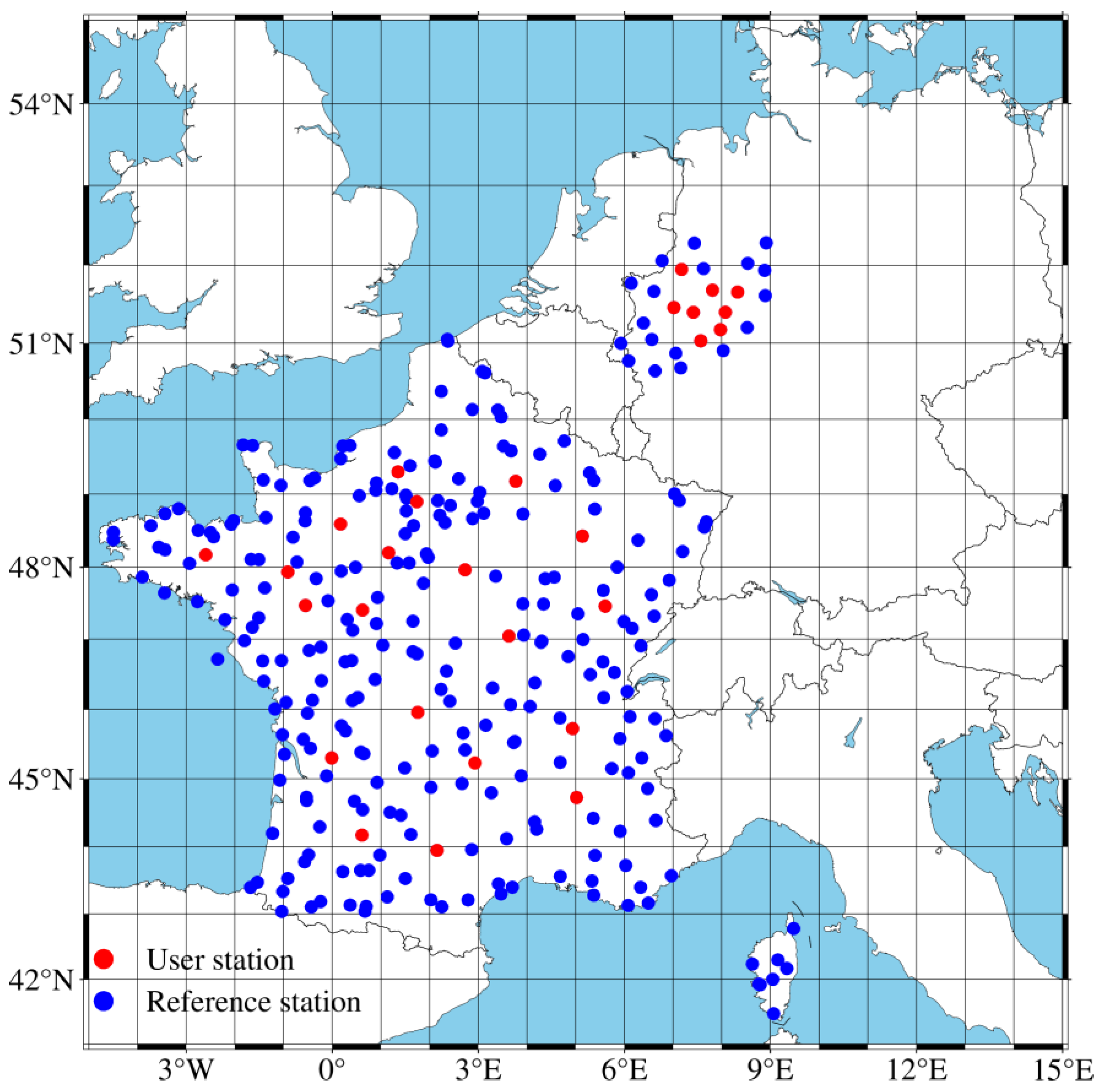
To evaluate the accuracy of the SDC and BLL models in reference networks with different inter-station distances, we analyzed the observation data for the 72-hour interval from DOY 276 to 278 in 2021 at 230 stations evenly distributed in France and Germany. The station distribution is shown in Figure 1, with solid blue circles denoting reference stations and red circles denoting user stations. With 28 stations serving as user stations (20 in France and 8 in Germany), the SDC and BLL models are constructed in eight different inter-station reference networks surrounding each user station. For each user station, the baseline length between the reference station and the user is calculated, and the stations are sorted in ascending order based on the baseline length. The three nearest reference stations are selected from the sorted results of reference stations to form the first reference network. The station with the longest baseline length in the first reference network is combined with the following two stations to form the second reference network. Similarly, the third reference network is constructed. The method of constructing reference networks with different station spacing around the user station is shown in Figure 2. Ultimately, eight reference networks are built around each of the 20 user stations, with inter-station distances of about 30, 60, 70, 80, 90, 120, 130, and 150 km, respectively. The inter-station distance is available by calculating the average baseline distance from a user station to all reference stations in a reference network.

The precision of the ionospheric correction is not related to the satellite system. This proposed method is applicable not only to GPS and Galileo but also to BDS and GLONASS. Owing to the numerous and evenly distributed stations in France, we adopt observations obtained from the French stations to assess the accuracy of the SDC and BLL models. With the lack of BDS, Galileo, and GLONASS observations at French stations, GPS observations with a sampling rate of 30 s are exclusively available at French stations and are used for GPS-only PPP-RTK positioning solutions. In addition, due to the few BDS and GLONASS observations available from the German station, GPS and Galileo observations with a sampling rate of 15 s are obtained from the SAPOS Network in Germany. GPS/GPS + Galileo PPP-RTK positioning solutions were obtained using observational data from German user stations. The data processing strategy for PPP-RTK is presented in

Table 1. The PPP-RTK data processing strategy.

Item	Strategies
Satellite system/frequency	GPS: L1/L2; Galileo: E1/E5a
Elevation cutoff angles	10°
Satellite orbits/clock offset	Corrected by the GBM precise orbit/integer clock product
Satellite antenna PCO/PCV	Corrected by igs14_2136.atx
Receive antenna PCO/PCV	Corrected by igs14_2136.atx
Tropospheric delay	Zenith hydrostatic delay: a priori value provided by the Saastamonien Model [53]
	Zenith wet delay: estimated as random-walk noise;
Ionospheric delay	Reference station: estimated as random-walk noise;
	User station: constrained by the ionospheric corrections;
Receiver coordinate	Reference station: fixed
	User station: estimated as white noise
Receiver clock	Estimated as white noise
Ambiguity	PAR
Area	Germany, France

.

4.2. Analysis of Ionospheric Correction Precision Modeling

After successful ambiguity resolution, the accurate ionospheric delays of the user and reference stations are extracted. Ionospheric delay residuals are calculated by subtracting the ionospheric delay interpolation from the ionospheric delay derived from the user station.

The RMS values of the ionospheric delay residuals, which are statistically calculated at 1-, 8-, and 30-min intervals, are presented in Figure 3. The RMS values computed at each time interval exhibit temporal variation. Notably, the RMS values at 1-min intervals can accurately capture the fine changes in ionospheric delays. Therefore, we employ the RMS values calculated at 1-min intervals as the reference values and analyze the RMS values at 8- and 30-min intervals. The RMS values at 30-min intervals change gradually with time, providing an overall outline of the ionospheric delay variation but failing to capture temporal-specific details. Conversely, the RMS values at 8-min intervals accurately capture the complex variability of the ionospheric delay over an 8-min duration and reduce the computational burden. Therefore, we employed 8-min intervals to model the ionospheric delay error RMS.

Without considering the variation in ionospheric delay precision in the three spatial directions, the BLL model is constructed with a simple function of the baseline distance and is widely used to model the precision of the ionospheric correction [23,24,25,26,27,28]. The coefficients of the SDC and BLL models are estimated separately using the RMS values of the ionospheric correction residuals every 8 min in each of the eight reference networks. With the estimated coefficients, the precision of ionospheric delay interpolation is modeled by the BLL and the SDC models in each of eight different references. Figure 4 shows the actual RMS values of the ionospheric delay interpolation errors and their corresponding fitting values of the SDC and BLL models in reference networks with different inter-station distances. The true values in Figure 4 are the actual RMS values of the ionospheric correction residuals for each 8 min duration in each of the eight reference networks. The RMS values for G05/G02 generally increase with the inter-station distance. The difference between the fitting value of the BLL model and the actual precision is no more than 5 mm within tens of kilometers, while it increases to 7.5 mm for G05 and 17 mm for G02 after the inter-station distance increases to 125–155 km. In contrast, the fitting errors of the SDC model do not exceed 3 mm over eight different inter-station distances. This indicates that the fitting values of the SDC model are in excellent agreement with the actual precision of the ionospheric corrections. Additionally, the mean values of the fitting errors of the SDC model for G05/G02 in reference networks with different inter-station distances are 1.3 mm, which is 65.8% and 81.2% higher than that of the BLL model, respectively. The results demonstrate that the fitting accuracy of the SDC model is superior to that of the BLL model.

To further evaluate the fitting accuracy of both models between the satellites, we obtained the fitting accuracy of the two models for each GPS satellite by calculating the RMS of the fitting errors of the two models in 160 reference networks and 20 user stations. The RMS values of the fitting error for each GPS satellite are shown in Figure 5. Notably, the fitting accuracy of the SDC model is better than that of the BLL model for each GPS satellite, with an average improvement of 43%. The RMS values for the BLL model exhibit fluctuations across different satellites, ranging from 1 mm to 20 mm. However, the fitting accuracy of the SDC model is better than 10 mm, and more than 80% of the satellites are better than 5 mm, which shows less variation among satellites compared with the BLL model. This indicates that the SDC model can provide high and stable fitting accuracy for different satellites.

Similar to GPS satellites, the fitting accuracy of the two models for each Galileo satellite is obtained by calculating the fitting error of the two models in eight reference networks in Germany. In comparison with GPS, Galileo reached similar conclusions. The fitting accuracy of the SDC model is better than the BLL model for each Galileo satellite, and the RMS values for the BLL model less than 10 mm exhibit better stability.

Figure 6 illustrates the results of the inter-satellite comparison of the SDC model coefficients C1, C2, and C3 in Equation (13). Our analysis reveals that the temporal variability of the model coefficients displays irregular and nonsynchronous characteristics for each satellite. These findings suggest that the coefficients of the SDC model are time-varying and differ between satellites. Furthermore, differences in any of the model coefficients of C1, C2, and C3 exist between the satellites, which are primarily attributed to differences in the ionospheric delay precision between satellites.

The afternoon period between 13:00–16:00 local time (LT) is considered to be an active ionosphere period [54]. In the reference network with an inter-station distance of 34 km, the fitting errors of the SDC and BLL models are calculated separately for each 8 min duration during calm (00:00–04:00 LT) and active ionospheric periods (13:00–16:00 LT). The results for G05 are presented as an example in Figure 7, where the solid orange and blue dots represent the fitting errors of the BLL model and SDC, respectively, in each 8 min duration. The fitting errors of both models exhibit irregular variations during the calm and active ionospheric periods but with similar trends. During the calm periods, the fitting errors of the two models are relatively close and remain below 4 mm for more than 80% of the observed periods. During the active ionospheric period, the fitting error of the SDC model is smaller than that of the BLL model and exhibits relatively stable variations, remaining below 4 mm for about 80% of the observed periods.

With observations from the 20 user stations and their surrounding 160 reference networks in France, we can obtain the fitting accuracy of the SDC and BLL models by calculating the RMS of the fitting error at each 8-min interval during a calm or active ionospheric period. Figure 8 displays the fitting accuracy of both models for different periods at each inter-station distance, using G05 as an example. For reference networks with inter-station distances of less than 100 km, the fitting accuracy of the SDC model during ionospheric calm periods is comparable to that of the BLL model, with both models providing an accuracy better than 5 mm. During the active ionospheric period, the fitting accuracy of the SDC model is maintained at approximately 5 mm, which is approximately 15% better than that of the BLL model. With inter-station distances increasing to 125–155 km, the fitting accuracy of the BLL model decreases significantly, exceeding 10 mm during the active ionospheric period and reaching 15 mm in reference networks with an inter-station distance of 155 km. In contrast, the SDC model shows better stability with a fitting accuracy of approximately 5 mm during calm and active ionospheric periods. The average improvement in fitting accuracy is 73.5% compared with the BLL model.

4.3. Analysis of Ionosphere-Weighted PPP-RTK Positioning Performance

To determine the a priori precision of the ionospheric corrections, the RMS values of the ionospheric correction errors for all satellites are usually fitted using a baseline distance [28,29,30]. The model coefficients are estimated using least squares or are set using empirical values. This study proposes four processing schemes, namely: (a) the coefficients of the BLL model are 0.74 mm/km and 1.04 mm/km in the calm and active ionospheric periods, respectively [55,56]; (b) the SDC model coefficients are estimated satellite-by-satellite every 8 min using least squares; (c) the coefficients of the BLL model are the same for all satellites and estimated every 8 min using the least squares algorithm; (d) the coefficients of the BLL model are estimated satellite-by-satellite every 8 min using the least squares algorithm. The PPP-RTK solution can be generated with the four ionosphere weighting strategies, namely, the calculated empirical value of scheme (a), the automatically calculated value of scheme (b), scheme (c), and scheme (d). They are simplified to “BLL-EXP”, “SDC-each-auto”, “BLL-all-auto”, and “BLL-each-auto” for the four schemes, and the PPP-RTK positioning tests are conducted at the French and German user stations.

Figure 9 and Figure 10 show the PPP-RTK positioning results for the French user station (PLGN) and German user station (2600) in the reference networks with inter-station distances of 52 km (PLGN) and 91 km (2600), respectively. The convergence is determined by horizontal positioning errors of less than 50 mm and vertical errors of less than 100 mm, with all satellite ambiguities initialized every 20 min. Among the four GPS-only PPP-RTK solutions, “G-BLL-EXP” exhibits the slowest convergence speed, with an average of 4.6 epochs for horizontal convergence and 4.2 epochs for vertical convergence. After the adaptive adjustment of the precision of the ionospheric delays, the average convergence time of “G-BLL-all-auto” and “G-BLL-each-auto” in the horizontal and vertical directions is reduced to 3.1 and 2.9 epochs, respectively. The “G-SDC-each-auto” algorithm achieves the fastest convergence speed, with an average of 2.6 epochs for horizontal convergence and 2.4 epochs for vertical convergence. This is primarily attributed to the fact that “G-SDC-each-auto” considers the variations of ionospheric delay accuracy for each satellite in three spatial directions.

In comparison with the GPS-only PPP-RTK, the GPS + Galileo PPP-RTK reaches similar conclusions. “GE-SDC-each-auto” achieves the fastest convergence speed. The convergence speed of “G-BLL-each-auto” is faster than that of “G-BLL-all-auto”, meaning that modeling the precision of the ionospheric correction for each satellite can improve the convergence performance of PPP-RTK. While “GE-BLL-EXP” converges at the slowest speed. Compared to “GE-SDC-each-auto”, the convergence time of “GE-BLL-EXP” increases by an average of 3.7 epochs.

In this study, we further investigate the convergence time, TTFF, and post-convergence positioning accuracy of three ionosphere-weighted PPP-RTK solutions at 28 user stations.

Figure 11 shows the convergence time of the GPS-only PPP-RTK in the horizontal and vertical directions for 20 user stations in France. The convergence performance of “G-SDC-each-auto” is the best among the four GPS-only PPP-RTK solutions. The convergence time of “G-SDC-each-auto” is slightly lower than “G-BLL-each-auto” and “G-BLL-all-auto” in the reference network, with an inter-station distance of 40~92 km. As the inter-station distance increases to 127–155 km, the “G-SDC-each-auto” demonstrates significant advantages in accelerating convergence, saving about 3.0, 2.0, and 1.0 epochs in convergence time compared to the “G-BLL-EXP”, “G-BLL-all-auto”, and “G-BLL-each-auto”, respectively. “G-BLL-all-auto” converges within four epochs in the reference networks with inter-station distances of 40–92 km, owing to the high accuracy of the BLL model at short inter-station distances. However, as the inter-station distance increases to 127–155 km, the epochs required for the convergence of “G-BLL-all-auto” in the horizontal and vertical directions are 6.9 and 6.6, respectively. These values are close to the 7.8 and 7.6 epochs required for “G-BLL-EXP” in the horizontal and vertical directions, respectively, primarily due to the relatively larger errors of the BLL model, resulting in slower convergence speed.

Figure 12 illustrates the convergence time of the GPS-only/GPS + Galileo PPP-RTK at eight user stations in Germany in both the horizontal and vertical directions. Similar to the French user station, the three GPS-only PPP-RTK solutions for the German user stations demonstrate comparable conclusions, albeit with slightly longer convergence times owing to differences in observation conditions. After adding Galileo observations, “GE-SDC-each-auto” exhibits the best convergence performance, with convergence times of 3.0 and 2.4 epochs in the horizontal and vertical directions, respectively. While “GE-BLL-EXP” converges at the slowest speed. For reference networks with inter-station distances of 40–70 km and 73–91 km, the convergence time of “GE-SDC-each-auto” is slightly lower than that of “GE-BLL-auto” and almost equal to that of “GE-BLL-each-auto”, with a reduction in approximately 1.8 epochs in the horizontal direction compared to “GE-BLL-EXP”. As the inter-station distance increases to 127–155 km, the convergence performance of “GE-SDC-auto” is significantly improved, with an increase of 36.9%, 29.3%, and 12.1% in the horizontal direction compared to “GE-BLL-EXP”, “GE-BLL-all-auto”, and “GE-BLL-each-auto”, respectively.

The conclusion drawn from GPS-only/GPS + Galileo PPP-RTK solutions is that “SDC-each-auto” demonstrates the best convergence performance in reference networks with inter-station distances of less than 155 km. In reference networks with inter-station distances of 127–155 km, “SDC-each-auto” exhibits a significant improvement of approximately 38%, 30%, and 12% compared to “BLL-EXP”, “BLL-all-auto”, and “BLL-each-auto”. “BLL-each-auto” exhibits rapid convergence in reference networks with short inter-station distances. However, the convergence performance of “BLL-all-auto” deteriorates in reference networks with larger station spacing as the fitting error of the BLL model increases.

Table 2. The positioning accuracy after convergence and mean TTFF of the GPS-only (France), GPS-only (Germany), and GPS + Galileo (Germany) PPP-RTK solutions for the 8 h sessions of the 28 user stations.

	GPS-Only (France)/GPS-Only (Germany)/GPS + Galileo (Germany)
	Overall Mean RMS: (unit: mm)			Mean TTFF (Epoch)
	E	N	U
BLL-EXP	8.6/9.4/5.4	7.6/8.4/5.1	22.3/22.4/21.5	5.6/6.7/4.3
BLL-all-auto	7.4/8.6/5.7	7.1/8.4/4.4	22.2/22.3/20.7	4.2/5.5/3.5
BLL-each-auto	7.9/8.1/5.7	7.0/7.9/4.2	22.1/20.6/18.8	3.9/4.9/3.2
SDC-each-auto	8.2/7.9/5.5	6.8/7.7/4.2	22.0/20.2/18.5	3.4/4.5/3.0

presents the mean TTFF and positioning accuracy after convergence for the GPS/GPS + Galileo PPP-RTK at the 28 user stations in France and Germany. After adjusting the precision of ionospheric corrections adaptively, the mean TTFF for the German and French stations decreases from 5.6 and 6.7 epochs for “G-BLL-EXP” to 4.2 and 5.5 epochs for “G-BLL-all-auto”, respectively. Furthermore, “G-SDC-each-auto”, which accounts for variations in ionospheric delay accuracy across three spatial directions for each satellite, further reduces the mean TTFF to 3.4 and 4.5 epochs, with a 39.2% and 32.8% improvement over “G-BLL-all-EXP”. The four GPS-only PPP-RTK solutions exhibit comparable positioning accuracy, ranging from 6.8 to 9.4 mm in the horizontal direction and 20 to 22 mm in the vertical direction, primarily due to the stabilization of ionospheric delay residuals after successful ambiguity resolution. With the addition of GPS + Galileo observations, the mean TTFF for “GE-SDC-each-auto” is reduced to 3.0 epochs, with a 14.2% and 31.8% improvement over “GE-BLL-all-auto” and “GE-BLL-EXP”, respectively. Furthermore, the four GPS + Galileo PPP-RTK solutions demonstrated improved positioning accuracy compared to the corresponding GPS-only PPP-RTK solutions, with a horizontal accuracy ranging from 4.2 to 5.7 mm and a vertical accuracy ranging from 18.5 to 21.5 mm.

5. Conclusions

The accurate determination of a priori precision for ionospheric corrections is essential for achieving rapid ambiguity resolution at the user station. We propose a method for determining the a priori precision of ionospheric correction for each satellite. In this method, an 8 min piece-wise function related to the spatial three-direction distance component is built to model the ionosphere correction error RMS satellite-by-satellite. With this method, higher modeling accuracy and better positioning performance of PPP-RTK can be achieved at the user station compared with a method using the BLL model.

This method is validated using observations from more than 230 stations in France and Germany, and the modeling accuracy of different satellites and station spacing within 155 km is investigated. The SDC model exhibits higher fitting accuracy than the BLL model for each GPS satellite, with relatively minor differences between the satellites. Both models demonstrate high accuracy during calm ionospheric periods for reference networks with inter-station distances of less than 100 km. However, during the active period, the SDC model improves the modeling accuracy by approximately 15% compared with the BLL model. As the inter-station distance increases to 125–155 km, the fitting accuracy of the BLL model significantly decreases. In contrast, the SDC model maintains an accuracy of approximately 5 mm during both periods, leading to an average improvement of 73.5% compared to the BLL model.

The following conclusions can be drawn from the GPS-only/GPS + Galileo PPP-RTK solutions: the four PPP-RTK solutions can be ordered by their convergence performances as follows: “SDC-each-auto” > “BLL-each-auto” > “BLL-all-auto” > “BLL-EXP”. Among the four PPP-RTK solutions, “SDC-each-auto” has the best convergence performance. Within reference networks with inter-station distances less than 155 km, “G-SDC-each-auto” and “GE-SDC-each-auto” converged to a horizontal error of 50 mm and a vertical error of 100 mm with an average of 3–4 epochs. The convergence performance of “SDC-each-auto” is significantly enhanced in the reference network with inter-station distances from 125 km to 155 km, exhibiting improvements of approximately 12%, 30%, and 38% compared to “BLL-each-auto”, “BLL-all-auto”, and “BLL-EXP”, respectively. Additionally, “BLL-all-auto” exhibits rapid convergence in reference networks with inter-station distances from 40 km to 90 km but slows down when the inter-station distance increases to 127–155 km. After convergence, the four GPS-only PPP-RTK solutions exhibited similar positioning accuracy (6.8–9.4 mm horizontally and 20–22 mm vertically). With Galileo observations added, the four GPS + Galileo PPP-RTK solutions demonstrate improved positioning accuracy compared to the corresponding GPS-only PPP-RTK solutions, with comparable accuracy (4.2–5.7 mm horizontally and 18.5–21.5 mm vertically). In addition, the ionospheric delay correction cannot be accurately calculated when the user station is located at the edge of the reference network or outside of it. Therefore, the precision of the ionospheric correction for each satellite cannot be accurately modeled.