Combining Multi-Source Data and Feature Optimization for Plastic-Covered Greenhouse Extraction and Mapping Using the Google Earth Engine: A Case in Central Yunnan Province, China

Abstract

Rapidly increasing numbers of the plastic-covered greenhouse (PCG) worldwide ensure food security but threaten environmental security; thus, accurate monitoring of the spatiotemporal pattern in plastic-covered greenhouses (PCGs) is necessary for modern agricultural management and environmental protection. However, many urgent issues still exist in PCG mapping, such as multi-source data combination, classification accuracy improvement, spatiotemporal scale expansion, and dynamic trend quantification. To address these problems, this study proposed a new framework that progressed layer by layer from multi-feature scenario construction, classifier and feature scenario preliminary screening, feature optimization, and spatiotemporal mapping, to rapidly identify large-scale PCGs by integrating multi-source data using Google Earth Engine (GEE), and the framework was first applied to Central Yunnan Province (CYP), where PCGs are concentrated but no relevant research exists. The results suggested that: (1) combining the random forest (RF) classifier and spectrum (S) + backscatter (B) + index (I) + texture (T) + terrain (Tr) feature scenario produced the highest F-score (95.60%) and overall accuracy (88.04%). (2) The feature optimization for the S + I + T + B + Tr scenario positively impacted PCG recognition, increasing the average F-score by 1.03% (96.63% vs. 95.60%). (3) The 6-year average F-score of the PCGs extracted by the combined RF algorithm and the optimal feature subset exceeded 95.00%, and its spatiotemporal mapping results indicated that PCGs were prominently agglomerated in the central CYP and continuously expanded by an average of 65.45 km²/yr from 2016 to 2021. The research reveals that based on the GEE platform, multi-source data can be integrated through a feature optimization algorithm to more efficiently map PCG spatiotemporal information in complex regions.

1. Introduction

The agricultural practice of the plastic-covered greenhouses (PCGs) is of strategic economic significance [1]; thus, its accurate monitoring is crucial for land management decision making [2,3]. As a representative of modern agriculture, the increasing improvements in PCG technology have significantly increased crop yields [4,5], and have been widely used in the cultivation of vegetables, flowers, and fruits [6]. Specifically, PCGs can artificially control the growing environment of crops to overcome unfavorable natural conditions, such as cold, heat, heavy rain, wind, and harmful insects [7,8,9]. Given the context of rapid urbanization and population explosion around the world, countries have increasingly urgent needs for food supply, and PCGs are favored for their superior advantages [10]. In fact, these “plastic oceans” are very common. According to statistics, they have rapidly expanded since the first generation of PCGs emerged in the 1950s, and their global area reached 3.019 × 10⁴ km² in 2016 [4] and was prominent in China, Europe, North Africa, and the Middle East [9,11,12]. Admittedly, the large-scale development of PCGs is of great significance for food security; however, its negative effects on the environment cannot be ignored [13,14]. Previous studies have pointed out that PCGs will produce a large amount of agricultural waste, such as plastics (i.e., white pollution) and chemicals [15,16]; meanwhile, long-term fertilization can also cause soil biodiversity degradation [17]. Additionally, the expansion of PCGs lacks standardization [18,19] and relies only on the independent expansion behaviors of farmers, which may lead to conflicts between the PCG distribution and the regional landscape [18]. Stimulated by market demand, this disorderly expansion has a tendency to expand further [20]. Currently, agriculture has become an important part of sustainable natural resource management [21]. In order to avoid the negative social and environmental consequences of disorderly PCG expansion and maintain a balance between food supply and environmental security [10], it is urgent to develop efficient PCG mapping methods to promote regional agricultural resource management and sustainable development [9,22].

Currently, remote sensing technology is an irreplaceable tool for large-scale PCG monitoring [23,24]. However, there are still many problems to be addressed, such as combining multi-source data, improving the classification accuracy, expanding the spatiotemporal scale, and quantifying dynamic trends. For data sources, optical passive remote sensing images, such as the Landsat TM image that was first used to detect PCGs (e.g., Lu et al. [25]; Picuno et al. [16]) and subsequent Landsat series data such as Landsat 7 ETM+, Landsat 8 OLI, and Landsat 9 OLI-2 [23,26], have always been the main data sources for PCG mapping. However, the above data have a low resolution and limited reflection of details. Previous studies have suggested that the remote sensing mapping of PCGs should preferably use data with a spatial resolution of 8 × 8 m–20 × 20 m [27,28], which exceeds the limits of the multi-spectral data of Landsat series. With the development of sensor technology and imaging technology, remote sensing has entered the big data era, and more higher resolution satellite data have successively joined the data catalogues, such as IKONOS, QuickBird, GeoEye-1 and World-View 2, and so on [15,24,29,30]. Obviously, these data are better for the high-precision identification of PCGs, but there are still some inherent problems that limit their application, including a limited spatial scope, time-consuming data processing, and expensive data procurement [9]. Fortunately, the Sentinel-2 (S2) image from the Copernicus programme of the European Space Agency (ESA) is now available via open access. It has a high spatial resolution (10 m) and can provide new insights for large-scale PCG mapping [6]. Based on the S2 data, with the assistance of different classification algorithms, Balcik et al. [31], Novelli et al. [3], and Nemmaoui et al. [21] achieved PCG recognition accuracies of 93.4%, 93.97%, and 82%, respectively, which proved the potential of these data.

However, most studies use only single-source data and extremely limited features for PCG recognition, resulting in an apparent bottleneck in PCG mapping accuracy. Although previous studies published by Nemmaoui et al. [21] and Novelli et al. [3] performed an automatic classification of PCGs for time series composed of S2 and L8 data, they still mainly used the features of optical data. It is worth pondering on the fact that PCGs have special properties such as spectral characteristics, surface cleanliness and roughness of plastic films, material types, and local agricultural practices [32]. Obviously, this poses a great challenge to PCG mapping purely using spectral or texture features from single-source optical data [3]. Recently, some researchers have tried to explore the potential of combining other remote sensing data in PCG identification. As an active microwave remote sensing technology, synthetic aperture radar (SAR) has been gradually used in various fields due to its advantages of providing Earth observations that are not limited by time or clouds [33]. The SAR system has formed a multi-band, multi-mode, multi-polarization, and multi-resolution imaging technology system [34,35], and its backscatter features have been suggested to assist optical remote sensing data in completing high-precision PCG mapping [25,27]. SAR data commonly used for PCG identification include Radarsat-2 [27] and Sentinel-1(S1) [33]. A few researchers have tried to extract PCGs by combining the multi-feature information of optical remote sensing and SAR data in recent years. For instance, Lu et al. [33] first combined S1 SAR and S2 data to extract PCGs, and obtained an overall accuracy of 94.3%. This was a breakthrough attempt, which revealed that the comprehensive use of multiple features from multi-source data will be the key to improve the recognition accuracy of PCGs [36]. Notably, the use of multiple features is not a simple superposition but a reasonable combination, while the previous study by Lu et al. [25] lacked a further consideration of features. Feature variables generally have a high correlation and redundancy, and the selection of the category and quantity of features may affect the efficiency and accuracy of a classification [37]. Therefore, it is necessary to rationally combine multidimensional features and delete redundant features, if necessary, to improve the performance and classification accuracy of the classifier.

Remote sensing classification methods for PCGs include index-based methods and classifier-based methods [14]. For the former, many studies have developed various indices, such as the Plastic Greenhouse Index (PGI, [9]), Retrogressive Plastic Greenhouse Index (RPGI, [9]), Plastic-Mulched Landcover Index (PMLI, [25]), Greenhouse Detection Index (GDI, [24]), and Advanced Plastic Greenhouse Index (APGI, [14]). For the latter, previous studies mainly employed pixel-based (PB) or object-based (OB) frameworks, supplemented by various machine learning classification algorithms (e.g., RF and support vector machine (SVM)) for PCG identification [38]. Meanwhile, the PB method is mainly used to extract spatial features in PCGs [20], which can be used for regional-scale remote sensing applications. For example, Picuno et al. [16] extracted the PCG area of southern Italy at the pixel level based on Landsat TM images and the parallel piped method and assessed its impact on the local landscape. Whereas, the newer OB method aims to detect small-scale PCGs with high accuracy and even crop identification under the PCGs [3,11]. For example, Novelli et al. [3] first compared the differences in PCG detection between S2 and L8 data based on the OB framework; Lu et al. [33] proposed a new OB method to extract PCG from S2 images; and Aguilar et al. [39] successfully extracted PCGs from WorldView-2 images according to the best segmentation threshold. In contrast, the index-based method has the advantages of fast speed and convenience, which is suitable for rapid large-scale PCG mapping, but the accuracy is often unsatisfactory [14], whereas the classifier-based method can obtain higher accuracy; however, it is difficult to apply to large-scale mapping due to the availability of samples and computationally intensive models, especially the OB framework. It should be pointed out that most classifier-based studies tend to introduce a variety of different methods to improve their classification accuracy without expanding the spatiotemporal scale, which greatly limits the translation of scientific research into practical applications. Although they succeeded in mapping the PCG of specific regions, how to effectively monitor the large-scale and long-term PCG remains a great challenge [1].

With the increase in the type and amount of available archived remote sensing data, as well as the update of classification algorithms, extracting PCGs based on multi-feature information from multiple data and integrated classifier models will be a research trend, and we try to explore a new framework for PCG mapping from this perspective. However, the first challenge faced by large-scale PCG mapping is the acquisition, storage, and processing of cloud-free high-quality image time series, which requires huge high-performance computing resources [40]. Fortunately, the Google Earth Engine (GEE) cloud platform perfectly solves these problems. GEE provides an integrated environment that includes massive data catalogues (e.g., Landsat 4–8, Sentinel 1–3, etc.) together with thousands of servers, and users can easily develop interactive algorithms through JavaScript (or Python)-based application programming interfaces (APIs) [41]. In fact, GEE has demonstrated unparalleled advantages in various fields of Earth observation in recent years, such as land, agriculture, forestry, and ecology [41]. Lin et al. [1], Ou et al. [10], Shelestov et al. [42], and Xiong et al. [13] conducted PCG mapping studies with the support of the GEE platform and achieved many meaningful results.

In summary, we conducted PCG remote sensing mapping research in Central Yunnan Province (CYP), China. In terms of academic value, we pioneered a new framework for the PCG mapping of plateau mountains based on the GEE cloud platform. Specifically, we explored the PCG recognition potential of combining multiple features of S1 SAR and S2 optical images with three machine learning classifiers (i.e., classification and regression tree (CART), RF, and SVM), and progressed layer-by-layer from the multi-feature scenario construction, classifier and feature scenario preliminary screening, and feature optimization. Finally, the optimal classifier and the best feature subset were selected to obtain the best PCG mapping accuracy. In terms of application value, we first applied this framework to the CYP region where PCGs are concentrated; however, it lacked the relevant research to realize PCG remote sensing mapping with a 10 m-level resolution from 2016 to 2021, and we further analyzed its spatiotemporal pattern. The scientific question on which we focused was how to build a universal, efficient, high-precision, and transplantable PCG automatic recognition framework under large-scale complex terrain conditions to explain the spatiotemporal dynamics of regional PCGs and provide new insights for regional modern agricultural economic production and sustainable development.

2. Materials and Methods

2.1. Study Area

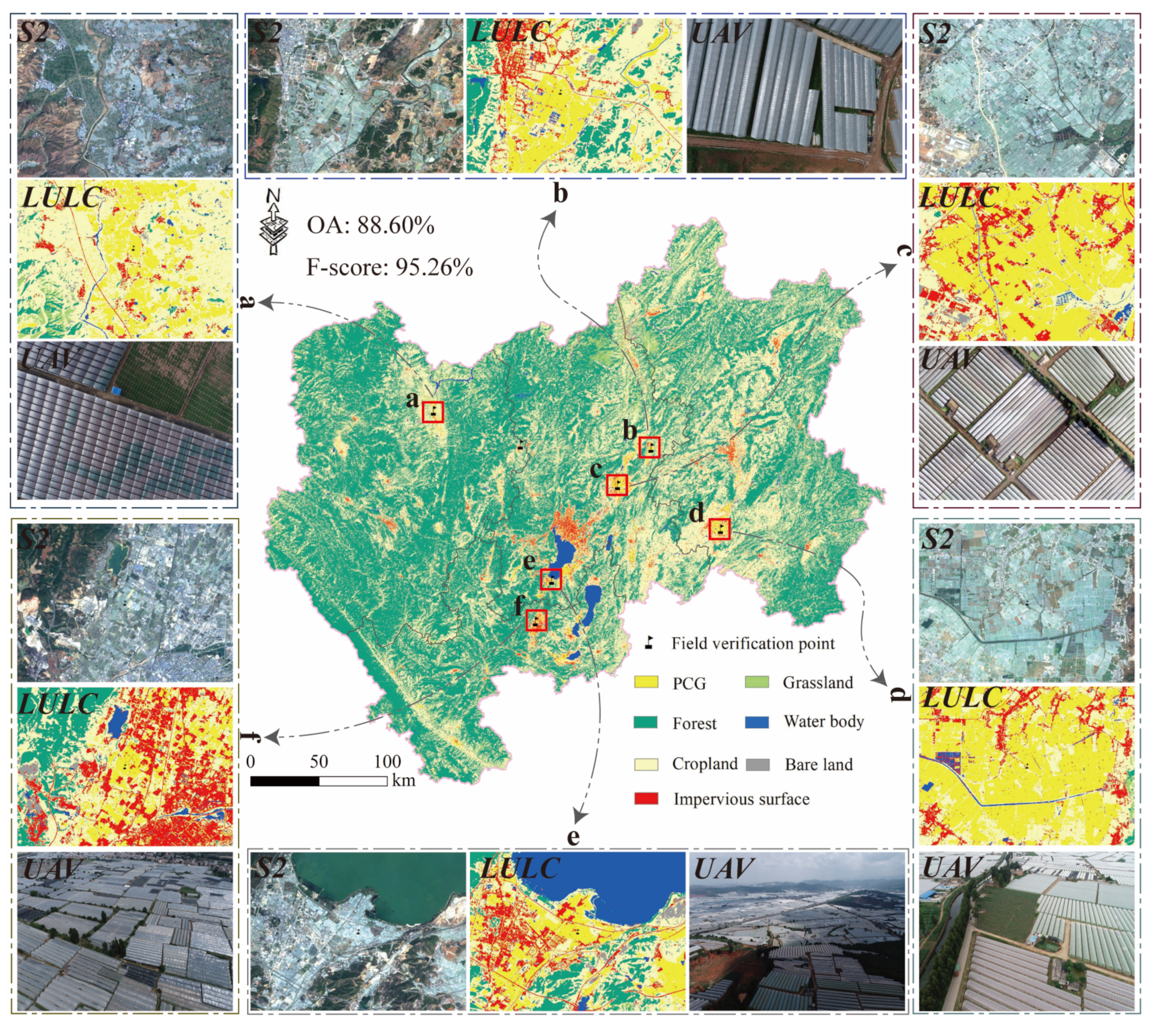
The study area is the CYP region, in the center of Yunnan Province, located in 23°19′~27°03′N, 100°43′~100°50′E (Figure 1), and is an important area for economic development in southwest China. It covers a total area of 9.4558 × 10⁴ km², with 4 autonomous prefectures/prefecture-level cities, including Kunming (the capital of Yunnan Province), Qujing, Yuxi, and Chuxiong [43]. CYP has large elevation differences, with many basins and intermountain dams. The region has a subtropical monsoon climate, with obvious dry and wet seasons [43]. In September 2015, given the context of China’s “Belt and Road” Initiative, the Central Yunnan New Area, China’s 15th national level new area, was designated in the CYP, which is planned to be developed into an important fulcrum of the southwest region facing south and southeast Asia. The abovementioned unique geographical advantages, policy support, and rich natural resources undoubtedly make the CYP a main grain-producing area and economic center in southwest China. According to the 2018 Statistical Yearbook, 38% of the population and 55% of the GDP in Yunnan Province are gathered in this region [44]. The vigorous economic development has promoted the transition from traditional agriculture to modern agriculture. Currently, it has formed a primary industry dominated by plateau flowers and modern agriculture. The development of these industries depends on a stable natural environment. However, the temperatures and precipitation in the dry and rainy seasons fluctuate strongly in CYP, especially with the emergence of extreme climate events in recent years, such as the once-in-a-century drought in 2009 and the heavy rainfall in 2010, which seriously threaten food security [43]. PCGs have the function of constant temperature and humidity, which can provide good growth environments for flowers, crops, etc., thereby increasing the yield [1]; thus, they are widely used in modern agriculture. In recent years, the PCGs of CYP have formed a large-scale “sea of PCGs” driven by economic development (Figure 1c,d).

2.2. Data Sources and Processing

The multiple datasets used in the current study mainly include remote sensing satellite images (i.e., S1, S2) and topographic data; these datasets have undergone geometric calibration and rectification, and the spatial consistency is relatively high, which can meet the needs of this research. In addition, all data were resampled to 10 m using the nearest neighbor interpolation function, and were defined as a unified geographic coordinate system (i.e., WGS_1984). We also collected auxiliary classification data, such as field-collected land use/land cover (LULC) samples and existing LULC products (i.e., GLOBELAND30 and ESA WorldCover). The main data are as follows.

2.2.1. Sentinel-1 SAR Image

The S1 SAR is derived from the Copernicus Programme of the ESA and equipped with a C-band (5.405 GHz) synthetic aperture radar sensor, which can provide SAR data in multiple strip scan modes (i.e., interferometric wide-swath (IW), wave, extra wide-swath, and strip map), multi-polarization modes (i.e., VV, HH, VV + VH, HH + HV), and dual-track modes (i.e., ascending, descending) (

Table 1. Sentinel-1 and 2 data parameters.

-	Sentinel-1 (A and B)	Sentinel-2 (A and B)
Mode/Format	GRD_IW	Level-1C
Frequency/Wavelength	5.405 GHz/5.5 cm	–
Orbital Mode	Ascending/Descending	–
Temporal Resolution (d)	6	5
Spatial Resolution (m)	10	10	20	60
Polarization/Band	VH	B2 (Blue)	B5 (Vegetation Red Edge-1)	B1 (Coastal aerosol)
	HH	B3 (Green)	B6 (Vegetation Red Edge-2)	B9 (Water vapor)
	VV + VH	B4 (Red)	B7 (Vegetation Red Edge-3)	B10 (Shortwave Infrared-Cirrus)
	HH + HV	B8 (NIR)	B8a (Vegetation Red Edge-4)	–
	–	–	B11 (Shortwave Infrared-1)	–
	–	–	B12 (Shortwave Infrared-2)	–

) [45]. The S1 SAR data in this study were obtained from the Ground Range Detected (GRD) product on GEE, with a maximum spatial resolution of 10 m, and have been preprocessed with the S-1 toolbox, including thermal noise removal, radiometric correction, and terrain correction (https://developers.google.com/earth-engine/datasets/catalog/COPERNICUS_S1_GRD (accessed on 7 September 2022)), so that the data quality is guaranteed. It can be directly accessed via the “COPERNICUS/S1_GRD” code. To minimize the influence of terrain, two polarization modes (i.e., VV, VH) in the IW strip mode were selected. Considering that high-quality SAR data need to completely cover the study area, and the time window covered by the PCG in CYP is the whole year, the time filter condition was set from January 1 to December 31 each year, and the spatial filter condition was the CYP region. Finally, the median of all pixels in all matched band stacks was calculated to synthesize the annual S1 SAR data.

2.2.2. Sentinel-2 Optical Image

The S2 two-satellite constellation (i.e., S2 A and B), also from ESA’s Copernicus Programme, carries a Multi Spectral Instrument (MSI) [46]. It can provide 13 spectral bands ranging from 443 to 2190 nm and a spatial resolution from 10 to 60 m, with a revisit time of 5 days (Table 1). S2 data in GEE includes Top-Of-Atmosphere (TOA) reflectance and Surface Reflectance (SR) data. In terms of data availability, SR data are available nearly two years later than TOA data. Considering that the longer monitoring period represents the greater application value, the S2-Level-1C product was initially selected for this study, and is the TOA data that has been ortho-corrected and sub-pixel-level geometric fine-correction [33]; it could be directly accessed in GEE through the “COPERNICUS/S2” code (https://developers.google.com/earth-engine/datasets/catalog/COPERNICUS_S2 (accessed on 7 September 2022)). In practice, it is extremely challenging to use a single scene image for LULC classification due to the cloudy nature of the plateau area. The dense time stack method can replace a co-located cloudy image with another image to create a sharp image [47]. Through multiple tests in the GEE programming environment, the time interval was set from January 1st to December 31st every year, and all S2 TOA data with cloud cover less than 12% were obtained by the dense time stack method, and the median reducer function was further used to synthesize it into high-quality annual composite images [40]. Then, original S2-TOA data were atmospherically corrected using the py6s module, since the calculation of spectral indices was involved later (https://github.com/samsammurphy/gee-atmcorr-S2/blob/master/jupyer_notebooks/sentinel2_atmospheric_correction.ipynb (accessed on 8 September 2022)) [48]. Finally, all bands were resampled to 10 m using the default nearest neighbor interpolation function.

2.2.3. Shuttle Radar Topography Mission (SRTM) Terrain Data

The SRTM data, provided by NASA, contains a global digital elevation model, with a spatial resolution of 30 m [49]. The SRTM V3 product was selected as auxiliary data to provide topographic features. Data processing was performed by programming in GEE: (1) the SRTM data were accessed by the “USGS/SRTMGL1_003” code (https://developers.google.com/earth-engine/datasets/catalog/USGS_SRTMGL1_003 (accessed on 10 September 2022)) and cropped according to the administrative boundary of CYP; (2) the nearest neighbor interpolation function was used to convert it to the same spatial resolution as the S2 data; (3) the “ee.Algorithms.Terrain()” function was used to calculate terrain features.

2.2.4. Reference Data for Supervised Classification

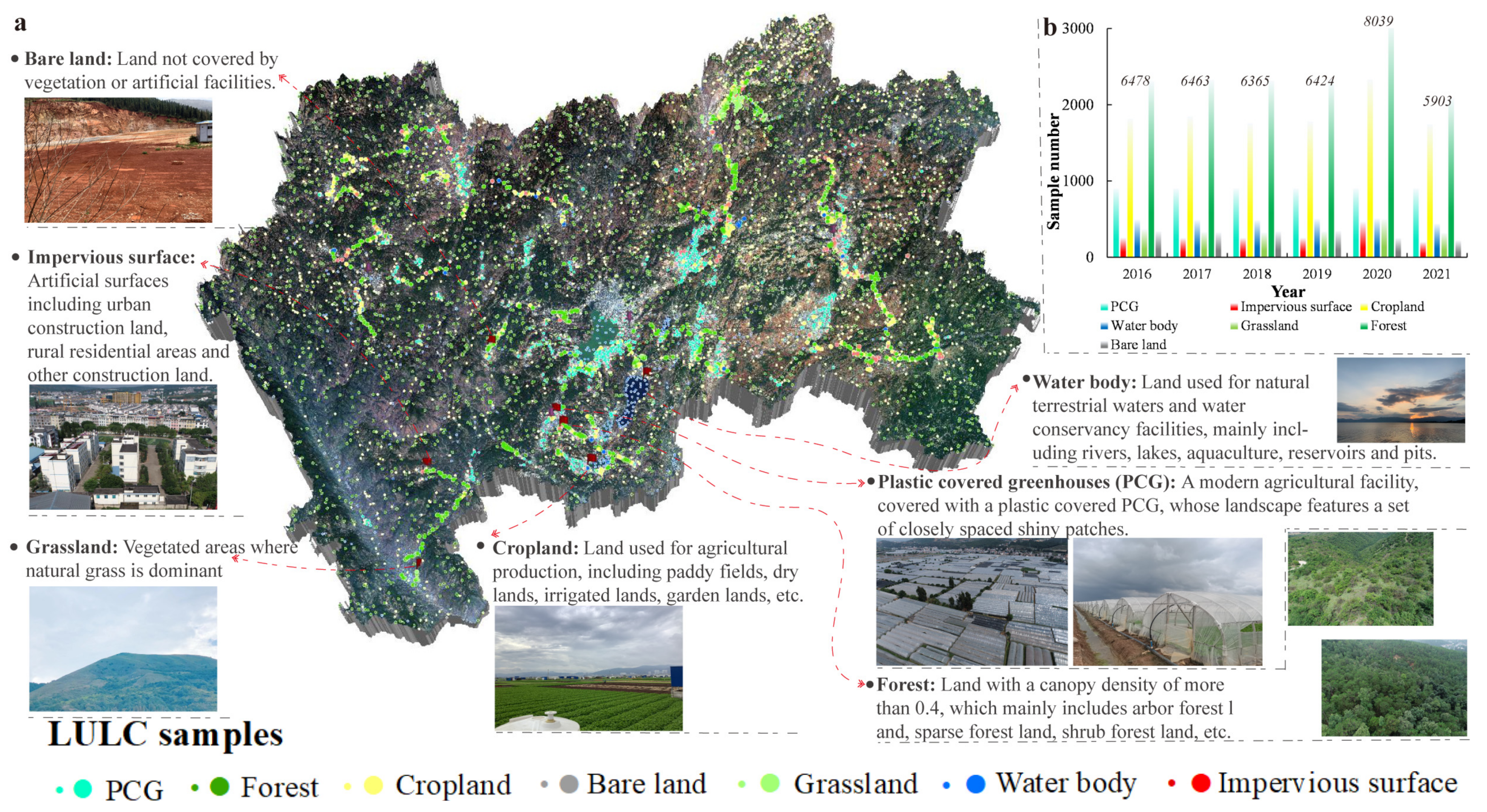
The effective identification of PCGs by supervised machine learning methods in GEE relies on reliable and accurate LULC samples [1]. To obtain high-quality samples, we conducted detailed land surveys in CYP in 2020 and 2021 and achieved many remarkable gains. As shown in Figure 2a, first, according to the survey results and previous research [50], we determined that the classification system includes the following seven main LULC types: PCG, cropland, forest, grassland, water body, impervious surface, and bare land; in addition, we collected a large number of field LULC samples with handheld GPS units and took photos for evidence. Considering that samples in the supervised classification need to be evenly distributed, but the field samples were lacking in remote areas, we screened and expanded field-collected LULC samples based on 2020 high-resolution Google images and the 2020 GLOBELAND30 product (http://globallandcover.com/) to form a sample database. With this sample library as a reference, we collected annual LULC samples from 2016 to 2021 through visual interpretation on Google historical images and S2 true color images from the same period (Figure 2b), with a total number of 39,672 samples. Ultimately, the random number algorithm of the GEE platform was used to divide various samples into training samples (70%) and validation samples (30%), which were used for classification algorithm training and subsequent accuracy verification, respectively.

2.3. Methods

2.3.1. Overview of the Methodology

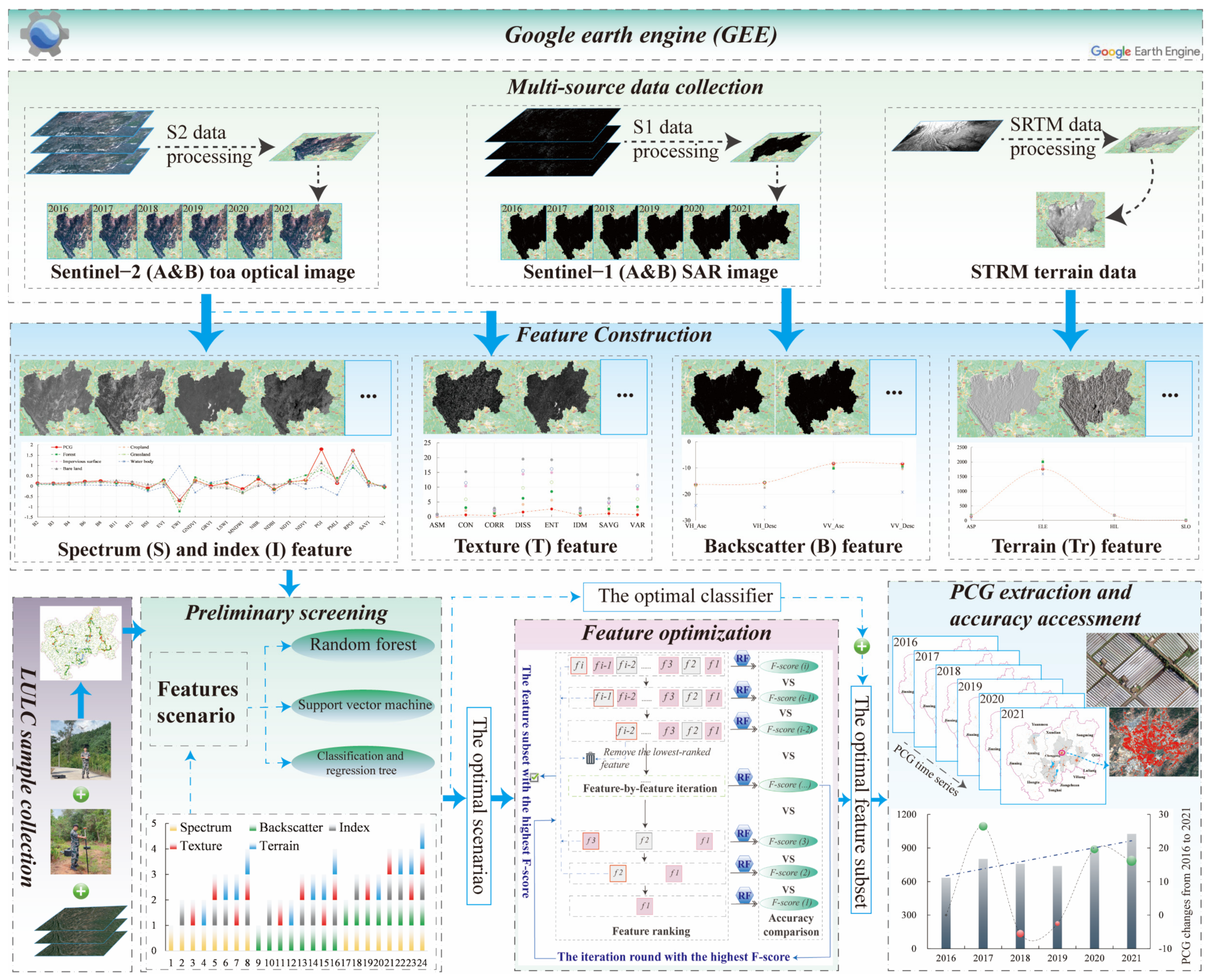
The proposed research framework was mainly implemented by programming on the GEE platform. Specifically, we: (i) collected multi-source data (i.e., S1 SAR, S2, and SRTM data) directly on the GEE platform and preprocessed it, and then constructed multi-feature scenarios covering spectrum, backscatter, index, texture, and terrain features based on these data; (ii) selected three well-received LULC machine learning classifiers (i.e., CART, RF, and SVM) to construct classification algorithms based on a large number of reliable LULC samples and different feature scenarios, and evaluated the accuracy of each classifier in different feature scenarios each year to avoid the absolute impact of a single classifier or a single scenario, so as to initially screen the best classifier and original feature scenario; (iii) assessed the feature importance of the original feature set each year through the RF model, and eliminated the feature with the lowest importance, and the remaining features continued to participate in the classification; in this way, we selected the best feature subset of different years through multiple iterations; (iv) compiled a classification algorithm based on the best classifier and the best feature subset, extracted the PCGs in CYP from 2016 to 2021, and performed accuracy and vision evaluations; (v) mapped the PCG dynamic spectrum and analyzed its spatiotemporal features. The workflow is illustrated in Figure 3.

2.3.2. Feature Construction

The selection of feature variables is crucial for remote sensing classification, and previous studies have pointed out that the combination of multiple features can effectively improve the classification accuracy [1]. As artificial facilities, PCGs are mixed, complex, and heterogeneous due to the differences in material types, crop structures, and satellite sensors [20]. Visually, the spectral characteristics of PCGs are very similar to those of bare land and impervious surfaces, which are difficult to distinguish. Especially in areas with complex LULC types, the remote sensing extraction of PCGs is affected by many factors. Thus, in order to reduce the mapping error, the present study deeply considered the attributes of PCGs and their spatial characteristics in CYP, and tested some new features while referring to the results of previous studies (e.g., Aguilar et al. [39]; Ou et al. [20]). Ultimately, five types of features, including spectrum, backscatter, index, texture, and terrain, were constructed, with a total of 39 feature factors.

(1)

Spectrum (S) and index (I) features

The spectrum and its derived remote sensing indices are the most widely used features in LULC classification. For the former, considering the band redundancy and referring to previous studies [6], only bands at 10 m (B2-Blue, B3 -Green, B4-Red, and B8-NIR) and 20 m (B6-Red edge, B11-shortwave infrared-1, and B12-shortwave infrared-2) resolutions were selected (Table 2). For the latter, the previous research has revealed that remote sensing indices can effectively enhance the spectral characteristics of specific objects [1]. For example, the normalized difference vegetation index (NDVI) can effectively extract vegetation; similarly, the modified normalized difference water index (MNDWI) and the normalized difference built-up index (NDBI) can effectively identify water bodies and impervious surfaces, respectively. Sixteen commonly used remote sensing indices were calculated on the GEE platform using original spectral bands of S2 (Table 2). Among them, the normalized difference tillage index (NDTI, [51]) and retrogressive plastic greenhouse index (RPGI, [9]) were mainly used to identify PCGs.

(2)

Texture (T) features

The texture feature is an important window that can reflect the remote sensing image information excluding the spectrum feature, and the texture characteristics of PCGs can make up for spectral limitations due to their special structure. Considering the PCGs’ characteristics, and referring to previous studies [20,52], the eight most commonly used texture indicators were selected to participate in the feature space (Table 2), including the angular second moment, contrast, correlation, variance, inverse difference moment, sum average, entropy and dissimilarity. The “ee.glcmTexture(size, kernel, average)” function provided by GEE can quickly calculate the above texture features based on the gray level co-occurrence matrix (GLCM). The GLCM algorithm requires a grey-level 8-bit image as input [52], which is generally calculated based on a certain reference band of S2 images, but there is no unified standard for the band (e.g., Chen et al. [53]: B12; Lin et al. [1]: B2; Ou et al. [20]: B8). In the current study, referring to the formula (i.e., $\mathrm{Gray}=(0.3\times \mathrm{NIR})+(0.59\times \mathrm{RED})+(0.11\times \mathrm{GREEN})$) proposed by Tassi and Vizzari [52], texture features were constructed based on a grey image that was calculated by a linear combination of the NIR, red, and green bands of the initial S2 composite image.

(3)

Backscatter (B) feature

As an active imaging radar, SAR can make up for the optical data defects that are easily affected by observation conditions. The high dielectric properties, special geometry and radar echo characteristics of PCGs give them a strong backscattered signal, and the addition of SAR will help to improve the PCG extraction accuracy. S1 SAR has a dual-orbit multi-polarization function, and both VH and VV polarization information can contain vegetation-ground interactions [33]. Considering that previous studies have pointed out that dual-orbit data can weaken the shadow and overlay of SAR images in mountainous areas, dual-polarization data are beneficial for improving the accuracy of ground object recognition [54]. Therefore, the feature construction strategy was to cross-integrate all the dual-orbital and dual-polarization multi-temporal SAR data in the IW mode of the study area throughout the year through the dense time stack method, and synthesize the interannual S1 SAR data with the mean value, which includes four backscatter feature bands, namely, “VV_Asc”, “VH_Asc”, “VV_Desc”, and “VH_Desc” (Table 2).

(4)

Terrain (Tr) feature

The spatial distribution of PCGs is greatly affected by the complex terrain in CYP, which is usually distributed in the relatively flat intermountain dam region, whereas rarely in high-altitude or high-slope mountainous regions. Thus, terrain features should be incorporated into the feature variables. Based on the SRTMGL1_003 data provided by the GEE platform, this study calculated four terrain features using the “ee.Algorithms. Terrain (input)” function, including elevation, slope, aspect, and hillshade (Table 2).

Table 2. All the selected feature factors in this study.

Feature Types	Feature Factors	Calculation Methods	References
Spectrum Features (S)	B2 (Blue, B)	Extracting specific band from the S2 annual composite images	Nemmaoui et al. [21]
	B3 (Green, G)
	B4 (Red, R)
	B6 (Vegetation Red Edge-2)
	B8 (Near infrared, NIR)
	B11 (Shortwave Infrared-1, SWIR1)
	B12 (Shortwave Infrared-2, SWIR2)
Index Features (I)	BSI (Bare Soil Index)	((SWIR1 + R) − (NIR + B))/((SWIR1 + R) + (NIR + B))	Roy et al. [55]
	VI (Vegetation indices)	((SWIR1 − NIR)/(SWIR1 + NIR))*((NIR − R)/(NIR + R))	He et al. [56]
	EVI (Enhanced Vegetation Index)	2.5*(NIR − R)/(NIR + 6*R − 7.5*B + 1)	Jiang et al. [57]
	EWI (Enhanced Water Index)	(G − SWIR1)/(G + SWIR1)) + (G − NIR)/(G + NIR) − (NIR − R)/(NIR + R)	Wang et al. [58]
	NDVI (Normalized Difference Vegetation Index)	(NIR − R)/(NIR + R)	Rouse et al. [59]
	GNDVI (Green NDVI)	(NIR − G)/(NIR + G)	Phadikar and Goswami [60]
	GRVI (Green Red Vegetation Indices)	(G − R)/(G + R)	Khadanga and Jain [61]
	LSWI (Land Surface Water Index)	(NIR − SWIR1)/(NIR + SWIR1)	Chandrasekar et al. [62]
	MNDWI (Modified Normalized Difference Water Index)	(G − SWIR1)/(G + SWIR1)	Xu [63]
	NBR (Normalized Burn Ratio)	(NIR − SWIR2)/(NIR + SWIR2)	Picotte et al. [64]
	NDBI (Normalized Difference Built-up Index)	(SWIR1 − NIR)/(SWIR1 + NIR)	Aziz [65]
	NDTI (Normalized Difference Tillage Index)	(SWIR1 − SWIR2)/(SWIR1 + SWIR2)	Fernández-Buces et al. [51]
	SAVI (Soil Adjusted Vegetation Index)	(1.5*(NIR − R))/(NIR + R + 0.5)	HUETE [66]
	PGI (Plastic Greenhouse Index)	(100*R*(NIR − R))/(1− (NIR + B + G)/3)	Yang et al. [9]
	PMLI (Plastic-Mulched Landcover Index)	(SWIR1 − R)/(SWIR1 + R)	Lu et al. [25]
	RPGI (Retrogressive Plastic Greenhouse Index)	(100*B)/(1 − (NIR + B + G)/3)	Yang et al. [9]
Texture Features (T)	ASM (Angular Second Moment)	The grey-level 8-bit image calculated by the (0.3*NIR)+(0.59*R)+(0.11*G) formula was used as an input variable to input the ee. glcmTexture(size, kernel, average) function provided by the GEE platform to construct texture features.	Tassi and Vizzari [52]
	CON (Contrast)
	CORR (Correlation)
	DISS (Dissimilarity)
	ENT (Entropy)
	IDM (Inverse Difference Moment)
	SAVG (Sum Average)
	VAR (Variance)
Backscatter Features (B)	VH_Asc	Median value of all bands of VH cross polarization in ascending (Asc) orbit	This study
	VH_Desc	Median value of all bands of VH cross polarization in descending (Desc) orbit
	VV_Asc	Median value of all bands of VV monopolarization in ascending (Asc)/descending (Desc) orbit
	VV_Desc
Terrain Features (Tr)	ASP (Aspect)	Based on the SRTMGL1_003 terrain data, the selected terrain features were calculated using ee.Algorithms.Terrain (input) function provided by the GEE platform.	Lin et al. [1]
	ELE (Elevation)
	HIL (Hillshade)
	SLO (Slope)

R, G, B, NIR, SWIR1, and SWIR2 in the formula represent B4 (Red), B3 (Green), B2 (Blue), B8 (NIR), B11 (SWIR1), and B12 (SWIR2) in the original spectral band of S2 data, respectively.

Table 2. All the selected feature factors in this study.

Feature Types	Feature Factors	Calculation Methods	References
Spectrum Features (S)	B2 (Blue, B)	Extracting specific band from the S2 annual composite images	Nemmaoui et al. [21]
	B3 (Green, G)
	B4 (Red, R)
	B6 (Vegetation Red Edge-2)
	B8 (Near infrared, NIR)
	B11 (Shortwave Infrared-1, SWIR1)
	B12 (Shortwave Infrared-2, SWIR2)
Index Features (I)	BSI (Bare Soil Index)	((SWIR1 + R) − (NIR + B))/((SWIR1 + R) + (NIR + B))	Roy et al. [55]
	VI (Vegetation indices)	((SWIR1 − NIR)/(SWIR1 + NIR))*((NIR − R)/(NIR + R))	He et al. [56]
	EVI (Enhanced Vegetation Index)	2.5*(NIR − R)/(NIR + 6*R − 7.5*B + 1)	Jiang et al. [57]
	EWI (Enhanced Water Index)	(G − SWIR1)/(G + SWIR1)) + (G − NIR)/(G + NIR) − (NIR − R)/(NIR + R)	Wang et al. [58]
	NDVI (Normalized Difference Vegetation Index)	(NIR − R)/(NIR + R)	Rouse et al. [59]
	GNDVI (Green NDVI)	(NIR − G)/(NIR + G)	Phadikar and Goswami [60]
	GRVI (Green Red Vegetation Indices)	(G − R)/(G + R)	Khadanga and Jain [61]
	LSWI (Land Surface Water Index)	(NIR − SWIR1)/(NIR + SWIR1)	Chandrasekar et al. [62]
	MNDWI (Modified Normalized Difference Water Index)	(G − SWIR1)/(G + SWIR1)	Xu [63]
	NBR (Normalized Burn Ratio)	(NIR − SWIR2)/(NIR + SWIR2)	Picotte et al. [64]
	NDBI (Normalized Difference Built-up Index)	(SWIR1 − NIR)/(SWIR1 + NIR)	Aziz [65]
	NDTI (Normalized Difference Tillage Index)	(SWIR1 − SWIR2)/(SWIR1 + SWIR2)	Fernández-Buces et al. [51]
	SAVI (Soil Adjusted Vegetation Index)	(1.5*(NIR − R))/(NIR + R + 0.5)	HUETE [66]
	PGI (Plastic Greenhouse Index)	(100*R*(NIR − R))/(1− (NIR + B + G)/3)	Yang et al. [9]
	PMLI (Plastic-Mulched Landcover Index)	(SWIR1 − R)/(SWIR1 + R)	Lu et al. [25]
	RPGI (Retrogressive Plastic Greenhouse Index)	(100*B)/(1 − (NIR + B + G)/3)	Yang et al. [9]
Texture Features (T)	ASM (Angular Second Moment)	The grey-level 8-bit image calculated by the (0.3*NIR)+(0.59*R)+(0.11*G) formula was used as an input variable to input the ee. glcmTexture(size, kernel, average) function provided by the GEE platform to construct texture features.	Tassi and Vizzari [52]
	CON (Contrast)
	CORR (Correlation)
	DISS (Dissimilarity)
	ENT (Entropy)
	IDM (Inverse Difference Moment)
	SAVG (Sum Average)
	VAR (Variance)
Backscatter Features (B)	VH_Asc	Median value of all bands of VH cross polarization in ascending (Asc) orbit	This study
	VH_Desc	Median value of all bands of VH cross polarization in descending (Desc) orbit
	VV_Asc	Median value of all bands of VV monopolarization in ascending (Asc)/descending (Desc) orbit
	VV_Desc
Terrain Features (Tr)	ASP (Aspect)	Based on the SRTMGL1_003 terrain data, the selected terrain features were calculated using ee.Algorithms.Terrain (input) function provided by the GEE platform.	Lin et al. [1]
	ELE (Elevation)
	HIL (Hillshade)
	SLO (Slope)

R, G, B, NIR, SWIR1, and SWIR2 in the formula represent B4 (Red), B3 (Green), B2 (Blue), B8 (NIR), B11 (SWIR1), and B12 (SWIR2) in the original spectral band of S2 data, respectively.

2.3.3. Machine Learning-Based Supervised Classifier

Previous studies have reported that the machine learning algorithm is superior to other supervised classifiers [27]. In the current study, three machine learning classifiers on the GEE platform that were recognized for their good performance, namely, CART, SVM, and RF [33], were selected to identify the optimal classifier for PCG identification in the CYP region.

(1)

CART classifier

The CART algorithm was proposed by Breiman et al. [67]. Its basic principle is a tree-growing process through the cyclic binary recursive partitioning of test variables (feature vectors) and target variables (actual feature types). The process stops when the data space cannot be split any further, and finally the decision tree model is obtained by fitting each dichotomy rule. It is worth noting that a larger depth can result in a complex decision tree with a possibly higher accuracy but also raises the risks of overfitting.

In the tree-growing procedure, the Gini index of economics is used as the criterion for selecting the best test variable and segmentation threshold. The formula for the Gini index is as follows:

$$\mathrm{GI}=1-{\displaystyle \sum _{m=1}^M{p}^2(\frac{m}{x})}$$

(1)

$$p(\frac{m}{x})=\frac{n_m(x)}{n(x)};\hspace{1em}{\displaystyle \sum _{m=1}^M{p}^2(\frac{m}{x})}=1$$

(2)

where GI represents the Gini index, $m$ is the number of classes, $p(\frac{m}{x})$ is the probability value, indicating the possibility of belonging to the $m\mathrm{th}$ category when the test variable value of a sample randomly selected from the training sample is $x$, $n(x)$ is the number of samples in the training sample when the test variable value is $x$, and $n(x)$ is the number of samples belonging to category $m\mathrm{th}$ when the test variable value is $x$.

(2)

RF classifier

Breiman et al. [68] first proposed the RF algorithm, which is an integrated learning technique based on CART sets. A detailed review of the RF classifier algorithm is beyond the scope of this paper, and more information can be found in previous articles. The principles of the RF classifier are as follows: ① The bootstrap sampling strategy is used to randomly sample from the original sample set to create training samples; ② multiple decision trees are built and integrated based on training samples, and each decision tree outputs a rule to form a forest; and ③ the final classification results are generated according to the voting method, and the remaining samples are used for internal cross testing to evaluate the classification accuracy. RF is widely used for remote sensing classification due to its high robustness, strong data compatibility, and good performance advantages [20]. Similar to the CART algorithm, the Gini index is often used in the RF classifier as a measurement for the best segmentation selection which maximizes dissimilarity between classes (Equations (1) and (2)). Two parameters need to be set to use the RF algorithm in GEE: ① ntree represents the number of decision trees, and this study determines that the optimal ntree was 500 after many experiments; ② mty, which represents the square root of the number of features, was set as the default value.

(3)

SVM classifier

SVM is a nonparametric machine learning algorithm which was proposed by CORTES and VAPNIK [69]. Its core idea is to find the optimal hyperplane in a high-dimensional space as a decision function. Specifically, ① the nonlinearly separable data can be mapped to a high-dimensional space through the SVM algorithm to realize linear separability; ② in the sample feature space, the optimal separation hyperplane is found through the guidance of the kernel function to maximize the distance between different classes, and, finally, the input vector is classified into different categories. The SVM classifier has a high generalization ability and low sample quality requirements and has been widely used in the automatic classification of remote sensing images.

2.3.4. Feature Optimization Strategy

For machine learning classifiers, the promotion effect of the feature dimension on the classification accuracy is not absolute. In other words, more feature dimensions may not lead to a higher classification accuracy. In fact, too many features may also decrease the learning ability of the classifier, which is known as the “dimension disaster” [37]. A total of 39 feature factors were constructed in the present study, including seven spectrum features, four backscatter features, sixteen index features, eight texture features, and four terrain features. To avoid the abovementioned “dimension disaster”, redundant features were deleted through feature optimization to reduce the feature dimensions, thereby improving the classification accuracy and performance. Recursive feature elimination (RFE) was first proposed by Guyon et al. [70] in the context of SVM. In recent years, many scholars have performed RFE algorithm in the RF model (i.e., RF-RFE), and it was effectively applied to feature optimization for different classification tasks (e.g., Darst et al. [71]; Grabska et al. [72]; Gregorutti et al. [73]). We applied this feature optimization strategy to extract PCG for the first time. The interpretation of the RF-RFE principle is as follows (Figure 4): (1) The RF classification model is fitted based on the original feature scene of the initial screening, all features are ranked according to their importance, and the lowest-ranked feature is removed; (2) the remaining features continued to participate in the next round of classification and importance ranking, the lowest-ranked feature will be deleted again, and so on, and all the feature factors were iterated; (3) the iteration round with the highest accuracy and the corresponding feature factors was selected, and the latter was the best feature subset.

2.3.5. Accuracy Assessment

In the present study, the classifier comparison, preliminary screening of original feature scenarios, and feature optimization require a quantification of accuracy to select the best classifiers and features. The confusion matrix is a standard method for the accuracy evaluation, which includes four parameters, namely, the overall accuracy (OA), producer’s accuracy (PA), user’s accuracy (UA), and Kappa coefficient [1]. We constructed a confusion matrix based on randomly selected validation samples (30% of the total samples) and chose two complementary indicators to evaluate the classification accuracy. The first was OA, which evaluated the effectiveness of the overall algorithm; the second was the F-score, also known as the across-site robustness, which measured the identification accuracy of PCG by balancing the relationship between PA and UA [14,39]. The above metrics were calculated by the following formulas:

$$\mathrm{OA}=\frac{{\mathrm{TP}}_{\mathrm{all}}}{{\mathrm{P}}_{\mathrm{all}}}\times 100\%$$

(3)

$${\mathrm{UA}}_{\mathrm{PCG}}=\frac{{\mathrm{TP}}_{\mathrm{PCG}}}{{\mathrm{P}}_{\mathrm{PCG}}}\times 100\%$$

(4)

$${\mathrm{PA}}_{\mathrm{PCG}}=\frac{{\mathrm{TP}}_{\mathrm{PCG}}}{{\mathrm{C}}_{\mathrm{PCG}}}\times 100\%$$

(5)

$$\mathrm{F}-\mathrm{score}=\frac{({\beta }^2+1)\times {\mathrm{UA}}_{\mathrm{PCG}}\times {\mathrm{PA}}_{\mathrm{PCG}}}{{\beta }^2\times {\mathrm{PA}}_{\mathrm{PCG}}+{\mathrm{UA}}_{\mathrm{PCG}}}\times 100\%$$

(6)

where ${\mathrm{TP}}_{\mathrm{all}}$ is the number of all LULC samples that are correctly classified; ${\mathrm{P}}_{\mathrm{all}}$ is the sum of LULC samples used for validation; ${\mathrm{TP}}_{\mathrm{PCG}}$ represents the total number of pixels that are correctly classified as PCGs; ${\mathrm{P}}_{\mathrm{PCG}}$ represents the total number of pixels of PCGs; ${\mathrm{C}}_{\mathrm{PCG}}$ represents the total number of pixels of PCGs in the validation sample; and $\beta$ represents the weight relationship between ${\mathrm{UA}}_{\mathrm{PCG}}$ and ${\mathrm{PA}}_{\mathrm{PCG}}$, which is set to 1 according to previous research by Xiong et al. [13].

3. Results

3.1. Preliminary Screening of Feature Scenarios and Classifiers

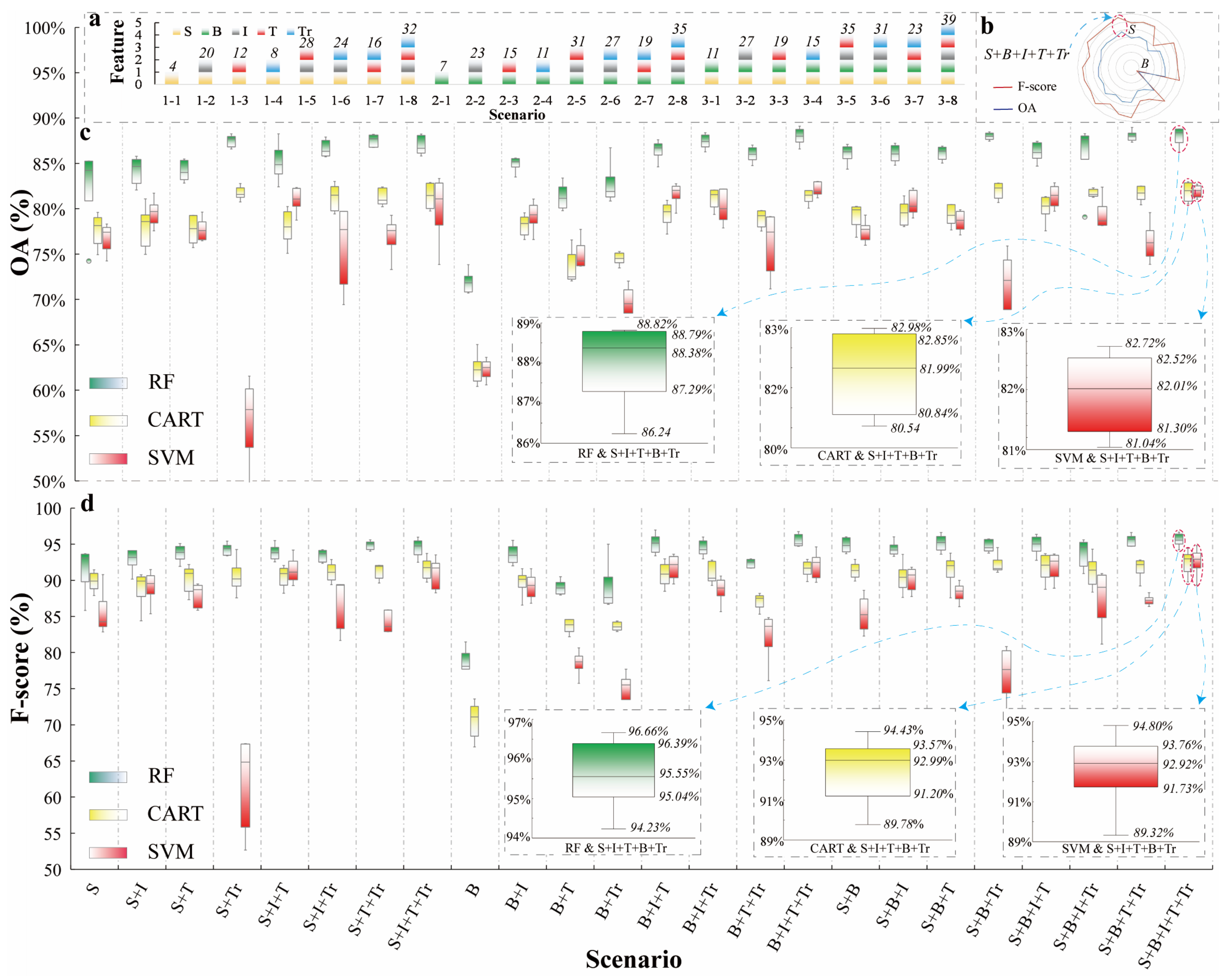
To preliminarily screen the best classifier and feature scenario for PCG identification, the classification accuracy produced by the combination of different feature scenes and classifiers was evaluated each year. First, five types of features were combined into different scenarios. Considering the difference between active/passive remote sensing data features in PCG extraction was one of the aims of this study. Thus, the backscatter (B) features of S1 SAR and the spectrum features (S) of S2 were superimposed with other features (i.e., index (I), texture (T), and terrain (Tr) feature) to form scenarios numbered 1-1 to 1-8 and 2-1 to 2-8, respectively; then, the feature combination of S1 SAR and S2 was superimposed with other features to form scenarios numbered 3-1 to 3-8 (Figure 5a). Scenario 3-8 was S + B + I + T + Tr, covering 5 types of features and a total of 39 feature factors. Based on different scenarios, the RF, SVM, and CART classifiers were used to extract the LULC of CYP each year and evaluate the accuracy.

The 6-year average accuracy of different scenarios demonstrates (Figure 5b) that among the scenarios that were constructed based on S, the F-score and OA of the S + I + T + Tr scenario were the highest at 92.39% and 82.88%, respectively, while those of the S scenario were the lowest at 88.96% and 79.10%, respectively. In the scenarios constructed based on B, the F-score and OA of the B + I + T + Tr scenario were the highest (93.05% and 83.82%), while those of the B scenario were the lowest among all the scenarios, at 64.09% and 65.59%, respectively. In the scenarios constructed based on S + B, the scenarios with the lowest F-score and OA were S + B (90.52%) and S + B + Tr, respectively (80.35%), while the S + B + I + T + Tr scenario had the highest F-score and OA values among all the scenarios at 93.59% and 83.95%, respectively. This result indicated that more features will lead to a higher accuracy.

The accuracy of the combination of 3 classifiers and 24 scenarios was comprehensively evaluated (Figure 5c,d). The statistics demonstrated that the combination of the RF classifier and the S + I + T + B + Tr scenario created the highest F-score and OA, at 95.60% and 88.04%, respectively; and CART and SVM also achieved the highest accuracy in the S + I + T + B + Tr scenario, the difference between the F-score and OA of the two was only −0.13% (92.52% vs. 92.65%) and −0.06% (81.87% vs. 81.94%). Focusing on a classifier, although the accuracy fluctuated among different scenarios, three classifiers demonstrated an upwards trend in the F-score and OA with an increase in features. For the RF classifier, the F-score and OA of the S + I + T + B + Tr scenario were 0.74 and 1.92% higher, respectively, than those of the S + B scenario, and they were higher than those of the S and B scenario. The same regularity also appeared in the SVM and CART classifiers. This further proved that an increase in features could generally improve the classification accuracy even in different classifiers. Focusing on different classifiers, the F-score and OA of the RF classifier were higher than those of CART and SVM in all scenarios. The 6-year average accuracy of the three classifiers illustrated that the RF classifier had the highest accuracy, with an F-score and OA of 93.16% and 85.35%, respectively. This was followed by CART, with an F-score and OA of 89.39% and 78.83%, respectively. SVM had the lowest accuracy, with an F-score and OA of 83.90% and 76.63%, respectively, which indicated that the RF classifier was more suitable for extracting PCGs. In general, the combination of the S + I + T + B + Tr scenarios and RF classifiers demonstrated significant advantages for both overall LULC classification and PCG extraction; consequently, in preliminary screening, they were used as the best feature scenario and classifier, respectively.

3.2. Feature Optimization Based on RF-RFE Method

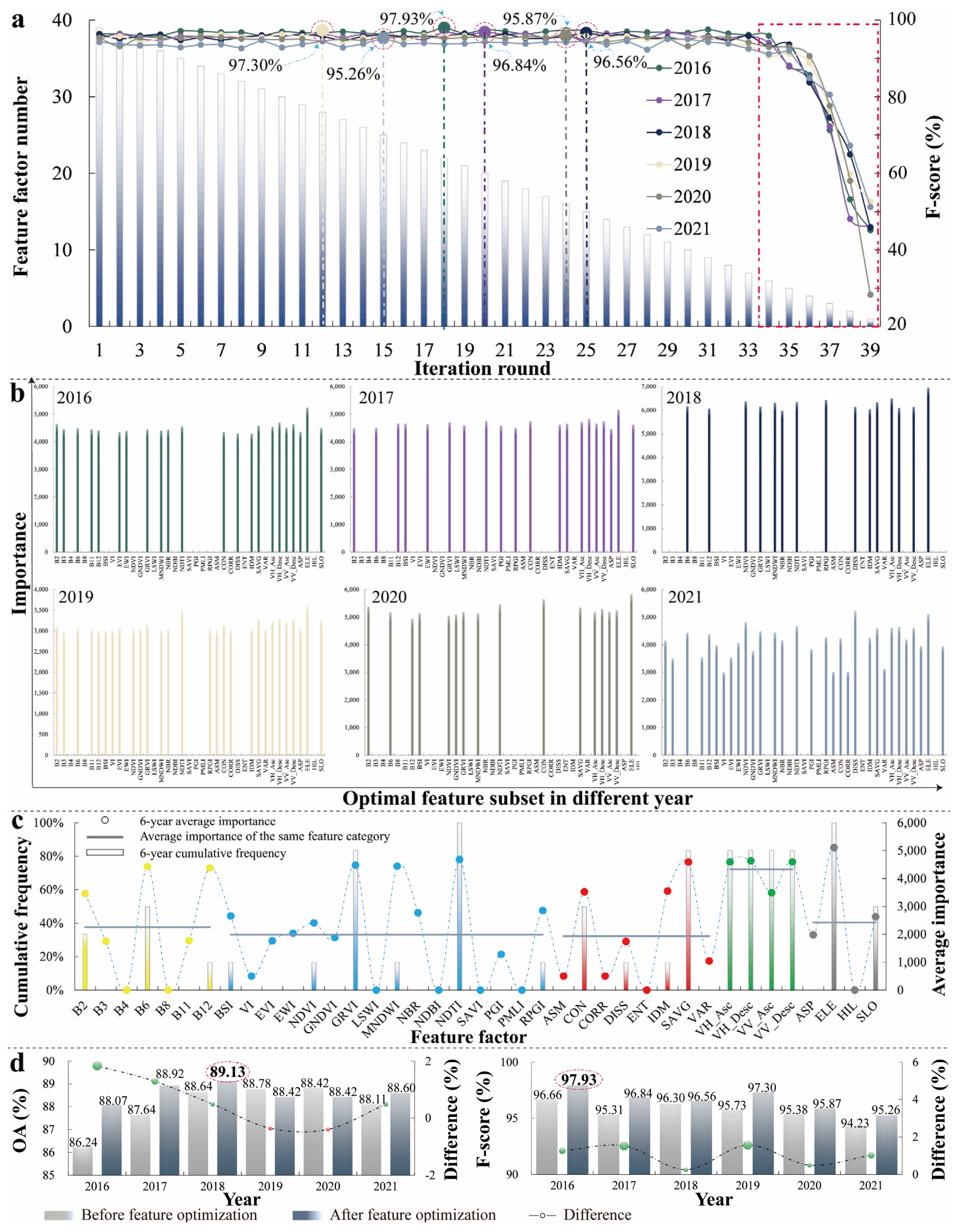
The feature importance was evaluated by the RF model, and the higher the importance, the greater the contribution to the classification results [47]. Based on the importance order of the feature factors in each round, 39 rounds of the iteration were performed for the 39 feature factors of the S + B + I + T + Tr scenario (Figure 6a), and the F-score of each round was evaluated to select the feature subset corresponding to the round with the highest F-score. The statistics demonstrated that the F-score reached the highest value (97.93%) when it was iterated to 18 rounds (22 features) in 2016. The F-score reached the highest value when it was iterated to the 20th (96.84%), 25th (96.56%), 12th (97.30%), 24th (95.88%), and 15th (95.26%) rounds in 2017, 2018, 2019, 2020, and 2021, respectively. Another finding was that the F-score curve of all years fluctuated slightly before an iteration to 34 rounds (6 features) and then dropped sharply with a decrease in features, which indicated that too few features would be extremely unfavorable for recognizing PCGs.

Figure 6b plots the best feature subset corresponding to the iteration rounds with the highest F-score in different years, which revealed that the best feature subsets were different in different years. Further statistics demonstrated (Figure 6c) that the top five feature factors were ranked by the 6-year average importance in descending order, as: ELE (5104.91) > NDTI (4685.23) > VH_Desc (4637.22) > VH_Asc (4595.91) > SAVG (4592.33). Coincidentally, the top five most frequent feature factors among the top ten features of the best feature subset over the past 6 years were also ranked as follows: ELE (100%) = NDTI (100%) > VH_Desc (83.33%) = VH_Asc (83.33%) = SAVG (83.33%). For the feature category, the average importance of the backscatter feature was the highest (4329.45), followed by the terrain feature (2427.65), spectrum feature (2255.98), index feature (1985.21), and texture features (1930.70). For intra-category feature factors, the factors with the highest contributions in each feature category were VH_Desc (4637.22), ELE (5104.91), B6 (4431.27), NDTI (4685.23), and SAVG (4592.04), respectively.

Figure 6d compares the classification accuracy of the optimal feature subset after feature optimization with the optimal accuracy before optimization in the same year. The OA was higher than that before feature optimization except for a slight decrease in 2019 and 2020, while the F-score surpassed in all years. Additional statistics demonstrated that the average F-score and OA after feature optimization were 0.56% (88.60% vs. 88.04%) and 1.03% (96.63% vs. 95.60%) higher than those before optimization, respectively, indicating that feature optimization had a positive effect on the overall LULC classification and PCG recognition.

3.3. Accuracy Assessment

The PCG mapping result of the highest F-score was obtained by combining the RF classifier and the optimal feature subset of different years. Quantitative evaluation of classification accuracy (Figure 6d: OA/F-score after feature optimization) demonstrated that the highest OA was 89.13% in 2018, which was also more than 88% in other years. The average F-score of PCG exceeded 95.00%, and the highest value appeared in 2016 (97.93%). The results of PCG mapping in 2021 were visually inspected by comparing the classification results of six typical regions where PCGs were concentrated in CYP with satellite images and UAV aerial photos (Figure 7). The PCGs and other LULC landscapes extracted in this study were found to have good spatial consistency with satellite images at the macro scale; even in complex areas, the PCG area could still be accurately and clearly depicted and withstand field UAV aerial photograph inspection.

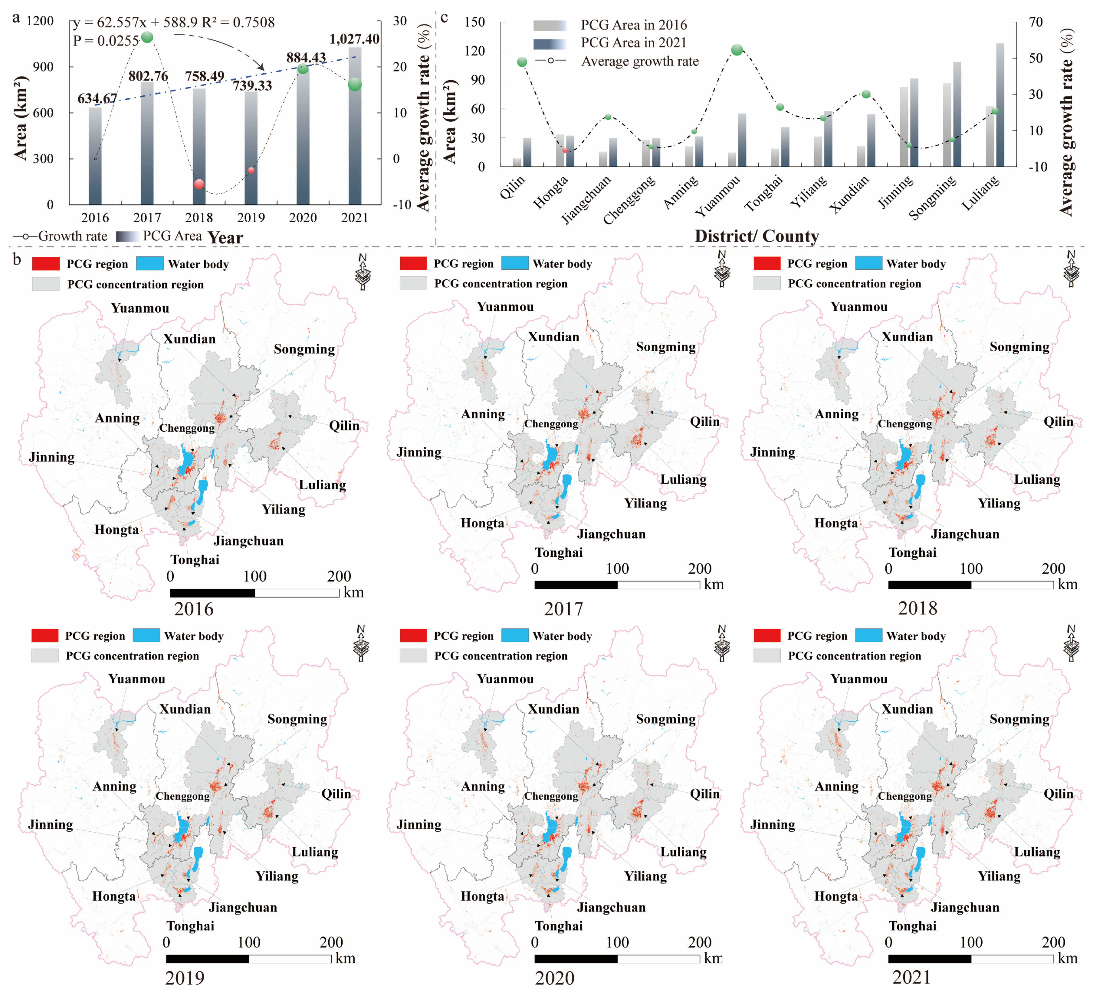
3.4. Spatiotemporal Pattern of PCG in the CYP

Figure 8 plots the PCG dynamic characteristics of CYP from 2016 to 2021. For interannual changes, the area of PCGs (Figure 8a) demonstrated an overall upwards trend in the past six years and passed the significance test with a confidence level of p < 0.05. Specifically, the PCG area increased from 634.67 km² in 2016 to 1027.40 km² in 2021, with an average growth rate and growth volume of 10.85%/yr and 65.45 km²/yr, respectively. The spatial distribution of PCG from 2016 to 2021 shows (Figure 8b) that it was mainly distributed in the central CYP, such as Luliang, Songming, and Jinning, and sporadically distributed in other regions. During the study period, the PCG area in CYP mainly demonstrated a trend of expanding along the periphery of the existing PCG area, and no new PCG gathering area was formed. Additional statistics demonstrated (Figure 8c) that the PCG increased to varying degrees in the PCG-concentrated region, except for in Hongta, where the PCG decreased slightly (−0.75%). Among these areas, Yuanmou had the fastest expansion rate, with an average annual growth rate of 54.58%, followed by Qilin (47.90%), Xundian (30.13%), Tonghai (23.06%), Luliang (20.80%), Jiangchuan (17.60%), and Yiliang (17.00%), and other regions demonstrated a relatively slow expansion trend, with an average annual growth rate of less than 10%.

4. Discussion

4.1. Influence of Feature Variables on Classification Accuracy

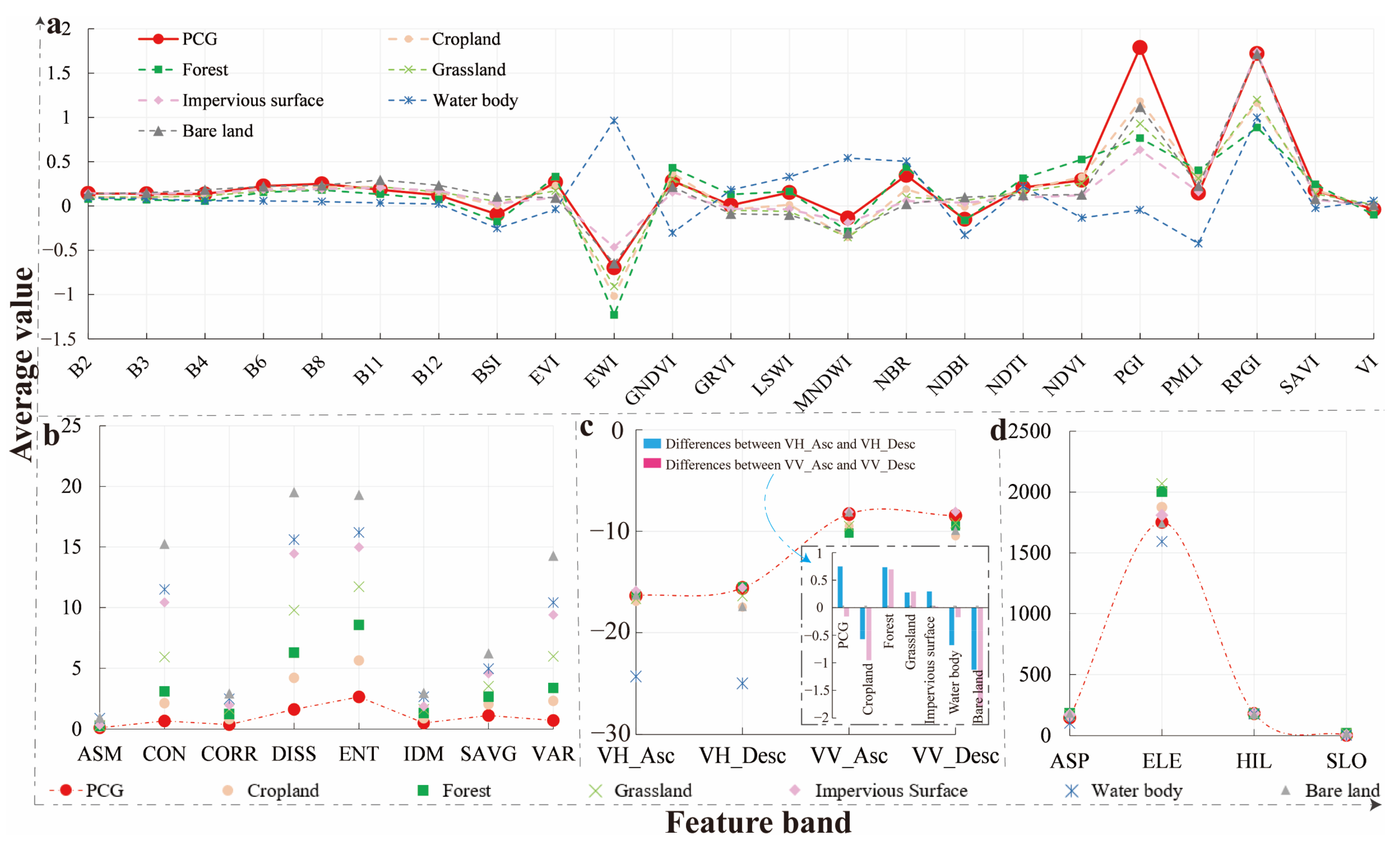
The selection of features determines whether a classification is successful, and the specific classification target is always closely related to the corresponding features. The current study screened 39 feature factors on the basis of many previous investigations (Table 2), covering multiple types of features, including spectrum, index, texture, backscatter, and terrain features, and constructed 24 feature scenarios (Figure 5a), which were combined with three machine learning classifiers to extract PCGs. The accuracy assessment results demonstrated that among all the scenarios, the S + I + B + T + Tr scenario had the highest OA and F-score in the RF, CART, and SVM classifiers (Figure 5c,d). As an artificial facility, the PCG is a layer of white plastic film covering crops, which weakens the vegetation information of the crops and gives it dual spectral characteristics that appears as soil that is covered with a small amount of vegetation and an artificial surface [74]. In numerous previous studies (e.g., Ibrahim and Gobin [46], Nemmaoui et al. [21], and Xiao et al. [45]), the spectrum and index feature tended to play the most important roles in PCG mapping tasks. However, the common phenomenon of “same objects with different spectra and different objects with the same spectrum” in optical remote sensing images is very likely to lead to the mixing and misclassification of PCGs and other land types [1]. For instance, Chen et al. [74] pointed out that the spectral features of PCGs are very similar to those of bare lands, fallow lands, and impervious surfaces, which make PCGs difficult to distinguish, especially in areas with complex land cover. Lu et al. [33] also indicated that almost all the classifiers tended to confuse and misclassify bare lands and impervious surfaces. We extracted multiple features of typical LULC types based on LULC samples and calculated the mean values of the 39 features of different LULC types (Figure 9). It demonstrated that if only the spectrum or index is used to extract the PCG, it is difficult to distinguish the PCG region from the non-PCG region except for the PGI and RPGI bands, especially the spectrum and index features of the impervious surfaces and bare lands, which are almost the same as those of the PCG. This implies that it is difficult to extract PCG using only optical features, which validates the views of Chen et al. [74] and Lu et al. [33]. In fact, the phenomenon of the poor feature heterogeneity of PCGs, impervious surfaces, and bare lands also commonly occurs in backscatter features (Figure 9b), texture features except CON, DISS, and ENT feature factors (Figure 9c), and terrain features (Figure 9d). This further revealed that it is also difficult to extract PCGs by using only a certain type of feature other than spectrum. Several recent studies have demonstrated that combining spectrum, index, backscatter, texture, and terrain features can effectively improve the PCG recognition accuracy. The present research supports the above conclusions with the following evidence: the average F-scores of the three classifiers based on the S + I + B + T + Tr scenario are 4.63% (93.59% vs. 88.96%), 29.50% (93.59% vs. 64.09%), 3.19% (93.59% vs. 90.40%), 3.07% (93.59% vs. 90.52%), 2.89% (93.59% vs. 90.70%), and 13.45% (93.59% vs. 80.14%) higher than those based on the S, B, S + I, S + B, S + T, and S + Tr scenarios, respectively (Figure 5b). This suggests that the classification accuracy of remote sensing images is affected by features, and more features will lead to a higher accuracy. It is worth noting that the F-score of the S + I + B + T + Tr scenario is 1.20% (93.59% vs. 92.39%) higher than that of the S + I + T + Tr scenario; similarly, the F-score of the S + B scenario is 1.56% (90.52% vs. 88.96%) higher than that of the S scenario, indicating that combining the backscatter features from S1 SAR is helpful for extracting PCGs, which is consistent with the previous study by Lu et al. [33].

There is also a small finding that for the S1 SAR data, the backscatter values of the ascending and descending orbits of the same LULC type have different degrees of difference, although the difference is relatively small (Figure 9c). Specifically, for the “VV” po-larization mode, the total difference of backscatter values between the ascending and descending orbits of all LULC types is 4.10, among which the difference of Bare land (1.80), Cropland (0.95), and Forest (0.70) ranks in the top three, and the difference of other LULC types are small. For the “VH” polarization mode, the total difference value of backscatter values is 4.43, among which Bare land (1.13), PCG (0.75), and Forest (0.73) have higher differences. As we know, the descending orbit refers to the movement of satellites from north to south, while the ascending orbit refers to the opposite. Different movement methods may lead to changes in observation angles and relative positions, resulting in differences in observed surface features, which will further affect the backscatter value. This indicates that when extracting backscatter features from SAR data, considering the combination of different orbits and polarization modes is helpful to identify PCGs. The high importance of VH polarization (i.e., VH_Desc, VH_Asc) in both ascending and descending orbits for PCG recognition also confirms this viewpoint (Figure 6c).

4.2. Feature Optimization Strategy

In the era of remote sensing big data, the number of available features is a huge concept. If we just increase feature dimensions endlessly, we may obtain the opposite effect. In fact, if there are lots of redundant features in the feature space, it will inevitably degrade the performance of the classifier and even reduce the classification accuracy, which is known as the “dimension disaster” [37]. Therefore, the combination of multiple features is not just a simple feature superposition but a reasonable combination. This study was the first to apply the RF-RFE method to PCG identification and optimized the optimal feature scenarios of the initial screening. The results revealed that the annual F-score improved to varying degrees after feature optimization, and the 6-year average F-score increased by 1.03% (96.63% vs. 95.60%), indicating that feature optimization had a positive impact on PCG recognition, which agrees with the findings of Chen et al. [53], He et al. [37], and Ou et al. [20]. Notably, in previous studies on feature optimization based on feature importance, the average importance was generally used as a threshold to filter feature subsets (e.g., Chen et al. [53]). To verify the feasibility of this strategy, we ranked the 6-year average importance of the features, selected feature subsets larger than the threshold that was the average importance of all features, and then used the RF classifier to extract PCGs. The evaluation results demonstrated that the F-score was 3.94% (96.63% vs. 92.69%) lower than that of this study, which demonstrated that in practical applications, a set of fixed feature subsets that were filtered only by the mean had poor generalization. Ou et al. [20] improved the optimization strategy, which iteratively optimized original features individually according to a set of feature importance ranking. In contrast, the average F-score of the current study was 5.53% (96.63 vs. 91.10%) higher than that of Ou et al. [20]. Summarizing previous studies, we believe that it is not a good idea to filter features using only the mean or a one-time ranking process because multiple experiments have demonstrated that the feature importance of the RF model changes dynamically with differences in feature combinations. Figure 6b also reveals that the optimal feature subset in different years is different, which is affected by the differences in different time-phase data; thus, it is necessary to dynamically adjust the feature subset during feature optimization. The RF-RFE strategy is to iteratively adjust the features individually based on the order of feature factors in each round. Specifically, the original feature scenario of the initial screening is used as the optimization object, the lowest-ranked feature is deleted by comparing the feature importance in the RF model of each round, the remaining features continue to participate in the next round of classification, and the lowest-ranked feature is deleted again according to the importance ranking of the new round until all the feature factors are iterated; the iteration round with the highest accuracy and corresponding best feature subset are finally selected (Figure 4). The accuracy comparison before and after the feature optimization shown in Figure 6d verify the feasibility of this strategy.

Another interesting finding was that the F-score curve of all the years fluctuated slightly before iterating to 34 rounds (6 features) and then dropped sharply with the decrease in features (Figure 6a); additionally, the top five feature factors with the highest 6-year average importance covered almost all feature types proposed in this study (Figure 6c), such as the terrain feature (ELE), the index feature (NDTI), the backscatter feature (VH_Desc, VH_Asc), and the texture feature (SAVG). The above results illustrated that too few features were extremely unfavorable for recognizing PCGs, and the PCG recognition accuracy was not absolutely affected by a certain type of feature or feature combination, which was consistent with the previous results by Aguilar et al. [39], Chen et al. [74], Lu et al. [33], and Nemmaoui et al. [21]. In general, we believe that a reasonable combination of multi-class features is an effective way to improve the recognition accuracy of PCGs.

Some additional minor findings were that the inter-category comparisons of features demonstrated that the backscatter feature outperformed the optical feature as the feature category with the highest average importance, which may be related to the special structural, textural, and dielectric properties of PCGs [2]. The intra-category comparison indicated that ELE was the feature factor with the highest average importance. This is because the spatial distribution of the PCG in CYP is affected by the economic zone and terrain that the mountains are interlaced with the dam, and is prominently agglomerated in the higher-elevation dam region, where the economy is relatively developed in the central part.

However, there are several features that were not selected for the optimal feature subset for 2016–2021, namely B4 (Red), B8 (NIR), LSWI, NDBI, SAVI, PMLI, ENT, and HIL. Thus, the average importance and cumulative frequency of these features are all 0 (Figure 6c), which indicates that these features have little contribution to the PCG identification and are invalid factors. The importance distribution trends of these features are roughly consistent with the previous study by Ou et al. [20]. Although previous experiments have confirmed that the combination of multi-source data is helpful for extracting PCG, in practice, we should fully consider the physical and chemical properties and distribution characteristics of PCG itself, and purposefully select factors with “PCG characteristics” to more effectively identify PCG. On the contrary, if we add irrelevant features aimlessly, in addition to affecting efficiency, it may also lead to the aforementioned “dimension disaster”. Therefore, the above eight ineffective features are recommended as cautious choices in subsequent PCG extraction studies.

4.3. Comparative Analysis of Classification Results and Published Products

The accuracy assessment results demonstrated that the OA and PCG’s F-score in all years were distributed above 88.00% and 95.00% (Figure 6d), respectively, indicating that the classification accuracy can meet the mapping requirements of PCGs; in addition, the visual inspection of the mapping results of PCGs in 2021 was also satisfactory (Figure 7).

We further compared the relevant products that have spatiotemporal intersections with the classification results of this study. First, for LULC classification results, there are many popular LULC products around the world, such as ESA WorldCover [75], GLOBELAND30 [76], CCI_LC [77], and MCD2Q1 [78], with spatial resolutions of 10 m, 30 m, 300 m, and 500 m, respectively. Among them, the ESA WorldCover dataset is a 2020 global 10-m land cover product jointly produced by ESA and many scientific research institutions in the world, and the OA of Asia reaches 80.7% ± 0.1%; the GLOBELAND30 product is released by the Ministry of Natural Resources of the People’s Republic of China, which has produced global LULC datasets for 2000, 2010, and 2020. It has high recognition and is widely used in various fields [76]. Considering that the relatively close spatial resolution, the ESA WorldCover and GLOBALAND30 products in 2020 were selected for visual comparison with the LULC classification results in the same year of this study (Figure 10a). At first sight, the spatial patterns of the main LULC types in three products were generally consistent. However, there are many grasslands appearing in the central and northern CYP in the GLOBELAND30 product (Figure 10(a3)), and the same phenomenon also occurs in the northern and southwestern CYP for the ESA WorldCover product (Figure 10(a2)), which is quite different from the cropland and forest land landscape dominating in CYP. In contrast, this study has a finer classification effect on forest and grassland landscapes. Additionally, a detailed comparison of several example regions demonstrated that, due to the higher pixel spatial resolution, the details of LULC are better described in the ESA WorldCover product and this study, especially for croplands and impervious surfaces (Figure 10a L I–V and E I–V). However, ESA WorldCover products have an obvious problem of misclassifying the PCG-concentrated region as bare land (Figure 10a E I and III–V). As the economic center of Yunnan Province, the land utilization rate in CYP is high, and it is unreasonable to detect so many bare lands in this product, which may be caused by similar spectral features of the PCG region and bare land [74]. Furthermore, both the ESA WorldCover and GLOBELAND30 classify various types of cropland (e.g., dry land, PCG region) into one LULC category. Admittedly, this is understandable and acceptable for macroscale research. However, as a special agricultural landscape, although the PCG belongs to the cropland, it is quite different from traditional agriculture, and it should be further distinguished when formulating regional LULC classification tasks. This study successfully separated the PCG region from croplands, which can better assist regional agricultural management and sustainable development.

The 2019 China 10-metre resolution PCG thematic data (CYP region) developed by Feng et al. [79] with the 2019 PCG extraction results of this study were also compared. Figure 10(b1,b2) shows that at the same scale, few PCG pixels were identified by Feng et al. [79]. By comparing the enlarged PCG details in several PCG-concentrated distribution zones (Figure 10b I–V) and combining them with the field aerial images of the UAVs (Figure 10b UAV I–V), the results confirmed that the PCG products extracted by Feng et al. [79] had obvious omissions (Figure 10b F I–V). Ou et al. [20] pointed out that PCGs are usually concentrated according to the terrain, spread outwards around croplands surrounding rural residential areas, and are divided by roads and rivers. Clearly, the PCG spatial pattern extracted in the present study was consistent with this view and very consistent with the S2 images (Figure 10b J I–V); it can also withstand challenges of the UAV field verification with a strong reliability. However, it should be pointed out that a few impervious surfaces and bare lands are wrongly classified as PCGs, which has been discussed in Section 4.1.

4.4. Limitations and Future Work

Regarding the data source, this study has confirmed that joint active and passive re-mote sensing data can help identify PCG. However, in December 2021, the S1B satellite mission was terminated early due to the failure of the power system unit, and the update time of the S1 GRD product supported solely by the S1A satellite will be halved, which will affect the data requirements for high-time-frequency studies. Further experiments proved that large-scale monthly or annual S1 GRD images can be successfully synthesized on GEE even using only S1A data, which makes this study unaffected by S1B satellite failure. However, for studies with higher temporal frequencies, this issue requires attention; the good news is that the latest S1C is expected to take the job of the S1B (https://www.esa.int/).

Although the method proposed in this study has been confirmed to be feasible, it requires reliable PCG samples for the detection region, which restricts the method to be applied to regions without prior knowledge in the short term; additionally, in order to meet higher application requirements, the spatial scope and temporal continuity still need to be further expanded. Combining advantages of high efficiency of the index-based method with the advantages of the high precision of the classification framework proposed in this study seems to be a promising approach to address the above problems. Consequently, future studies will try to quickly and initially screen out PCG samples through index-based methods, and use these samples as training samples for the classification framework proposed in this study to more accurately extract large-scale PCGs’; the spatial scale can even be expanded to the world. Moreover, we will more fully consider the characteristics of PGG, such as physical and chemical properties, geographic distribution, and even geophysical mechanism parameters, and try to add applicable features with superior performances to optimize the PCG recognition algorithm.

5. Conclusions

Efficient PCG mapping is essential for monitoring agricultural activities and predicting environmental impacts. This study proposed a systematic framework for the rapid extraction of large-area PCGs by combining with the GEE cloud platform with active/passive remote sensing data (i.e., S1 and S2) and conducted the first PCG spatiotemporal mapping research in CYP. The framework was developed in a progressive way and mainly included (i) the construction of different feature scenarios based on multiple feature factors; (ii) the preliminary screening of the optimal classifiers and feature scenarios; (iii) the optimization of feature scenarios to select the best feature subset; and (iv) the extraction of PCGs based on the optimum classifier and feature subset. The main findings were as follows:

(1)

The 6-year average F-score of the RF classifier in all feature scenarios was 3.77% (93.16% vs. 89.39%) and 9.26% (93.16% vs. 83.90%) higher than those of SVM and CART, respectively. Additionally, the F-score of three classifiers demonstrated an upward trend with increasing features, and the average F-score of the S + I + B + T + Tr scenario had the highest value (93.59%). The combination of the RF classifier and S + I + T + B + Tr scenario created the highest F-score of 95.60% for PCGs.

(2)

The F-score each year after feature optimization was improved to varying degrees, and the 6-year average F-score increased by 1.03% (96.63% vs. 95.60%), which proved that feature optimization had a positive impact on PCG recognition. In addition, the top five feature factors with the highest 6-year average importance were ELE, NDTI, VH_Desc, VH_Asc, and SAVG, which covered almost all the examined feature types, indicating that a reasonable combination of multiple types of features can effectively improve the recognition accuracy of PCGs.

(3)

The average F-score of PCGs extracted by the combined RF algorithm and the optimal feature subset exceeded 95.00% and passed the visual inspection from satellite images and UAV images, which indicated that the PCG spatiotemporal mapping results were reliable. From 2016 to 2021, the PCGs in CYP were prominently agglomerated in the central region, and the PCG region increased steadily, mainly demonstrating a trend of spreading out from the croplands in the PCG-concentrated region.

References

1. Lin, J.; Jin, X.; Ren, J.; Liu, J.; Liang, X.; Zhou, Y. Rapid Mapping of Large-Scale Greenhouse Based on Integrated Learning Algorithm and Google Earth Engine. Remote Sens. 2021, 13, 1245. [Google Scholar] [CrossRef]
2. Briassoulis, D.; Babou, E.; Hiskakis, M.; Scarascia, G.; Picuno, P.; Guarde, D.; Dejean, C. Review, Mapping and Analysis of the Agricultural Plastic Waste Generation and Consolidation in Europe. Waste Manag. Res. 2013, 31, 1262–1278. [Google Scholar] [CrossRef]
3. Novelli, A.; Aguilar, M.A.; Nemmaoui, A.; Aguilar, F.J.; Tarantino, E. Performance Evaluation of Object Based Greenhouse Detection from Sentinel-2 MSI and Landsat 8 OLI Data: A Case Study from Almería (Spain). Int. J. Appl. Earth Obs. Geoinf. 2016, 52, 403–411. [Google Scholar] [CrossRef] [Green Version]
4. Briassoulis, D.; Dougka, G.; Dimakogianni, D.; Vayas, I. Analysis of the Collapse of a Greenhouse with Vaulted Roof. Biosyst. Eng. 2016, 151, 495–509. [Google Scholar] [CrossRef]
5. Hasituya, H.; Chen, Z.; Wang, L.; Wu, W.; Jiang, Z.; Li, H. Monitoring Plastic-Mulched Farmland by Landsat-8 Oli Imagery Using Spectral and Textural Features. Remote Sens. 2016, 8, 353. [Google Scholar] [CrossRef] [Green Version]
6. Aguilar, M.Á.; Jiménez-Lao, R.; Nemmaoui, A.; Aguilar, F.J.; Koc-San, D.; Tarantino, E.; Chourak, M. Evaluation of the Consistency of Simultaneously Acquired Sentinel-2 and Landsat 8 Imagery on Plastic Covered Greenhouses. Remote Sens. 2020, 12, 2015. [Google Scholar] [CrossRef]
7. Katan, J. Solar heating (solarization) of soil soilborne pests. Plant Pathol. 1981, 19, 211–236. [Google Scholar] [CrossRef]
8. Picuno, P.; Sica, C.; Laviano, R.; Dimitrijević, A.; Scarascia-Mugnozza, G. Experimental Tests and Technical Characteristics of Regenerated Films from Agricultural Plastics. Polym. Degrad. Stab. 2012, 97, 1654–1661. [Google Scholar] [CrossRef]
9. Yang, D.; Chen, J.; Zhou, Y.; Chen, X.; Chen, X.; Cao, X. Mapping Plastic Greenhouse with Medium Spatial Resolution Satellite Data: Development of a New Spectral Index. ISPRS J. Photogramm. Remote Sens. 2017, 128, 47–60. [Google Scholar] [CrossRef]
10. Ou, C.; Yang, J.; Du, Z.; Liu, Y.; Feng, Q.; Zhu, D. Long-Term Mapping of a Greenhouse in a Typical Protected Agricultural Region Using Landsat Imagery and the Google Earth Engine. Remote Sens. 2020, 12, 55. [Google Scholar] [CrossRef] [Green Version]
11. Aguilar, M.A.; Bianconi, F.; Aguilar, F.J.; Fernández, I. Object-Based Greenhouse Classification from GeoEye-1 and WorldView-2 Stereo Imagery. Remote Sens. 2014, 6, 3554–3582. [Google Scholar] [CrossRef] [Green Version]
12. Wu, C.F.; Deng, J.S.; Wang, K.; Ma, L.G.; Tahmassebi, A.R.S. Object-Based Classification Approach for Greenhouse Mapping Using Landsat-8 Imagery. Int. J. Agric. Biol. Eng. 2016, 9, 79–88. [Google Scholar] [CrossRef]
13. Xiong, Y.; Zhang, Q.; Chen, X.; Bao, A.; Zhang, J.; Wang, Y. Large Scale Agricultural Plastic Mulch Detecting and Monitoring with Multi-Source Remote Sensing Data: A Case Study in Xinjiang, China. Remote Sens. 2019, 11, 2088. [Google Scholar] [CrossRef] [Green Version]
14. Zhang, P.; Du, P.; Guo, S.; Zhang, W.; Tang, P.; Chen, J.; Zheng, H. A Novel Index for Robust and Large-Scale Mapping of Plastic Greenhouse from Sentinel-2 Images. Remote Sens. Environ. 2022, 276, 113042. [Google Scholar] [CrossRef]
15. Agüera, F.; Aguilar, F.J.; Aguilar, M.A. Using Texture Analysis to Improve Per-Pixel Classification of Very High Resolution Images for Mapping Plastic Greenhouses. ISPRS J. Photogramm. Remote Sens. 2008, 63, 635–646. [Google Scholar] [CrossRef]
16. Picuno, P.; Tortora, A.; Capobianco, R.L. Analysis of Plasticulture Landscapes in Southern Italy through Remote Sensing and Solid Modelling Techniques. Landsc. Urban Plan. 2011, 100, 45–56. [Google Scholar] [CrossRef]
17. Zhang, Y.; Wang, P.; Wang, L.; Sun, G.; Zhao, J.; Zhang, H.; Du, N. The Influence of Facility Agriculture Production on Phthalate Esters Distribution in Black Soils of Northeast China. Sci. Total Environ. 2015, 506–507, 118–125. [Google Scholar] [CrossRef]
18. Ge, D.; Wang, Z.; Tu, S.; Long, H.; Yan, H.; Sun, D.; Qiao, W. Coupling Analysis of Greenhouse-Led Farmland Transition and Rural Transformation Development in China’s Traditional Farming Area: A Case of Qingzhou City. Land Use Policy 2019, 86, 113–125. [Google Scholar] [CrossRef]
19. He, F.; Ma, C. Development and Strategy of Facility Agriculture in China. Chin. Agric. Sci. Bull. 2007, 23, 462–465. [Google Scholar]
20. Ou, C.; Yang, J.; Du, Z.; Zhang, T.; Niu, B.; Feng, Q.; Liu, Y.; Zhu, D. Landsat-Derived Annual Maps of Agricultural Greenhouse in Shandong Province, China from 1989 to 2018. Remote Sens. 2021, 13, 4830. [Google Scholar] [CrossRef]
21. Nemmaoui, A.; Aguilar, M.A.; Aguilar, F.J.; Novelli, A.; Lorca, A.G. Greenhouse Crop Identification from Multi-Temporal Multi-Sensor Satellite Imagery Using Object-Based Approach: A Case Study from Almería (Spain). Remote Sens. 2018, 10, 1751. [Google Scholar] [CrossRef] [Green Version]
22. Matton, N.; Canto, G.S.; Waldner, F.; Valero, S.; Morin, D.; Inglada, J.; Arias, M.; Bontemps, S.; Koetz, B.; Defourny, P. An Automated Method for Annual Cropland Mapping along the Season for Various Globally-Distributed Agrosystems Using High Spatial and Temporal Resolution Time Series. Remote Sens. 2015, 7, 13208–13232. [Google Scholar] [CrossRef] [Green Version]
23. Aguilar, M.A.; Vallario, A.; Aguilar, F.J.; Lorca, A.G.; Parente, C. Object-Based Greenhouse Horticultural Crop Identification from Multi-Temporal Satellite Imagery: A Case Study in Almeria, Spain. Remote Sens. 2015, 7, 7378–7401. [Google Scholar] [CrossRef] [Green Version]
24. González-Yebra, Ó.; Aguilar, M.A.; Nemmaoui, A.; Aguilar, F.J. Methodological Proposal to Assess Plastic Greenhouses Land Cover Change from the Combination of Archival Aerial Orthoimages and Landsat Data. Biosyst. Eng. 2018, 175, 36–51. [Google Scholar] [CrossRef]
25. Lu, L.; Di, L.; Ye, Y. A Decision-Tree Classifier for Extracting Transparent Plastic-Mulched Landcover from Landsat-5 TM Images. IEEE J. Sel. Top. Appl. Earth Obs. Remote Sens. 2014, 7, 4548–4558. [Google Scholar] [CrossRef]
26. Novelli, A.; Tarantino, E. Combining Ad Hoc Spectral Indices Based on LANDSAT-8 OLI/TIRS Sensor Data for the Detection of Plastic Cover Vineyard. Remote Sens. Lett. 2015, 6, 933–941. [Google Scholar] [CrossRef]
27. Hasituya; Chen, Z.; Wang, L.; Liu, J. Selecting Appropriate Spatial Scale for Mapping Plastic-Mulched Farmland with Satellite Remote Sensing Imagery. Remote Sens. 2017, 9, 265. [Google Scholar] [CrossRef] [Green Version]
28. Levin, N.; Lugassi, R.; Ramon, U.; Braun, O.; Ben-Dor, E. Remote Sensing as a Tool for Monitoring Plasticulture in Agricultural Landscapes. Int. J. Remote Sens. 2007, 28, 183–202. [Google Scholar] [CrossRef]
29. Carvajal, F.; Agüera, F.; Aguilar, F.J.; Aguilar, M.A. Relationship between Atmospheric Corrections and Training-Site Strategy with Respect to Accuracy of Greenhouse Detection Process from Very High Resolution Imagery. Int. J. Remote Sens. 2011, 31, 2977–2994. [Google Scholar] [CrossRef]
30. Koc-San, D. Evaluation of Different Classification Techniques for the Detection of Glass and Plastic Greenhouses from WorldView-2 Satellite Imagery. J. Appl. Remote Sens. 2013, 7, 073553. [Google Scholar] [CrossRef]
31. Balcik, F.B.; Senel, G.; Goksel, C. Greenhouse Mapping Using Object Based Classification and Sentinel-2 Satellite Imagery. In Proceedings of the 2019 8th International Conference on Agro-Geoinformatics (Agro-Geoinformatics), Istanbul, Turkey, 16–19 July 2019. [Google Scholar] [CrossRef]
32. Jiménez-Lao, R.; Aguilar, F.J.; Nemmaoui, A.; Aguilar, M.A. Remote Sensing of Agricultural Greenhouses and Plastic-Mulched Farmland: An Analysis of Worldwide Research. Remote Sens. 2020, 12, 2649. [Google Scholar] [CrossRef]
33. Lu, L.; Tao, Y.; Di, L. Object-Based Plastic-Mulched Landcover Extraction Using Integrated Sentinel-1 and Sentinel-2 Data. Remote Sens. 2018, 10, 1820. [Google Scholar] [CrossRef] [Green Version]
34. Qi, Z.; Yeh, A.G.O.; Li, X.; Lin, Z. A Novel Algorithm for Land Use and Land Cover Classification Using RADARSAT-2 Polarimetric SAR Data. Remote Sens. Environ. 2012, 118, 21–39. [Google Scholar] [CrossRef]
35. Veloso, A.; Mermoz, S.; Bouvet, A.; Le Toan, T.; Planells, M.; Dejoux, J.F.; Ceschia, E. Understanding the Temporal Behavior of Crops Using Sentinel-1 and Sentinel-2-like Data for Agricultural Applications. Remote Sens. Environ. 2017, 199, 415–426. [Google Scholar] [CrossRef]
36. Ma, L.; Li, M.; Ma, X.; Cheng, L.; Du, P.; Liu, Y. A Review of Supervised Object-Based Land-Cover Image Classification. ISPRS J. Photogramm. Remote Sens. 2017, 130, 277–293. [Google Scholar] [CrossRef]
37. He, Z.; Zhang, M.; Wu, B.; Xing, Q. Extraction of Summer Crop in Jiangsu Based on Google Earth Engine. J. Geo-Inf. Sci. 2019, 21, 752–766. [Google Scholar] [CrossRef]
38. Ma, A.; Chen, D.; Zhong, Y.; Zheng, Z.; Zhang, L. National-Scale Greenhouse Mapping for High Spatial Resolution Remote Sensing Imagery Using a Dense Object Dual-Task Deep Learning Framework: A Case Study of China. ISPRS J. Photogramm. Remote Sens. 2021, 181, 279–294. [Google Scholar] [CrossRef]
39. Aguilar, M.A.; Nemmaoui, A.; Novelli, A.; Aguilar, F.J.; Lorca, A.G. Object-Based Greenhouse Mapping Using Very High Resolution Satellite Data and Landsat 8 Time Series. Remote Sens. 2016, 8, 513. [Google Scholar] [CrossRef] [Green Version]
40. Li, J.; Wang, J.; Zhang, J.; Liu, C.; He, S.; Liu, L. Growing-Season Vegetation Coverage Patterns and Driving Factors in the China-Myanmar Economic Corridor Based on Google Earth Engine and Geographic Detector. Ecol. Indic. 2022, 136, 108620. [Google Scholar] [CrossRef]
41. Gorelick, N.; Hancher, M.; Dixon, M.; Ilyushchenko, S.; Thau, D.; Moore, R. Google Earth Engine: Planetary-Scale Geospatial Analysis for Everyone. Remote Sens. Environ. 2017, 202, 18–27. [Google Scholar] [CrossRef]
42. Shelestov, A.; Lavreniuk, M.; Kussul, N.; Novikov, A.; Skakun, S. Exploring Google Earth Engine Platform for Big Data Processing: Classification of Multi-Temporal Satellite Imagery for Crop Mapping. Front. Earth Sci. 2017, 5, 17. [Google Scholar] [CrossRef] [Green Version]
43. Yu, Y.; Shen, Y.; Wang, J.; Wei, Y.; Liu, Z. Simulation and Mapping of Drought and Soil Erosion in Central Yunnan Province, China. Adv. Sp. Res. 2021, 68, 4556–4572. [Google Scholar] [CrossRef]
44. Nong, L.; Wang, J.; Yu, Y. Research on Ecological Environment Quality in Central Yunnan Based on MRSEI Model. J. Ecol. Rural Environ. 2021, 37, 972–982. [Google Scholar]
45. Xiao, W.; Xu, S.; He, T. Mapping Paddy Rice with Sentinel-1/2 and Phenology-, Object-Based Algorithm—A Implementation in Hangjiahu Plain in China Using Gee Platform. Remote Sens. 2021, 13, 990. [Google Scholar] [CrossRef]
46. Ibrahim, E.; Gobin, A. Sentinel-2 Recognition of Uncovered and Plastic Covered Agricultural Soil. Remote Sens. 2021, 13, 4195. [Google Scholar] [CrossRef]
47. Liu, C.; Li, W.; Zhu, G.; Zhou, H.; Yan, H.; Xue, P. Land Use/Land Cover Changes and Their Driving Factors in the Northeastern Tibetan Plateau Based on Geographical Detectors and Google Earth Engine: A Case Study in Gannan Prefecture. Remote Sens. 2020, 12, 3139. [Google Scholar] [CrossRef]
48. Song, C.; Woodcock, C.E.; Seto, K.C.; Lenney, M.P.; Macomber, S.A. Classification and Change Detection Using Landsat TM Data. Remote Sens. Environ. 2001, 75, 230–244. [Google Scholar] [CrossRef]
49. Farr, T.G.; Rosen, P.A.; Caro, E.; Crippen, R.; Duren, R. The Shuttle Radar Topography Mission. Rev. Geophys. 2007, 45, 65–77. [Google Scholar] [CrossRef] [Green Version]
50. Chen, Y.; Wang, J. Ecological Security Early-Warning in Central Yunnan Province, China, Based on the Gray Model. Ecol. Indic. 2020, 111, 106000. [Google Scholar] [CrossRef]
51. Fernández-Buces, N.; Siebe, C.; Cram, S.; Palacio, J.L. Mapping Soil Salinity Using a Combined Spectral Response Index for Bare Soil and Vegetation: A Case Study in the Former Lake Texcoco, Mexico. J. Arid Environ. 2006, 65, 644–667. [Google Scholar] [CrossRef]
52. Tassi, A.; Vizzari, M. Object-Oriented Lulc Classification in Google Earth Engine Combining Snic, Glcm, and Machine Learning Algorithms. Remote Sens. 2020, 12, 3776. [Google Scholar] [CrossRef]
53. Chen, X.; Yang, K.; Wang, J. Extraction of Impervious Surface in Mountainous City Combined with Sentinel Images and Feature Optimization. Softw. Guid. 2022, 21, 214–219. [Google Scholar]
54. Zhang, H.; Lin, H.; Li, Y.; Zhang, Y.; Fang, C. Mapping Urban Impervious Surface with Dual-Polarimetric SAR Data: An Improved Method. Landsc. Urban Plan. 2016, 151, 55–63. [Google Scholar] [CrossRef]
55. Roy, P.S.; Sharma, K.P.; Jain, A. Stratification of Density in Dry Deciduous Forest Using Satellite Remote Sensing Digital Data—An Approach Based on Spectral Indices. J. Biosci. 1996, 21, 723–734. [Google Scholar] [CrossRef]
56. He, Y.; Zhang, B.; Ma, C. The Impact of Dynamic Change of Cropland on Grain Production in Jilin. J. Geogr. Sci. 2004, 14, 56–62. [Google Scholar] [CrossRef]
57. Jiang, Z.; Huete, A.R.; Didan, K.; Miura, T. Development of a Two-Band Enhanced Vegetation Index without a Blue Band. Remote Sens. Environ. 2008, 112, 3833–3845. [Google Scholar] [CrossRef]
58. Wang, Z.; Zhang, Q.; Qian, J.; Xiao, X. Greenhouse Extraction Based on the Enhanced Water Index—A Case Study in Jiangmen of Guangdong. J. Integr. Technol. 2017, 6, 11–21. [Google Scholar]
59. Rouse, J.; Haas, R.; Schell, J.; Deering, D. Monitoring Vegetation Systems in the Great Plains with ERTS. NASA Spec. Publ. 1974, 351, 309. [Google Scholar]
60. Phadikar, S.; Goswami, J. Vegetation Indices Based Segmentation for Automatic Classification of Brown Spot and Blast Diseases of Rice. In Proceedings of the 2016 3rd International Conference on Recent Advances in Information Technology (RAIT), Dhanbad, India, 3–5 March 2016; pp. 284–289. [Google Scholar] [CrossRef]
61. Khadanga, G.; Jain, K. Tree Census Using Circular Hough Transform and GRVI. Procedia Comput. Sci. 2020, 171, 389–394. [Google Scholar] [CrossRef]
62. Chandrasekar, K.; Sesha Sai, M.V.R.; Roy, P.S.; Dwevedi, R.S. Land Surface Water Index (LSWI) Response to Rainfall and NDVI Using the MODIS Vegetation Index Product. Int. J. Remote Sens. 2010, 31, 3987–4005. [Google Scholar] [CrossRef]
63. Xu, H. A Study on Information Extraction of Water Body with the Modified Normalized Difference Water Index (MNDWI). J. Remote Sens. 2005, 9, 589–595. [Google Scholar]
64. Picotte, J.J.; Peterson, B.; Meier, G.; Howard, S.M. 1984–2010 Trends in Fire Burn Severity and Area for the Conterminous US. Int. J. Wildl. Fire 2016, 25, 413–420. [Google Scholar] [CrossRef]
65. Aziz, M.A. Applying the Normalized Difference Built-Up Index to the Fayoum Oasis, Egypt (1984–2013). Remote Sens. GIS Appl. Nat. Resour. Popul. 2014, 2, 53–66. [Google Scholar]
66. Huete, A.R. A Soil-Adjusted Vegetation Index (SAVI). Remote Sens. Environ. 1988, 25, 295–309. [Google Scholar] [CrossRef]
67. Breiman, L.; Friedman, J.H.; Olshen, R.A.; Stone, C.J. Classification and Regression Trees. Biometrics 1984, 40, 874. [Google Scholar]
68. Breiman, L.; Last, M.; Rice, J. Random Forests: Finding Quasars. In Statistical Challenges in Astronomy; Springer: New York, NY, USA, 2003; pp. 243–254. [Google Scholar] [CrossRef]
69. Cortes, C.; Vapnik, V. Support-Vector Networks. Mach. Learn. 1995, 20, 273–297. [Google Scholar] [CrossRef]
70. Guyon, I.; Weston, J.; Barnhill, S.; Vapnik, V. Gene Selection for Cancer Classification Using Support Vector Machines. Mach. Learn. 2002, 46, 389–422. [Google Scholar] [CrossRef]
71. Darst, B.F.; Malecki, K.C.; Engelman, C.D. Using Recursive Feature Elimination in Random Forest to Account for Correlated Variables in High Dimensional Data. BMC Genet. 2018, 19, 65. [Google Scholar] [CrossRef] [Green Version]
72. Grabska, E.; Frantz, D.; Ostapowicz, K. Evaluation of Machine Learning Algorithms for Forest Stand Species Mapping Using Sentinel-2 Imagery and Environmental Data in the Polish Carpathians. Remote Sens. Environ. 2020, 251, 112103. [Google Scholar] [CrossRef]
73. Gregorutti, B.; Michel, B.; Saint-Pierre, P. Correlation and Variable Importance in Random Forests. Stat. Comput. 2017, 27, 659–678. [Google Scholar] [CrossRef] [Green Version]
74. Chen, J.; Shen, R.; Li, B.; Ti, C.; Yan, X.; Zhou, M.; Wang, S. The Development of Plastic Greenhouse Index Based on Logistic Regression Analysis. Remote Sens. Nat. Resour. 2019, 31, 43–50. [Google Scholar]
75. Zanaga, D.; Van De Kerchove, R.; De Keersmaecker, W.; Souverijns, N.; Brockmann, C.; Quast, R.; Wevers, J.; Grosu, A.; Paccini, A.; Vergnaud, S. ESA WorldCover 10 m 2020 V100. 2021. Available online: https://zenodo.org/record/5571936 (accessed on 28 September 2021).
76. Li, J.; Wang, J.; Zhang, J.; Zhang, J.; Kong, H. Dynamic Changes of Vegetation Coverage in China-Myanmar Economic Corridor over the Past 20 Years. Int. J. Appl. Earth Obs. Geoinf. 2021, 102, 102378. [Google Scholar] [CrossRef]
77. Bontemps, S.; Boettcher, M.; Brockmann, C.; Kirches, G.; Lamarche, C.; Radoux, J.; Santoro, M.; Van Bogaert, E.; Wegmüller, U.; Herold, M.; et al. Multi-Year Global Land Cover Mapping at 300 M and Characterization for Climate Modelling: Achievements of the Land Cover Component of the ESA Climate Change Initiative. Int. Arch. Photogramm. Remote Sens. Spat. Inf. Sci.-ISPRS Arch. 2015, 40, 323–328. [Google Scholar] [CrossRef] [Green Version]
78. Friedl, M.A.; Sulla-Menashe, D.; Tan, B.; Schneider, A.; Ramankutty, N.; Sibley, A.; Huang, X. MODIS Collection 5 Global Land Cover: Algorithm Refinements and Characterization of New Datasets. Remote Sens. Environ. 2010, 114, 168–182. [Google Scholar] [CrossRef]
79. Feng, Q.; Niu, B.; Zhu, D.; Yao, X.; Liu, Y. A Dataset of Remote Sensing-Based Classification for Agricultural Plastic Greenhouses in China in 2019. China Sci. Data 2021, 6, 153–170. [Google Scholar] [CrossRef] [PubMed] [Green Version]
Figure 1. Central Yunnan Province (CYP) region: (a) location; (b) administrative divisions; (c) sentinel-2 (S2) images in the plastic-covered greenhouses (PCGs) region; (d) unmanned aerial vehicle (UAV) images in the PCGs region.
Remotesensing 15 03287 g001
Figure 2. LULC Samples: (a) final LULC sample library formed from field-collected LULC samples (larger points) and the visually expanded samples (smaller points); (b) the number of various LULC samples from 2016 to 2021.
Remotesensing 15 03287 g002
Figure 3. The research flowchart of the current study.
Remotesensing 15 03287 g003
Figure 4. Recursive feature elimination process based on random forest algorithm, where i represents the total number of the feature factor.
Remotesensing 15 03287 g004
Figure 5. Accuracy evaluation of the combination of feature scenarios and classifiers: (a) feature scenarios, where S, B, I, T, and Tr represent spectrum, backscatter, index, texture, and terrain features, respectively; (b) average accuracy for different feature scenarios; (c) OA of different classifiers based on different feature scenarios; (d) F-score of different classifiers based on different feature scenarios.
Remotesensing 15 03287 g005
Figure 6. Feature optimization, importance analysis, and accuracy assessment: (a) the changes of the F-score curve with the increase in iteration rounds in different years; (b) the feature subsets corresponding to the iteration round with the highest F-score; (c) the 6-year average importance and cumulative frequency of each feature in the best feature subsets; (d) accuracy comparison before and after feature optimization.
Remotesensing 15 03287 g006
Figure 7. Visual inspection by comparing the LULC classification results in 2021 with S2 images and UAV images. Note: small letters (a–f) represent six typical regions where PCGs were concentrated that we have checked.
Remotesensing 15 03287 g007
Figure 8. Spatiotemporal features of PCGs extracted in CYP from 2016 to 2021: (a) temporal changes in PCGs; (b) annual spatial distribution of PCGs; (c) PCG changes in regions where they are concentrated.
Remotesensing 15 03287 g008
Figure 9. Features of typical LULC types: (a) spectrum and index features; (b) texture features; (c) backscatter features and backscatter difference between different orbits for the same LULC type; (d) terrain features.
Remotesensing 15 03287 g009
Figure 10. Visual comparison of LULC/PCG datasets produced by the current study with (a) GLOBALAND30 products and ESA WorldCover products; (b) PCG datasets published by Feng et al. [79]. I–V are demonstration zones for further detailed comparison.
Remotesensing 15 03287 g010