Article

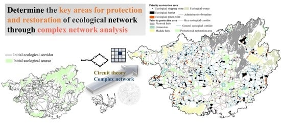
How to Optimize High-Value GEP Areas to Identify Key Areas for Protection and Restoration: The Integration of Ecology and Complex Networks

1
College of Forestry, Guangxi University, Nanning 530004, China
2
State Key Laboratory of Urban and Regional Ecology, Research Center for Eco-Environmental Sciences, Chinese Academy of Sciences, Beijing 100085, China
3
School of Mechanical Engineering, Guangxi University, Nanning 530004, China
4
Institute of Ecological Protection and Restoration, Chinese Academy of Forestry (CAF), Beijing 100091, China
5
International Center for Climate and Global Change Research, College of Forestry, Wildlife and Environment, Auburn University, Auburn, AL 36849, USA
*
Author to whom correspondence should be addressed.
Remote Sens. 2023, 15(13), 3420; https://doi.org/10.3390/rs15133420
Submission received: 29 May 2023 / Revised: 28 June 2023 / Accepted: 3 July 2023 / Published: 6 July 2023
(This article belongs to the Special Issue Applications of Remote Sensing in Spatial Ecology)

Abstract

:
Identifying and protecting key sites of ecological assets and improving spatial connectivity and accessibility are important measures taken to protect ecological diversity. This study takes Guangxi as the research area. Based on the gross ecosystem product (GEP), the ecological source is identified, and the initial ecological network (EN) is constructed by identifying the ecological corridor with the minimum cumulative resistance model. The internal defects of the initial ecological network are extracted using the circuit theory, the priority areas for restoration and protection with clear spatial positions are determined according to the complex network analysis, and the network’s performance before and after optimization is comprehensively evaluated. The results show that 456 initial ecological sources and 1219 ecological corridors have been identified, forming the initial ecological network of Guangxi. Based on the circuit theory, 168 ecological barriers, 83 ecological pinch points, and 71 ecological stepping stones were extracted for network optimization. After optimizing the ecological network, there are 778 ecological sources with a total area of 73,950.56 km2 and 2078 ecological corridors with a total length of 23,922.07 km. The GEP of the optimized structure is 13.33% higher than that of the non-optimized structure. The priority areas for protection are distributed in a large area, and the attached GEP reaches USD 118 billion, accounting for 72% of the total GEP attached to the optimized ecological source area. The priority areas for restoration are scattered in small patches, with a GEP of USD 19.27 billion. The robustness and connectivity of the optimized ecological network have been improved obviously. This study attempts to identify key sites of ecological assets and the priority regions for restoration and conservation using genuine geographical location and reference materials for regional ecological network optimization and implementation.

Graphical Abstract

1. Introduction

According to statistics, about 28% of species are at risk of disappearing forever. This state poses a serious threat to the health and sustainable development of the global ecosystem [1]. Studies have shown that biodiversity is a necessary factor to maintain the function and adaptability of ecosystems [2]. However, with the expansion of human activities, current global biodiversity is facing enormous pressure, and many species are on the verge of extinction; thus, it is particularly important to protect biodiversity [3].
Protected areas are an important means to maintain biodiversity, and ecological connectivity is one of the core elements of protected areas [4,5,6]. China has established nearly 100,000 protected areas, giving priority to ensuring the safety of ecosystems and biodiversity [7], such as problems in the restoration of Asian tiger population and forest land protection [8,9,10]; the protected areas are isolated, and species cannot be effectively exchanged and migrated. The ecological network is regarded as an example of protected area construction, which can effectively reduce landscape fragmentation and further promote the protection of threatened habitats and internal biota [11,12]. Therefore, the ecological network has become one of the most important ways to protect the ecosystem and maintain biodiversity. Ecological network theory originated from the landscape ecological planning method, and has become a mature research paradigm: ecological source identification–resistance surface construction–corridor extraction [13,14,15]. Among them, the identification of ecological sources includes direct identification, landscape spatial pattern analysis, and ecosystem service importance evaluation. The ecological corridor is the skeleton of the ecological network, which can promote the exchange and migration of species between different patches, and promote the exchange of species genes.
A good spatial structure promotes the ecological process, thus changing the spatial structure and realizing a virtuous circle [16,17,18]. Different species, groups and environments in the ecosystem are connected together, forming interdependent and interactive relationships. Drawing lessons from the circuit theory in physics, this paper analyzes the elements of analog circuit theory: current, voltage, resistance, circuit, and network. For example, the interaction of the ecosystem can be analogized as the connection and interaction in the circuit; we aim to understand the dynamics and stability of the ecosystem more deeply. The topological properties of complex network theory have been widely used in analyzing the structures of ecological space networks and the state of elements in the network, and a series of network optimization strategies have been put forward [19,20]. However, these studies ignore the importance of spatial location to the ecological network, and ignore the influence of the internal defects of the ecological network on its function and effectiveness. The existing research often focuses on the network construction and optimization of the ecosystem service’s supply and demand (and landscape spatial structure), but there is little research on identifying and optimizing high-value key areas for protection and restoration. Therefore, this study attempts to expand the application of the ecological network and solve the shortcomings of previous studies on ecological network optimization. In our work, the priority areas for restoration and protection (with clear spatial positions) are determined by applying circuit theory and calculating the connectivity of connected modules. The optimization strategy, considering spatial location, can provide more support for actual decision-making than the abstract optimization strategy. Secondly, the optimization effect of the ecological network is verified and evaluated through network robustness in complex network analysis.
Stimulating the enthusiasm and initiative of ecological protectors is the key to effectively protecting biodiversity [21,22]. This is of great significance for achieving global goals, such as the United Nations’ sustainable development goals and those of the Kunming–Montreal global biodiversity framework. However, because the effect of protecting the ecological environment is often abstract, the public and some reserve managers lack specific understanding of the benefits of ecological protection, which seriously restricts the pace of ecological improvement [23,24]. Therefore, evaluating the value of products and services provided by ecosystem services is one of the most important means we have of protecting biodiversity. In 2013, Ouyang Zhiyun was the first to put forward the concept of gross ecosystem product (also known as ecosystem service value, GEP) [25]. GEP is regarded as the value of products and services provided by the ecosystem for human welfare and sustainable economic and social development in a certain period and region [26]. China scholars have carried out GEP research in many administrative units [26,27,28]. In other countries, such as Britain and Australia, research on ecosystem value accounting has also been widely carried out [29,30]. Through the evaluation of GEP, we can re-recognize the value of ecological resources, reveal the key areas for ecological environmental protection, and increase the public’s understanding and support for the ecological environment, so as to help them to realize that protecting and restoring the ecological environment will directly promote economic prosperity and sustainable development.
Guangxi is an important province in South China with obvious ecological advantages; it not only produces huge ecological benefits locally, but also plays a vital role in maintaining the ecological security of neighboring provinces and even East Asia. At present, there are still few studies identifying high-value key areas in Guangxi, and the dominant studies concern only ecological security and ecological security pattern construction [31,32]. However, optimizing regional spatial connections will not only help to protect biodiversity, but will also promote the transformation of ecological advantages into economic advantages, and promote the economic development of Guangxi. Therefore, this study takes Guangxi, China as a case study area, and develops a comprehensive method to identify and optimize high-value key areas and their spatial relations, and provide methodological references for their areas. The main objectives of this study are as follows: firstly, to quantify and identify the spatial scope of the key areas of GEP in Guangxi in 2020; secondly, according to complex network and circuit theory, to determine the priority areas for ecosystem restoration and protection, and formulate an optimization scheme; and thirdly, to use the complex network analysis index and robustness index to analyze the ecological network before and after optimization, and evaluate the effect of the optimization scheme.

2. Study Area and Data Sources
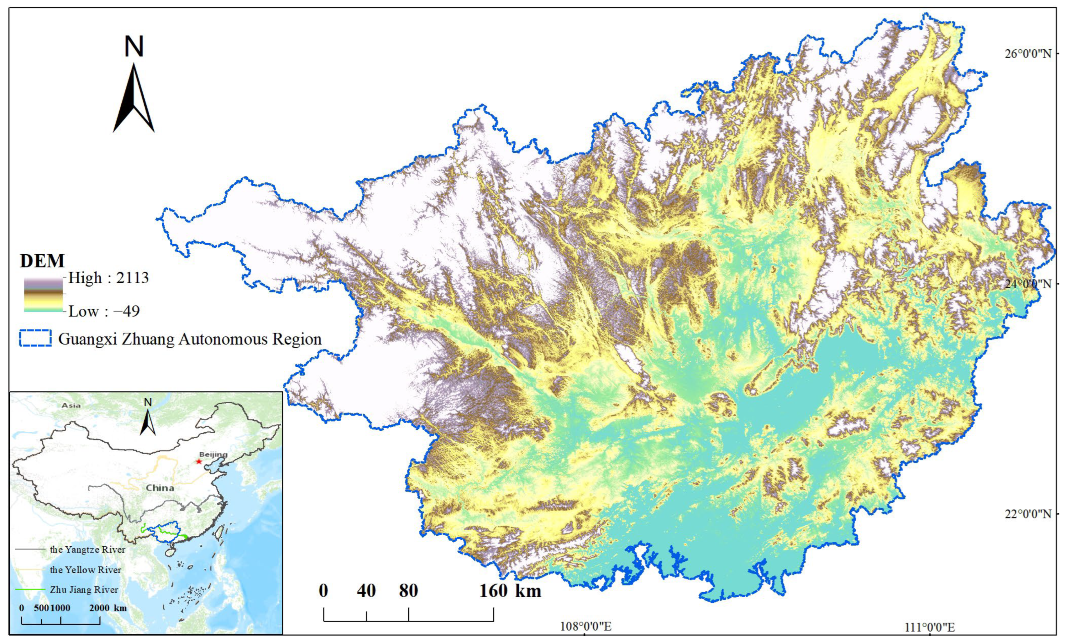
2.1. Study Area

Guangxi is a province in South China which is situated between 26~21.7°N and 104.5~112°E (Figure 1). Guangxi has a subtropical monsoon climate, with 1937 mm of rainfall on average. The area’s entire land area is 236,700 km2. Guangxi has connections to Hunan in the northeast and Guangdong in the east. It is situated on the southeast margin of the Yunnan-Guizhou Plateau in the second step of China, bordering Yunnan to the west and Guizhou to the northwest. Guangxi is a Chinese region located along the coast, bordered by rivers and the coast, with the Beibu Gulf to the south and Hainan Island across the sea. The mainland coastline is about 1500 km long. Guangxi is bordered by Vietnam in the southwest, which is an important channel for China’s east–west and north–south exchanges, as well as an important section connecting Southeast Asia. Guangxi’s karst landform is widely distributed, with intricate basins and hills. Guangxi has a wide variety of ecological resources, rich forest resources, and a high-quality natural environment. Most of the rivers in China flow from the northwest to southeast along with the terrain. As of the end of 2020, Guangxi’s gross domestic product (GDP) was USD 321.23 billion.

2.2. Data Sources

The data used in this study mainly include geospatial data and socioeconomic data. Land use data (LULC) come from NASA, with a spatial resolution of 250 m. The land types are divided into six categories: construction land, cultivated land, woodland, grassland, water, and shrub. Administrative division data, normalized difference vegetation index (NDVI) data, and digital elevation model (DEM) data with a resolution of 30 m are from the Academy of Sciences of China Resources and Environmental Science Data Center (https://www.resdc.cn/, accessed on 1 September 2022). NDVI data are a vegetation index dataset based on the vegetation index data of SPOT/VEGATION PROBA-V1km products and generated using the maximum value synthesis method. Soil data come from the National Soil Information Service Platform (http://www.soilinfo.cn/, accessed on 15 December 2021). Meteorological data, such as precipitation and evapotranspiration, come from the Monitoring Center of China Environmental Protection Administration (http://www.cnemc.cn/, accessed on 15 December 2021). Night lighting data come from the National Environmental Information Center (http://www.ngdc.noaa.gov, accessed on 10 September 2022). Population density data come from World POP Datasets (https://www.worldpop.org/, accessed on 10 September 2022). Road and water data come from the National Basic Geographic Information Center (http://www.ngcc.cn/ngcc/, accessed on 10 September 2022). Social and economic data come from the Guangxi Statistical Yearbook and the Guangxi National Economic and Social Development Statistical Bulletin [33].

3. Methods

The four steps that make up this study’s research framework are as follows: (1) identifying ecological sources using high values of GEP; (2) based on spatial principal component analysis (SPCA), constructing the minimum cumulative resistance surface; (3) identifying and improving the internal defects of the initial ecological network, accomplishing network optimization, and determining the priority areas for restoration and protection; and (4) comparing and analyzing the ecological network structure and network anti-attack ability before and after optimization, and evaluating the optimization effect. Figure 2 depicts the study’s technical flow.

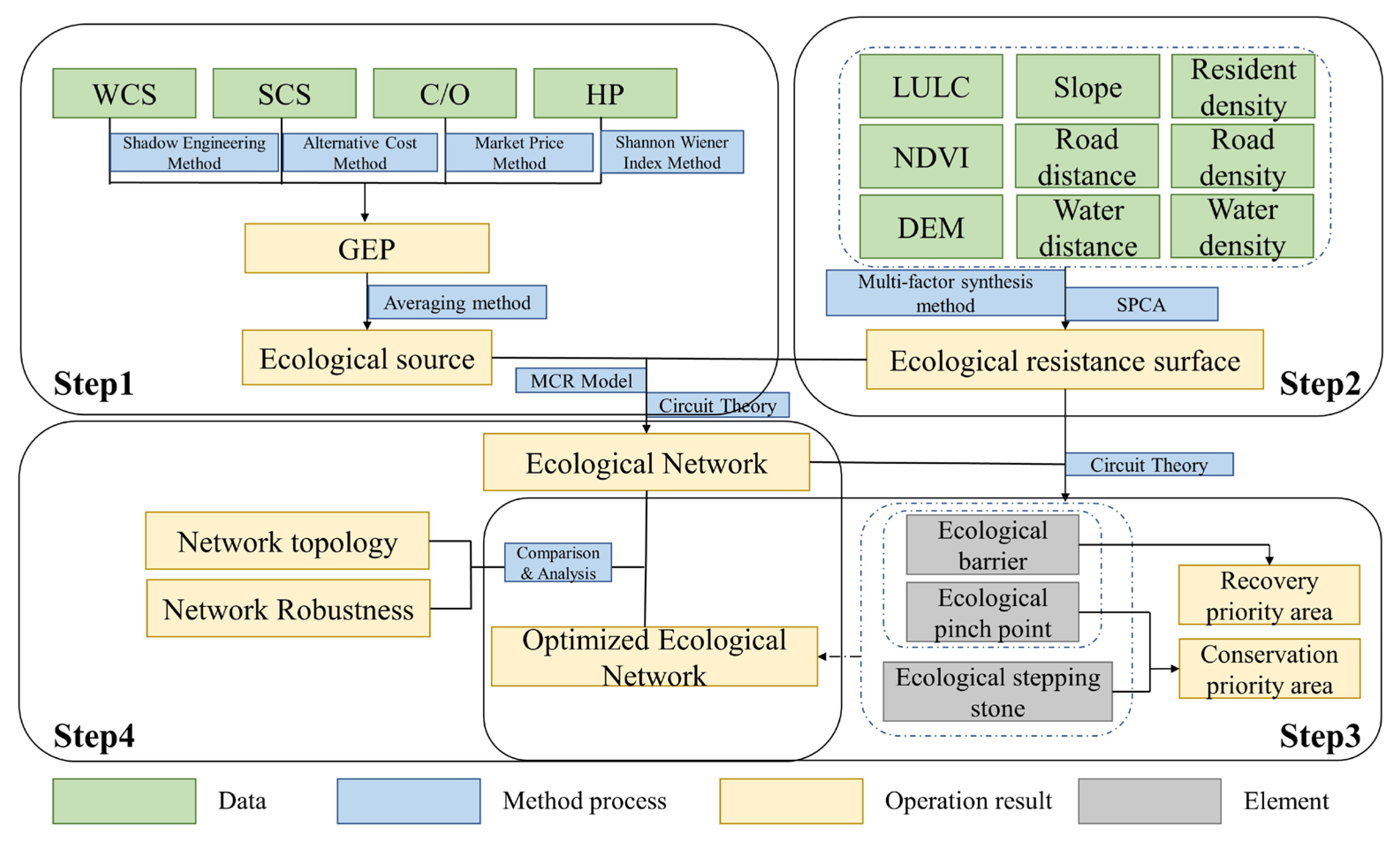
3.1. Ecological Network (EN) Construction

3.1.1. Selection of Ecological Source

Defining the function and value of the ecosystem is the basis of effectively protecting ecological resources and biodiversity. According to the geographical and environmental characteristics of Guangxi, we use four indicators to quantify the gross ecosystem product (GEP): the water conservation service (WCS), soil conservation service (SCS), carbon sequestration and oxygen release service (C/O) and habitat provision (HP). These indicators help us to understand the characteristics and protection measures of the Guangxi ecosystem, which is the basis for identifying ecological sources and ecological corridors as the study area [34] (Table 1).
Based on the theory of environmental economics, we use the shadow engineering method, replacement market method, market price method and Shannon–Wiener index method to evaluate the value of ecosystem services. The shadow engineering method is a method to measure and estimate the social and economic value of environmental resources and functions. It analyzes the supply and demand of environmental resources and their contribution to human welfare, so as to determine their economic value. The replacement market method is a method used to infer the potential economic value of non-market resources, which is based on the price and demand of similar resources or substitutes on the market. The market price method evaluates the value of resources and ecosystem services according to market behaviors and transactions. The Shannon–Wiener index rule applies the concept of information theory to evaluate biodiversity and species richness. Together, these methods help us to better understand and manage the important value of the environment and ecosystem.

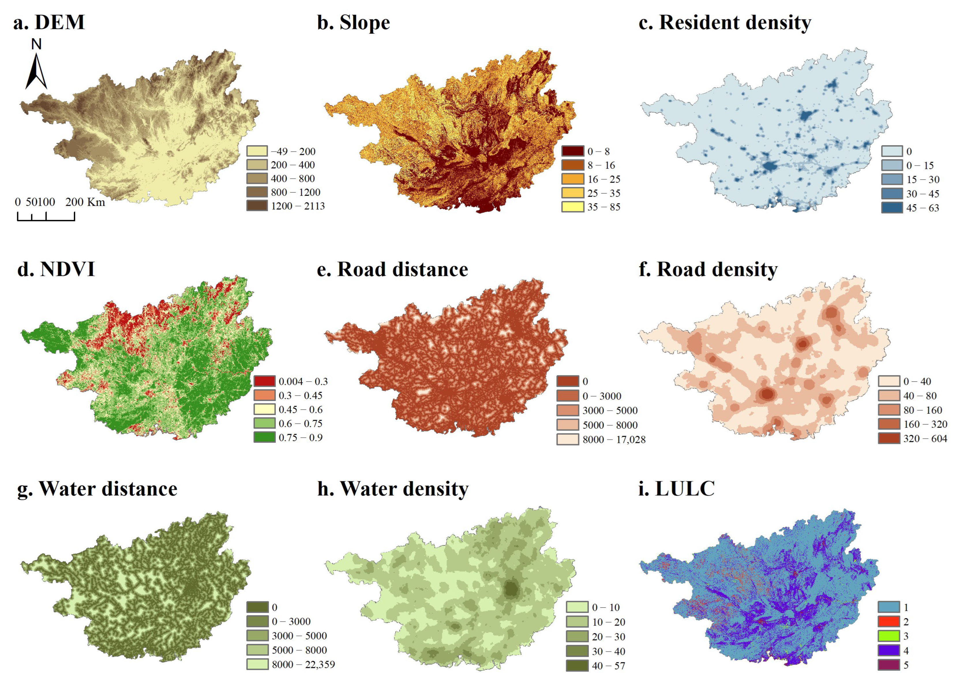
3.1.2. Resistance Surface Construction

We chose nine resistance factors from two categories—natural factors and human interference factors—based on the ecological environment in Guangxi, including elevation, slope, land-use/land-cover (LULC), distance to road, distance to water, residential density, road density, water density, and normalized difference vegetation index (NDVI). A multifactor comprehensive decision-making method is adopted to construct the resistance index system (Table 2).
Spatial principal component analysis (SPCA) is a combination of statistical theory and spatial GIS [38], and it is often used to evaluate ecological vulnerability, soil erosion, and the coupling relationship between ecology and economy. In our research, SPCA is used to transform the pixel values of nine resistance factors relative to the new axis, that is, a set of spatial variables of raster data are assigned to the correlation matrix. The final covariance and correlation matrix, eigenvalues and eigenvectors, and the percentage variance and cumulative contribution rate captured by each principal component are obtained. The natural discontinuity method is used to reclassify the raster data for each resistance factor (Table 2, Figure 3). The resistance components are weighted and added to create the final cumulative resistance surface based on the weight of each item, as determined by the spatial weight matrix. Among them, the resistance value of each pixel (the higher the value, the greater the resistance to movement) indicates the degree to which resistance factors promote or hinder movement, reflecting the cost, difficulty, or death risk of the ecological process passing through the pixel [39].

3.1.3. Identification of Ecological Corridor

The ecological corridor is usually a narrow surface area with a different appearance from the environment on both sides, formed by the linear distribution of environmental resources in space [40,41]. Generally, the ecological corridor is a relatively flat route with small obstacles, which provides a linear basis for the ecological flow to move between patches in different ecological source areas. The minimum cumulative resistance model (MCR model), which bases its calculations on the characteristics of patches, distance, and cumulative resistance, may determine how much it costs per raster unit to provide connectivity between patches. By identifying the core patches and moving resistance raster, the least-cost-path (LCP) between core patches is drawn, and then the potential possibility and trend of moving between patches, the possibility of expansion, and patch connectivity are judged [42]. The MCR model calculation formula is
R = f j = n i = m D i j × R i ,
R stands for the minimum cumulative resistance value. f is a positive correlation function between the minimum cumulative resistance and the ecological process. D i j is the distance between any raster unit i and any ecological source j .   R i the raster unit i ’s resistance to the flow of the ecological process.

3.2. Optimization of Ecological Network

Circuit theory is a concept and tool that can be applied to ecosystem research. It draws lessons from the ideas and methods of physics. Circuit theory regards an ecosystem as a network of interconnected and interactive components (such as species, communities, environment, etc.). Similar to the current flow in the circuit, there is the flow of matter and energy in the ecosystem, which is accomplished through the interaction between organisms and the environment. Components in the circuit, such as resistance, capacitance and inductance, will affect the characteristics of the circuit, and in the ecosystem, different components and interactions will also affect the structure and function of the ecosystem. For example, the competition between species and the formation of the food chain and food web can be compared to the resistance and current in the circuit. The application of circuit theory can help us to better understand and predict the changes in stability, species diversity and ecological processes in ecosystems. In addition, circuit theory can also be used to analyze and simulate ecosystems in complex networks to reveal key driving factors and interaction patterns.
Selecting patches in the proper locations to serve as the linking points of ecological sources and the priority regions for conservation and restoration is vital to maintain the complexity and stability of the network developed with a high GEP value. Ecological source patches are represented as conductive surfaces, low resistance is assigned to areas that are most permeable to movement or can promote circuit flow, and high resistance is assigned to movement obstacles [43]. The effective resistance, current, and voltage calculated across patches are related to ecological processes [44]. Circuit theory can simulate connectivity in a heterogeneous landscape environment and identify important areas to protect connectivity by reading the connected node network and resistance raster (Figure 4).
The ecological barrier is an area with a high resistance value, and there are many human interference factors. If the area can provide opportunities for ecological construction and restoration of ecological barriers, and reduce regional resistance, it will have a significant impact on the overall improvement of performance. According to circuit theory, the maximum method is adopted to detect the ecological barriers with a step length of 2500 m and a maximum search radius of 5000 m; this strategy is used to promote species migration, diffusion, or spread by introducing appropriate habitats or connections at key locations. Such spatial locations are called ecological pinch points. The principle of the research method is to generate an ecological pinch by mixing the minimum cost path generation and circuit theory to constrain the current to the optimal corridor [45,46]. The intersection of networks is the intersection of corridors with extremely low resistance; it plays a key role in enhancing the energy flow and information transmission of networks and in strengthening and consolidating the agglomeration of networks. Through artificial interference with the intersection, it is used as a supplementary stepping stone to make up for the eliminated ecological source that does not meet the area requirements but has a low resistance value. By identifying ecological barriers, ecological pinch points and supplementary stepping stones, the spatial position of the damaged or blocked ecological corridor is determined as the priority restoration area.

3.3. Analysis of Complex Networks

3.3.1. Analysis of Network Topological Attributes

In the ecological network, we take patches as points and corridors as edges to analyze the network structure and the overall performance of the network [10]. According to the topological relationship (connectivity between nodes and edges), the space and attributes of network elements are analyzed based on mathematical theoretical models. The statistical geometric quantities of network topology include average degree, clustering coefficient, eigenvector centrality, betweenness centrality, kernel number, connectivity, etc. (Table 3).

3.3.2. Calculation of Connectivity within Modules ( Z i ) and Connectivity between Modules ( P i )

Z i   and P i   are important indexes in complex network analysis, which can identify the key nodes in the pivotal position in maintaining network stability. Z i   refers to the connection strength or degree of interaction between nodes in the same module. High intra-module connectivity means that there are dense connections and close communication between nodes in the module, while low intra-module connectivity means that nodes in the module are more independent of each other. P i refers to the connection strength or degree of interaction between different modules in the network. High connectivity between modules means that there is strong connection and communication between different modules, while low connectivity between modules means that there is strong isolation between modules. Based on the degree and module division of each node in the network, according to the topological characteristics of nodes, the node attributes are divided into three types: module hubs (nodes with high connectivity within a module), connectors (nodes with high connectivity between two modules), and network hubs (nodes with high connectivity in the whole network). The above nodes play an important role in maintaining the stability of the network, and if they are missing, the network may collapse. The edges connected between key nodes are important corridors. The calculation method is as follows:
Z i = K i K S i σ K S i σ K S i
P i = 1 S = 1 N M K i s k i 2
K i is the number of edges between node i and other nodes in the module S i , K S i is the average value of   K   of all nodes in the module S i ( K is the number of connections between this node and other nodes in the module S i ), and σ K S i is the standard deviation of K values of all nodes in the module S i . K i s is the numbers of edges between node i   and nodes in module S , k i is the degree of node i , M stands for the module, and N M stands for all modules. According to the Z i   and P i   values of all nodes and their intervals, the optimal threshold is divided by combining the natural discontinuity method: module hubs, Z i > 1.34 and P i < 0.52; connectors, Z i < 1.34 and P i > 0.52; network hubs, Z i > 1.34 and P i > 0.52.

3.3.3. Network Robustness Evaluation

The structure and function of the network are mainly connection robustness and restoration robustness. Edge restoration robustness and node restoration robustness are both parts of the restoration robustness [47]. When a network changes structure, such as some nodes or edges in the network are removed or attacked (when the ecosystem is under the pressure of species extinction, environmental change, or human interference), the structure and function are maintained (the ecosystem remains stable) as connection robustness [48]. In addition, the network still has the restoration characteristics of its original nodes and corridors, referred to as restoration robustness [49,50,51].
C R = e N N r
C R is the connection robustness. e stands for the number of nodes remaining in the network’s most densely linked subgraph after some ecological nodes have been eliminated. N stands for the entire network’s node count. N r is the number of nodes eliminated.
E R = 1 M r M e M
D R = 1 N r N d N
D R is the robustness of the node that is restored. Following the removal of N r nodes, the network recovers N d nodes. E R is the robustness of edges that is restored. M r is the number of network edges that have been eliminated. M e stands for the edge’s recovery quantity. M stands for the count of edges in the network.
The robustness and resilience of the network are evaluated using random attacks and malicious attacks. Malicious attacks are intentional attacks against specific network weaknesses or key nodes. For example, destroying the living environment of key species, manipulating the food chain, or disturbing the ecological balance may lead to species extinction, energy loss, or ecological function decline. Random attacks are attacks that choose nodes in the network without purpose. They can simulate unpredictable events such as environmental change, species extinction, or other natural disasters. Through two kinds of attacks, we can help to understand the response and coping ability of ecosystems facing external interference, and then put forward corresponding protection measures.

4. Results

4.1. Ecological Network Construction

4.1.1. Initial Ecological Source

The calculated values of WCS, SCS, C/O and HP in Guangxi are USD 235.36 billion, 52.38 billion, 22.53 billion, and 34.37 billion, accounting for 68.3%, 15.2%, 6.5% and 10.9% respectively. We use the average value of each service as the standard to avoid self-influence and the mutual influence of the four ecosystem services on the ecological source selection, balance the importance of each service in the ecosystem, and choose the source with the most crucial ecosystem functions and ecological value. The first two services (WCS, SCS) select patches whose service value exceeds 20% of the average value, and the last two services (C/O, HP) select patches whose service value exceeds 30% of the average value. To avoid the influence of fine patches, we combined the high-value areas of the four ecosystem services, removed broken patches, and extracted patches with an area of more than 5 km2 as an ecological source [52,53] (Figure 5).
Four high values of ecosystem services are shown in the GEP calculation results to demonstrate geographical heterogeneity. The high values of several ecosystem services were retrieved using the average value method. According to the results, the high values of GEP are mainly concentrated in the northeast and southwest mountainous areas of Guangxi and scattered in northwest Guangxi. Low values of GEP are mainly located along the coast. We identified 456 ecological sources with a total area of 51,860.55 km2, which represents 21.82% of the entire area of Guangxi (Figure 6b). According to the land use composition of the ecological source, the ecological source is dominated by forests, which represent 94.91% of the ecological sources area and 49,052.03 km2 of the forest. In the ecological source region, the percentage of different land use types is as follows: forest > cropland > grassland > water > shrub > construction land (Table 4).

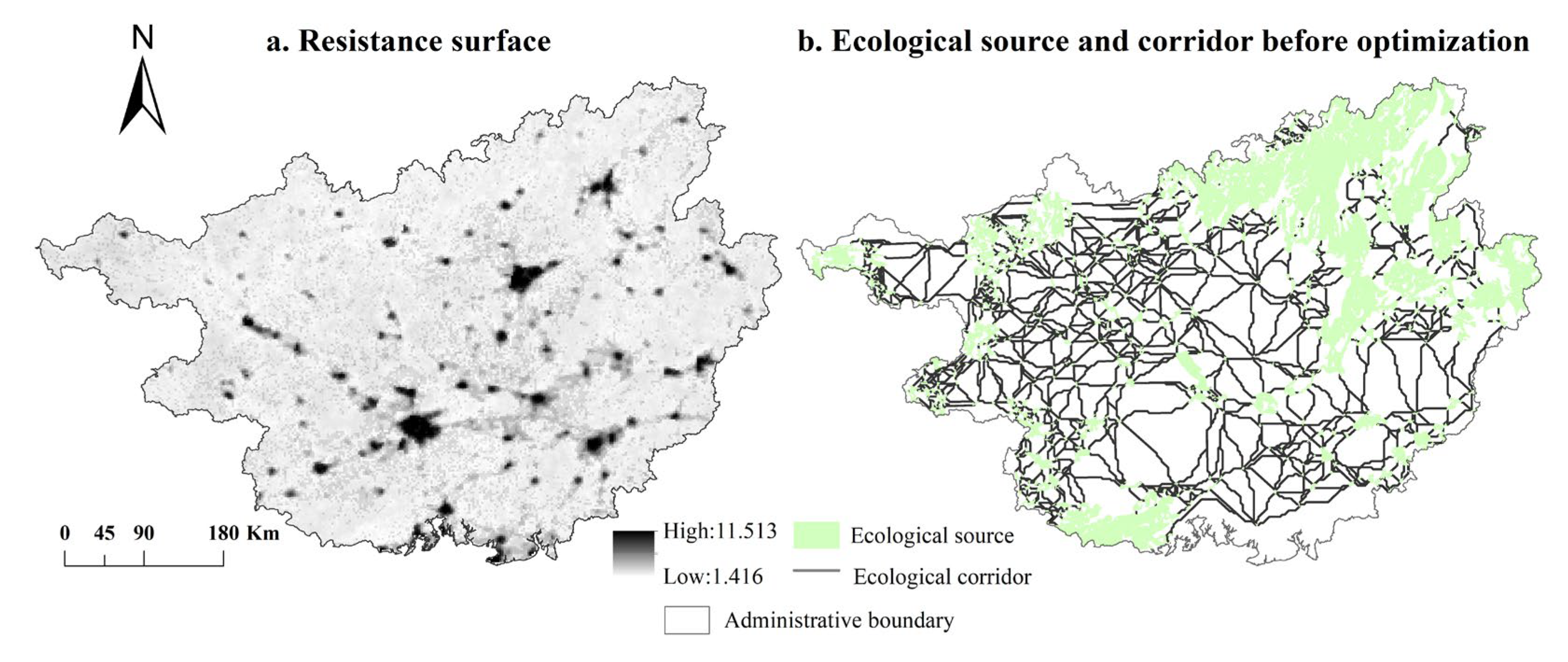
4.1.2. Construction of Resistance Surface

The results of the spatial principal component analysis of resistance factors based on natural and human interference data in Guangxi show that LULC, road distance, and population density are the most influential factors, making up 32.05%, 14.60% and 13.72% respectively. This shows that ecological resistance is mainly affected by human disturbances. Using a weighted summation of the resistance factors, a minimum cumulative resistance surface with resistance values ranging from 1.416 to 11.513 was constructed. The average ecological resistance in the entire region is 2.74. Generally speaking, the cumulative ecological resistance value decreases from city to country, and high resistance values are mainly distributed throughout urban areas (Figure 6a).

4.1.3. Initial Ecological Corridor

We extracted 1219 ecological corridors with an average length of 19.43 m (ranging from 2.29 m to 135.47 m) and a total length of 23,685.86 km based on the results of the ecological source and minimum cumulative resistance. In the entire area, ecological corridors are distributed spatially in a very distinct way, mainly concentrated in the northwest of Guangxi and parts of the south central region, with low resistance values (Figure 6b).

4.2. Enhancement and Optimization of the Ecological Network

4.2.1. Optimization Strategy

By identifying the specific spatial location, the internal defects of the ecological network are judged, and the priority areas for restoration are clearly defined. Based on the circuit theory, the ecological network is optimized. A total of 168 ecological barriers were identified, covering an area of 16,129.96 km2, and we found that large areas of barriers are mainly located in central Guangxi. Some 83 ecological pinch points were found, largely located along the administrative boundary and in the western portion of the research region, encompassing an area of 5605.52 km2. By calculating the intersection points of corridors, 71 additional stepping stones with an area of 354.52 km2 were obtained (Figure 7a). There are 778 ecological sources in the optimized ecological spatial network, 322 more than the original ecological source areas. The optimized ecological sources are 73,950.56 km2, 22,090 km2 more than the unoptimized ecological source. Finally, we extracted 2078 optimized ecological corridors with a total length of 23,922.07 km, and the total number of corridors increased by 859. After optimization, the number of ecological corridors increased in Guangxi’s central and southeast areas, and the coastal areas were directly connected to the corridors. The distribution of the ecological spatial network became more balanced, the complexity of the distribution was significantly improved, and the overall network became more dense (Figure 7b).

4.2.2. Comparison of GEP before and after Optimization

Comparing the results of GEP before and after optimization (Table 5), the GEP of the unoptimized ecological source is USD 144.50 billion, accounting for 41.93% of the GEP in Guangxi, and the GEP value of the optimized ecological source is USD 163.78 billion, accounting for 47.52% of the whole region. The newly added source areas are accompanied by a GEP of USD 19.27 billion, an increase of 13.34%. This demonstrates that by improving the ecological spatial network, the GEP of the ecological source can be improved in addition to the network’s stability and connectedness. The value offered by water conservation services before and after optimization is the highest when compared to the value of various ecosystem services in the source area, with USD 99.05 billion before optimization and USD 112.03 billion after optimization; the contribution ratio before and after optimization reached 68%. The incidental value of water conservation continues to be the largest among the values of newly added ecosystem services from source areas, increasing by USD 12.98 billion.

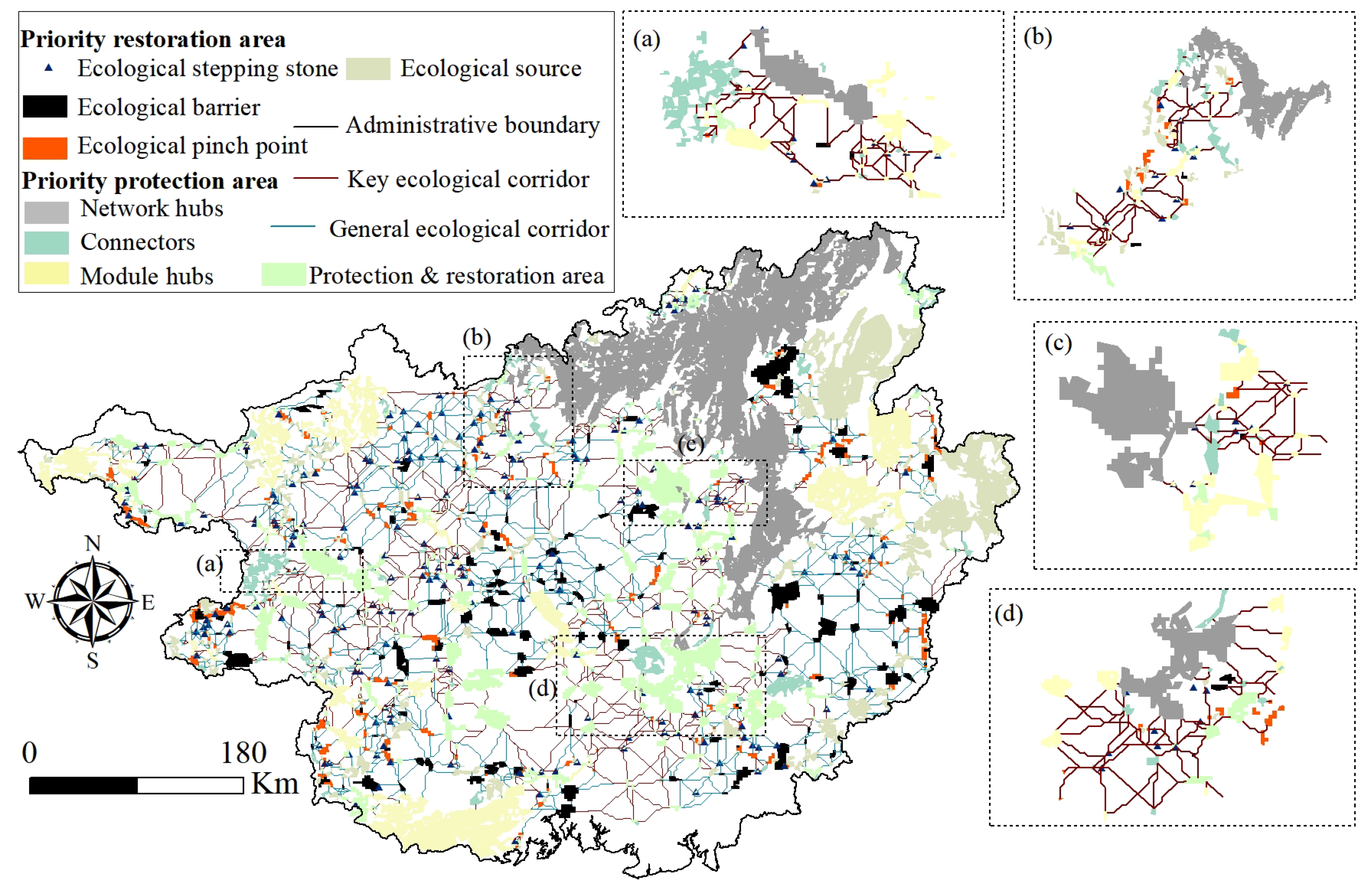
4.3. Priority Areas for Protection and Restoration

4.3.1. Module Connectivity Calculation

Connectors, module hubs, and network hubs are three types of nodes with high connectivity as priority protection areas; they ensure the connectivity of the network in the optimal range. It can be seen from Figure 8 that in the analysis of Z i and P i , the distribution of nodes in the optimized ecological network is obviously different from that before optimization. The number of nodes with high connectivity in the optimized ecological network has increased. The number of connectors has increased from 197 to 285; the number of module hubs increased from 26 to 56; and the number of network hubs has also increased from 2 to 4. We can determine the optimized three types of nodes as priority protection areas, and these areas have a total of USD 118 billion GEP (Table 6), accounting for 72% of the value of GEP attached to the optimized ecological source. In particular, the network hubs have the highest incidental value, with a GEP of USD 69.62 billion, which represents the key nature of the network center in the whole ecological network.

4.3.2. Priority Areas for Protection and Restoration

The patches corresponding to the priority areas for protection are mainly distributed in the northeast of Guangxi with high WCS, SCS, and HP values, and in the southwest of Guangxi with high C/O and HP values, with a total area of 50,869.97 km2. The restoration priority area is scattered with small patches, with a total area of 22,090 km2. The priority areas that need to be restored and protected are located in areas with high ecological resistance, i.e., most major urban areas, with a total area of 12,122.18 km2 (Figure 9a). Taking the ecological corridors that connect to nodes with high connectivity as key ecological corridors, 1018 key ecological corridors were identified, with a total length of 12,537.91 km, accounting for 52% of the total length of the optimized ecological corridors (Figure 9b).

4.4. Complex Network Analysis

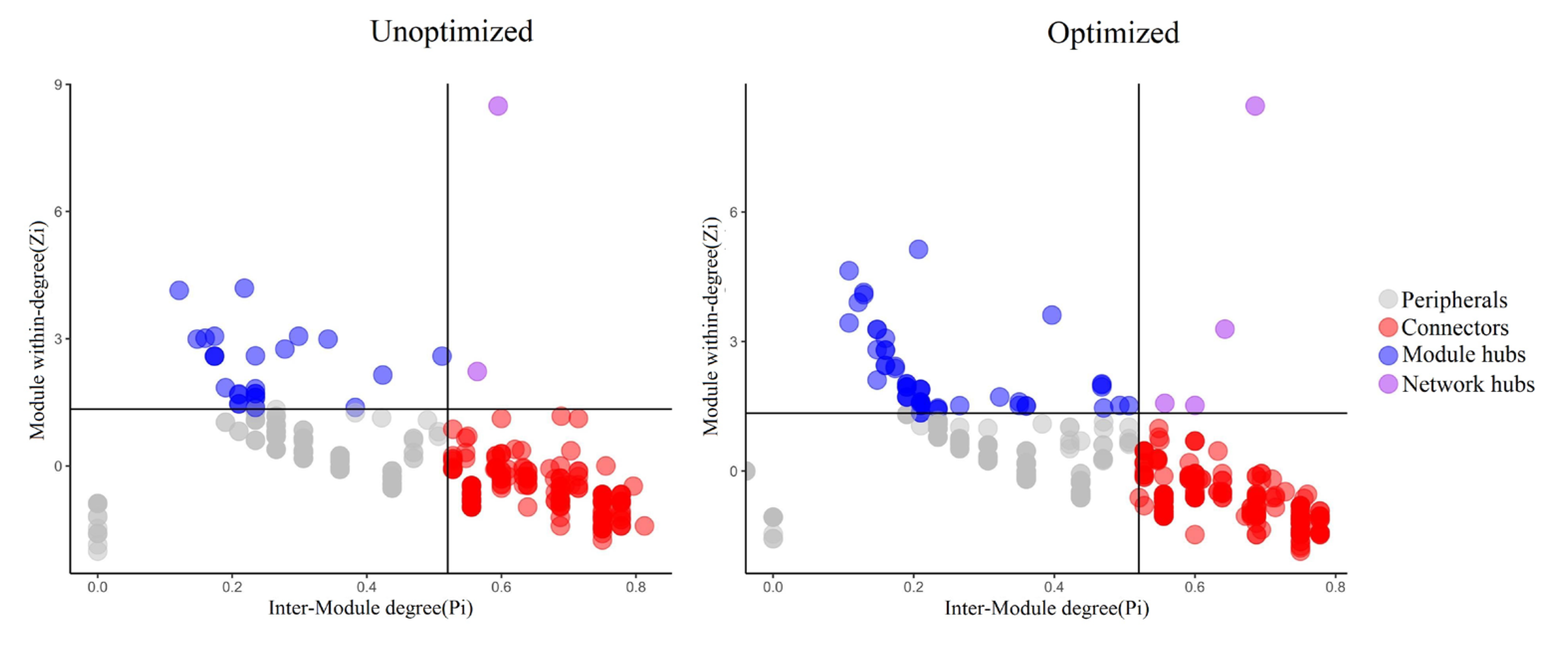
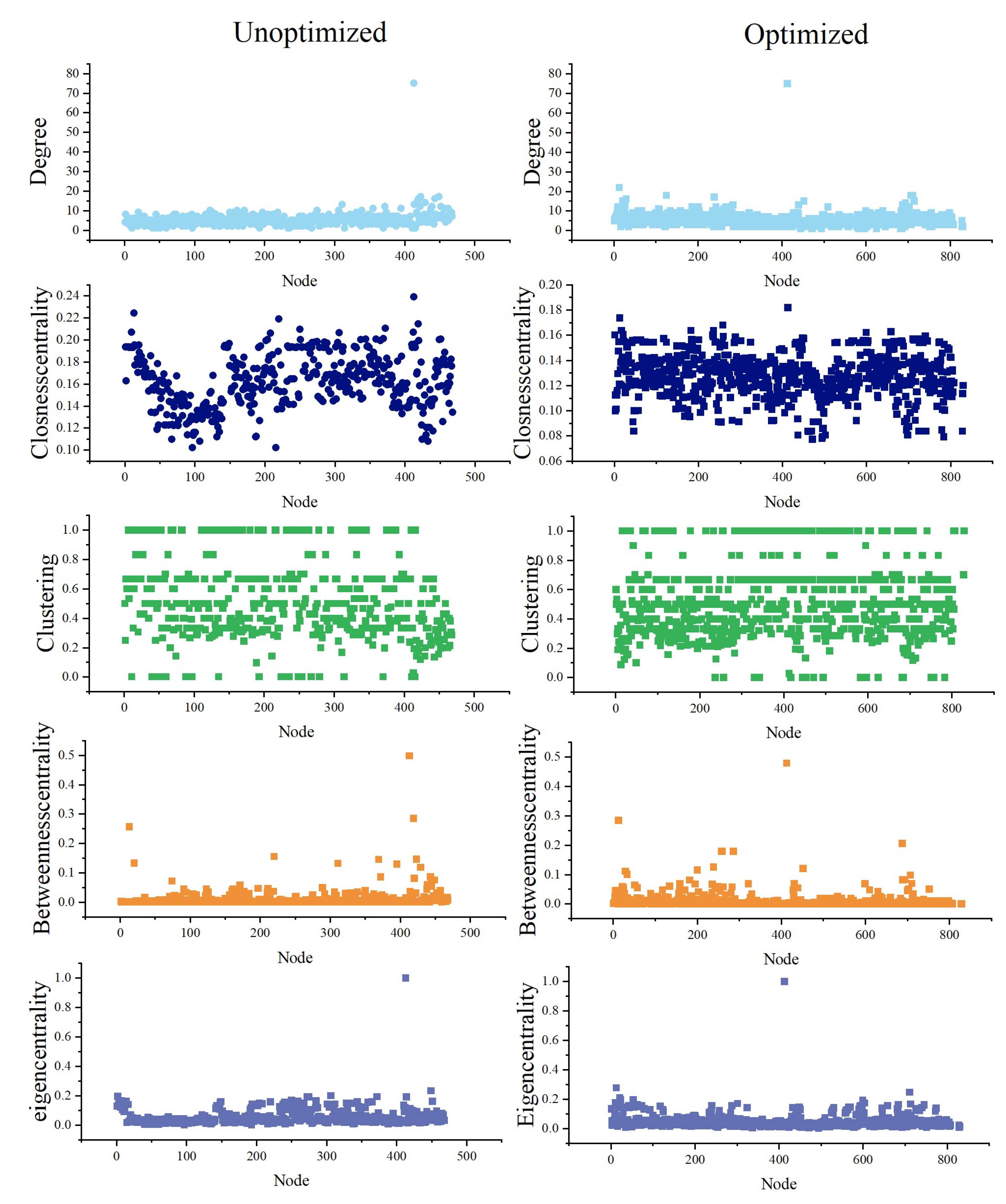
4.4.1. Analysis of Network Topology before and after Optimization

By constructing the adjacency matrix of the ecological network before and after optimization, the network properties before and after optimization are compared. After optimization, the complexity and density of the network increased significantly, and the network scale expanded. From the topology of the whole network, the average degree increased from 5.48 to 5.57, and the weighted average degree increased from 10.97 to 11.15, which improved the transmission rate and recovery rate of the optimized network. The clustering coefficient after optimization is 0.50, which is 0.004 lower than that before optimization, and the average clustering coefficient is 0.51, which is 0.01 lower than that before optimization. Generally speaking, the size of the clustering coefficient affects the propagation power of the network. When other parameters are constant, the smaller the average node clustering coefficient, the faster the propagation. The eigenvector centrality is increased from 0.04 to 0.08, and the centrality of nodes and adjacent nodes is increased, which indicates that the importance of core patches is enhanced and the connectivity between patches is improved.
Figure 10 shows the topological values of the degree and centrality of nodes. Before optimization, there were 18 nodes whose degree was greater than 10, and after optimization, there are 31 nodes whose degree is greater than 10. The degree of node 413 is the highest before and after optimization, reaching 75. There are 14 nodes with a node degree less than 2 before optimization, and 10 such nodes after optimization. The closeness centrality range of the network before optimization is from 0.23 to 0.10, and after optimization is from 0.07 to 0.18. There are 57 nodes with a network clustering of 1 before optimization, and 91 such nodes after optimization. There are three nodes with a betweenness centrality higher than 0.2 both before and after optimization; these are nodes 413, 419, and 13 (before) and nodes 413, 454, and 688 (after). The nodes with an eigenvector centrality of 1 before and after optimization are all 413. There are three nodes with eigenvector centrality less than 0.05 before optimization, and only one such node after optimization. Generally speaking, node 413 shows a high degree of concentration and transmission ability. After optimization, the importance of neighboring nodes was improved, and the performance of network nodes was significantly enhanced.

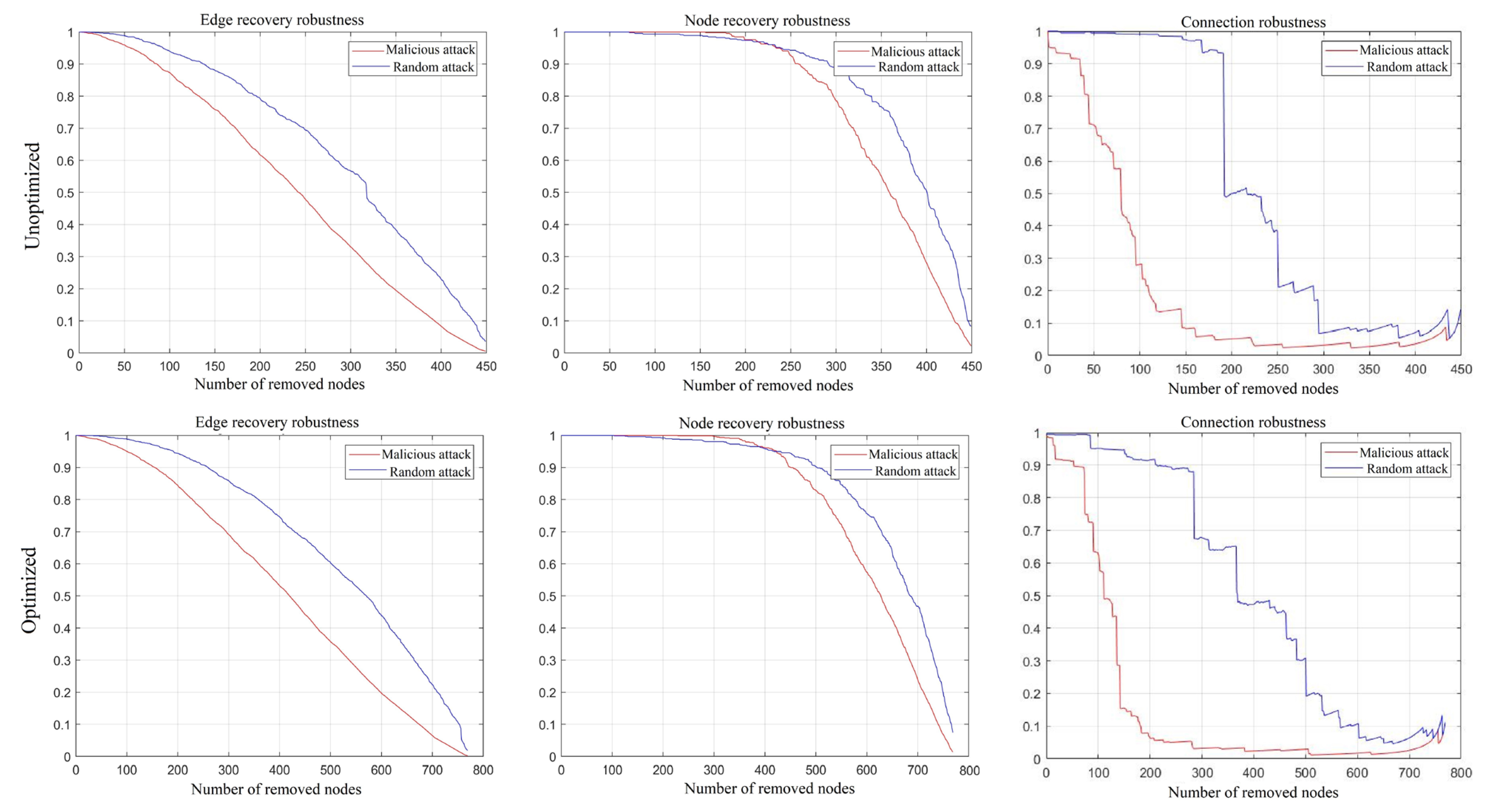
4.4.2. Comparison of Network Anti-Attack Ability before and after Optimization

By simulating random attacks and malicious attacks on ecological network nodes before and after optimization, the anti-attack ability of the network before and after optimization may be analyzed from three aspects: edge recovery robustness, node recovery robustness, and connection robustness. The initial value of network recovery robustness before and after optimization is 1. From the edge recovery robustness (Figure 11a), the performance of the optimized network is obviously improved. With the increase in the number of simulated attack nodes, the linear downward trend is smoother than that before optimization. Under malicious attacks, when the number of attack nodes in the network before the optimization is 393 (accounting for 86% of the total number of nodes), the edge recovery robustness of the optimized network is lower than 0.1 when the number of attack nodes in the network after optimization is 679 (accounting for 87% of the total number of nodes). Under random attack, when the number of attack nodes before optimization exceeds 317 (accounting for 69% of the total number of nodes), the decline speed of the optimized network is accelerated when the number of attack nodes after optimization is 618 (accounting for 79% of the total number of nodes). When the number of attack nodes before optimization is 436 (accounting for 95% of the total number of nodes), when the number of attack nodes after optimization is 754 (accounting for the 97% of the total number of nodes), the edge recovery robustness falls below 0.1, and the network nearly collapses.
From the node recovery robustness (Figure 11b), the linear decline trend in the node recovery robustness of the optimized network is smoother. The descending speed is gentler than that of the network before optimization, and there is no cliff-falling phenomenon. The robustness of node recovery decreases faster under malicious attacks than under random attacks. The node recovery robustness is higher under malicious attacks than under random attacks before the number of node attacks is less than 211 (accounting for 46% of the total number of nodes) in the network before optimization, and before the number of node attacks is less than 420 (accounting for 54% of the total number of nodes) in the network after optimization. Under malicious attacks, when the number of attack nodes in the network before the optimization is 431 (accounting for 94% of the total number of nodes), when the number of attack nodes in the optimized network is 741 (accounting for 95% of the total number of nodes), the node recovery robustness of the network is less than 0.1, and the network almost collapses. Under random attacks, when the number of node attacks in the network before optimization increases to 445 (accounting for 97% of the total number of nodes), when the number of attacks in the optimized network reaches 766 (99% of the total number of nodes), the node recovery robustness of the network is less than 0.1, and the network nearly collapses.
From the connection robustness graph, (Figure 11c), we can observe that the speed of decline in the connection robustness of the optimized network under random attacks is slower than that of the network before optimization. Under malicious attacks, the connection robustness decreases faster than under random attacks. When the number of attack nodes in the network before optimization reaches 32 (accounting for 7% of the total number of nodes), when the number of attack nodes in the optimized network reaches 73 (accounting for 9% of the total number of nodes), the connection robustness value of the network begins to decline. Under random attack, the network crashed when the number of attack nodes before optimization reached 186 (accounting for 41% of the total number of nodes), and when the number of attack nodes after optimization reached 530 (accounting for 68% of the total number of nodes). On the whole, the robustness of edge recovery, node recovery, and the connection of the optimized ecological network was improved, and the network robustness was enhanced. Among them, the robustness improvement under random attacks is more significant.

5. Discussion

5.1. Designing Biodiversity Protection Measures in Combination with an Ecological Network

To protect biodiversity, it is necessary to establish and maintain a good ecological network and ecological connectivity to promote the survival of species and the development of ecological balance. At present, research on biodiversity protection still focuses on species protection and protected land management, climate change, etc. [54,55,56]. Research on biodiversity protection combined with ecological connectivity mainly focuses on landscape indicators, species distribution models, and other methods [57]. There are few studies that combine ecology and complex networks to provide new ideas for effectively protecting biodiversity. This study provides a brand new way to understand and promote communication and migration between biological groups, which is helpful for formulating more effective protection programs and promoting the sustainable development of ecological balance.
In the design and construction of the scheme, the following issues should be considered. (1) Species difference and diversity: different species have different diffusion modes, which brings some challenges to the virtuous circle of ecosystems. Therefore, it is necessary to fully consider the differences and adaptability of different species, and to formulate corresponding management and protection measures when actually building ecological corridors and optimizing the spatial structure of ecosystems. (2) In the construction and management of ecological corridors, we may face the problem of inadvertently promoting the spread of alien invasive species. The number and diffusion range of invasive alien species can be controlled by corresponding management measures, such as vegetation selection and landscape design technology, strengthening, monitoring, and pruning. (3) Different species have different ecological requirements and diffusion patterns. For example, for species that need large-scale migration, it is necessary to set up a wide and continuous ecological corridor to ensure their movement and communication in the ecological network; for plant species living in local niches, it is necessary to strengthen the habitat protection closely related to them in order to maintain their independent living habitats. (4) Interaction between species: species competition, predation, and symbiosis affect the overall structure and function of ecological networks. In a word, biodiversity protection measures should be reasonably designed (based on optimized ecological network results) to ensure the overall health and sustainable development of the ecosystem.

5.2. Identification of Protection Priority Areas and Key Corridors

Overall, the priority area is divided into two parts; one is the priority area in the network, and the other is the priority area in the module. The ecological pinch point, ecological barrier, and stepping stone identified using circuit theory are taken as the priority recovery areas. In addition, the module hubs, network hubs, and connectors calculated using connectivity within modules ( Z i ) and connectivity between modules ( P i ) are taken as priority protection areas. If these key areas are destroyed, the whole network will become very fragile. Although important nodes in the network can be extracted by calculating the maximum value of degree, centrality, and eigenvector centrality (or by combining with the Rankpage algorithm [58,59,60,61]), these methods can not identify the more critical nodes in the network. In addition, we focus on the actual situation of the topological network, and extract the threshold value that is more in line with the data interval of this study for the calculation of Z i and P i .
In the determination of key corridors, related studies have recently tried different methods [62,63,64]. For example, five levels of corridors have been established according to centrality calculation in order to distinguish the importance of corridors. However, the classification method of corridors is fuzzy, and can not accurately identify key corridors. In this study, a new protection strategy is proposed; the most representative and critical three types of nodes and key corridors (main bridge connecting network hubs, module hubs, and connectors) in the network are identified through module connectivity calculations. This method is able to determine the important nodes and connections in the network structure in order to protect the corresponding areas and ecological corridors. Therefore, the importance of the extracted nodes and corridors is obvious; they more effectively ensure the ecological flow and balance of key areas.

5.3. Using the Insight of Protection Strategies in Future Planning

By linking the connectivity of the ecosystem with the fragmentation of key areas, and by displaying the related movement routes and areas needing protection and restoration in a comprehensive map [57,65], we can evaluate the state of the regional ecosystem more comprehensively, identify existing problems and potential threats, and take timely measures to avoid further losses and destruction, so as to ensure the sustainable and stable development of biodiversity. In addition, a comprehensive output can help planners to optimize existing planning schemes and promote the formulation of new planning schemes. At present, there are few studies on integrating various important areas and connections to assist the connectivity and planning strategy of GEP.
We have overlapped the optimized result elements and highlighted the key corridors closely connected with the network center and other comprehensive elements (such as patches that need to be repaired first). There are four network centers in the ecological network, three of which are priority areas that need to be protected and restored. In the case shown in Figure 12a, the network center point 237 has established an important connection relationship with its surrounding protection priority areas. In this case, it is necessary to focus on the ecological connectivity between the priority area and the central point, and the migration path of important species. In the case shown in Figure 12b, the important connection of some patches to the network center point 413 is selected. In this case, it is necessary to comprehensively consider various ecological elements such as general ecological sources, key areas and patches, and maintain key ecological corridors in ecological construction to promote biodiversity and ecological functions. In the case shown in Figure 12c, an important connection has been established between the network center point 21 and the protection priority areas on both sides. In this case, it is necessary to strengthen the construction of ecological corridors along the line to promote the connectivity of ecosystems in the region, and at the same time, it is necessary to pay attention to the cross-border coordination of ecological protection measures to achieve cross-border ecological flow. The case shown in Figure 12d is a combination of various elements, and the key corridor extends around them. In this case, it is necessary to establish an effective ecological corridor between the priority areas for protection and restoration, according to the structure and function of the ecosystem in the region, and to the ecological requirements of important species. At the same time, it is necessary to coordinate the planning and development activities of other sequences in the region to achieve a balance between ecological protection and sustainable economic and social development.

5.4. Optimization Strategy

From our comparative analysis of the network’s topological attributes, the results of our division via the modular calculation method are more accurate and clear. Nodes with better topological properties, such as node 413, correspond to the network hub of modularity calculation, and nodes 454 and 688 correspond to the module hub. In addition, the identified priority protection areas are consistent with the distribution of the highest GEP values of the four ecosystem services. This effectively verifies our proposed protection strategy.
In existing research, specifically speaking, the edge-increasing strategy proposing building an ecological corridor between ecological sources without corridors; this should be carried out in a specific way, based on the number of sources already present. Three different edge-increasing strategies exist: the strategy of prioritizing adding low-grade patches, the strategy prioritizing adding patches with the maximum degree of intermediation [66], and the point-increasing strategy (adding new ecological sources) [18,67]. The methods adopted include adding stepping stones at corridor breakpoints and using a similarity search to increase patches. The above method, especially the edge-increasing strategy, is based on the theoretical optimization of a topological network. It only points out which patches need added corridors, but the location and width of the newly added corridors are not clear. The optimization results may have practical significance for areas with good hydrothermal conditions (based on the premise of defining the location and width of the corridor), but may not be suitable for ecologically fragile areas. For example, it is not easy to maintain low-grade vegetation in areas with widely distributed karst landforms such as our study area. If we try to build corridors to enhance connectivity between source areas, we may destroy the original fragile natural background. The strategy of increasing patches based on similarity searches also faces similar problems. Therefore, in practice, it is most likely to play a role in identifying ecological barriers, ecological pinch points, and stepping stones as priority areas for restoration and protection through spatial analysis (as new patches based on natural background conditions). In this study, the areas of forest, shrub, wetland, grassland, cropland, water, and construction land have increased after considering ecological barriers, ecological pinch points, and stepping stones as new patches. If the newly added patches, such as construction land and cultivated land, can be transformed into real ecological sources through human intervention and transformation (for example, through returning farmland to forests and grasslands and through afforestation along the river), the feedback of GEP growth can be achieved.

5.5. Research on Existing Uncertainties and Problems

There are still some limitations in this study on the build and optimization of ecological networks, from the perspective of GEP, based on 1 km resolution source data; the evaluation of GEP only includes four ecosystem services, WCS, SCS, C/O and HP, which may neglect the value of ecosystem services provided by some regions or small regions that have made significant contributions to this region. By adopting four economic methods to calculate GEP, we can only represent the results of the influence of the region, market, and other aspects within the time range of the study. Due to differences in the selection of indicators and evaluation methods, the total value of GEP in this study is smaller than the results of previous studies [25]. Natural environmental elements and human disturbance factors are employed to build an ecological resistance surface, and an SPCA analysis and multifactor comprehensive decision approach are used to create a resistance surface with high spatial variability. However, there is room for improvement in this study’s selection of resistance factors, particularly concerning biological considerations, which were not explored in depth. Even though our research has certain difficulties and limits, the ecological spatial network we created in this study is quite important: It is helpful for the ecological construction of areas with high GEP values and areas to be prioritized for protection and restoration, and provides a specific reference for ecological space planning and the protection of ecological security in Guangxi.

6. Conclusions

In this study, the ecological network is constructed using the methods of ecological source and minimum cumulative resistance surface, and based on the circuit theory, the defects inside the network could be identified. The ecological network is then optimized using ecological barriers, pinch points, and stepping stones. Finally, combined with the complex network analysis method, priority areas for protection and restoration were determined, and the optimization effect was comprehensively evaluated. The results are as follows.
(1)
There are 456 original ecological sources in Guangxi, based on GEP extraction, with a total area of 51,860.55 km2, which represents 41.93% of the GEP in Guangxi. The northeast and the mountainous regions of the southwest are where the majority of the sources are found. There are 1219 ecological corridors, 168 ecological barriers, 83 ecological pinch points, and 71 stepping stones connecting patches in ecological source areas.
(2)
There are 778 ecological sources after optimization, and the attached GEP value reaches USD 163.78 billion, an increase of 13.33% compared with that before optimization. The area was increased by 22,090 km2. After optimization, there are 2078 ecological corridors with a combined length of 23,922.07 km, which improves the distribution of the corridors’ complexity and increases the network’s overall density.
(3)
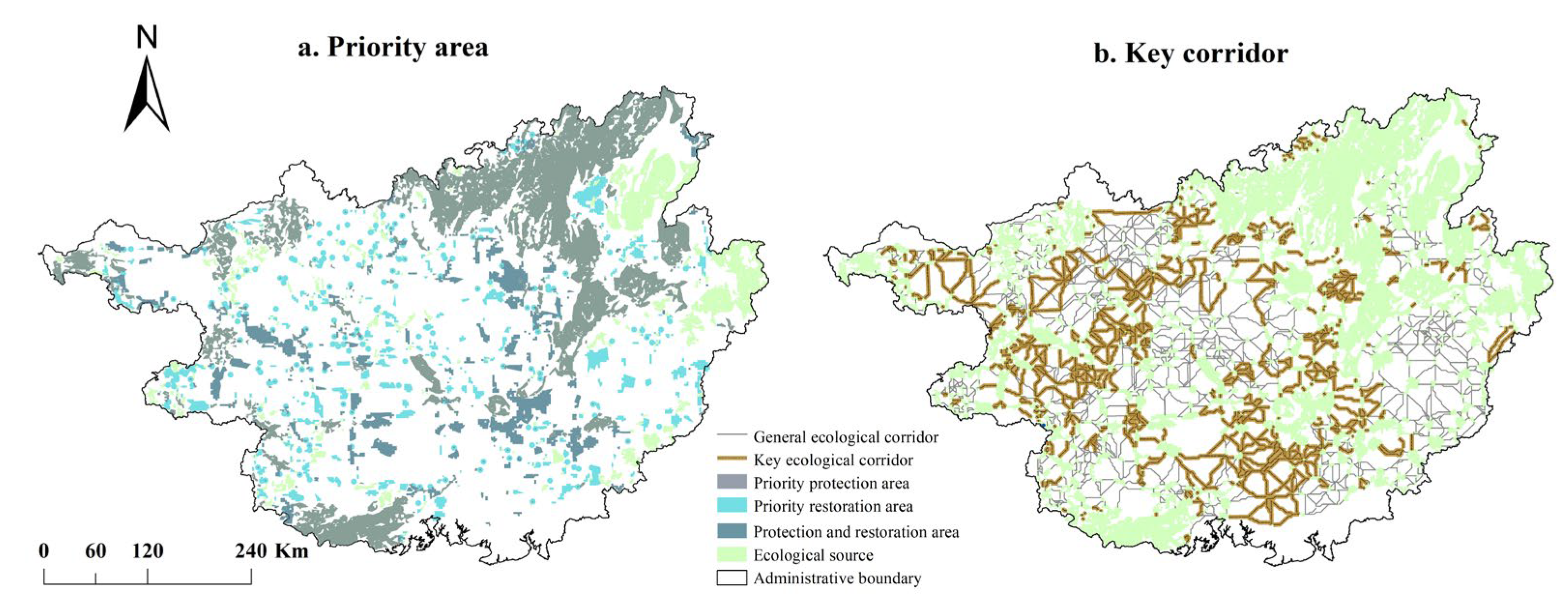
The priority areas for protection are distributed throughout a large area, with a total area of 50,869.97 km2 and a GEP of USD 118 billion. The priority areas for restoration are scattered throughout small patches, with a total area of 22,090 km2 and a GEP of USD 19.27 billion. In addition, 1018 key ecological corridors were identified, with a total length of 12,537.91 km.
(4)
Taking patches of ecological sources as nodes and corridors as edges, the complex network analysis shows that the optimized network connectivity and information transmission ability are improved, and the robustness of edge recovery, node recovery, and connection are improved. Among them, the improvement in robustness under random attack is the most remarkable.

Author Contributions

Writing—original draft preparation, L.W. and K.S.; Conceptualization, K.S., L.W. and X.J.; Writing—review & editing, K.S., X.J., J.W. and Y.Y.; Methodology, L.W. and K.S.; Data curation, L.W. and X.L.; Visualization, L.W., X.L., C.L. and S.C.; Software, K.S., L.W., C.L. and S.C.; Formal analysis, L.W., X.L. and K.S.; Supervision, S.W., X.J. and K.S.; Project administration, S.W. and X.J.; Resources, K.S. and S.W.; Funding acquisition, K.S. All authors have read and agreed to the published version of the manuscript.

Funding

This work was supported by the Open Foundation of the State Key Laboratory of Urban and Regional Ecology of China (SKLURE2023-2-3), the Youth Science Foundation of the Natural Science Foundation of Guangxi (2022GXNSFBA035570), and the Talent Introduction Program of Guangxi University (A3360051018).

Data Availability Statement

The meteorological data, soil data, land cover data are available both within this research and upon reasonable request to the authors.

Conflicts of Interest

The authors declare that they have no known competing financial interests or personal relationships that could appear to have influenced the work reported in this paper.

References

  1. Li, G.; Fang, C.; Li, Y.; Wang, Z.; Sun, S.; He, S.; Qi, W.; Bao, C.; Ma, H.; Fan, Y.; et al. Global impacts of future urban expansion on terrestrial vertebrate diversity. Nat. Commun. 2022, 13, 1628. [Google Scholar] [CrossRef] [PubMed]
  2. Lefcheck, J.S.; Byrnes, J.E.K.; Isbell, F.; Gamfeldt, L.; Griffin, J.N.; Eisenhauer, N.; Hensel, M.J.S.; Hector, A.; Cardinale, B.J.; Duffy, J.E. Biodiversity enhances ecosystem multifunctionality across trophic levels and habitats. Nat. Commun. 2015, 6, 6936. [Google Scholar] [CrossRef] [PubMed] [Green Version]
  3. Walden, E.; Queiroz, C.; Plue, J.; Lindborg, R. Biodiversity mitigates trade-offs among species functional traits underpinning multiple ecosystem services. Ecol. Lett. 2023, 26, 929–941. [Google Scholar] [CrossRef] [PubMed]
  4. Ferreira, H.M.; Magris, R.A.; Floeter, S.R.; Ferreira, C.E.L. Drivers of ecological effectiveness of marine protected areas: A meta-analytic approach from the Southwestern Atlantic Ocean (Brazil). J. Environ. Manag. 2022, 301, 113889. [Google Scholar] [CrossRef]
  5. De Souza, A.C.; Prevedello, J.A. The importance of protected areas for overexploited plants: Evidence from a biodiversity hotspot. Biol. Conserv. 2020, 243, 108482. [Google Scholar] [CrossRef]
  6. Ghosh-Harihar, M.; An, R.; Athrey, R.; Borthakur, U.; Chanchani, P.; Chetry, D.; Datta, A.; Harihar, A.; Karanth, K.K.; Mariyam, D.; et al. Protected areas and biodiversity conservation in India. Biol. Conserv. 2019, 237, 114–124. [Google Scholar] [CrossRef]
  7. Ma, T.; Lu, C.; Lei, G. The spatial overlapping analysis for Chinas natural protected area and countermeasures for the optimization and integration of protected area system. Biodivers. Sci. 2019, 27, 758–771. [Google Scholar]
  8. Puri, M.; Srivathsa, A.; Karanth, K.K.; Patel, I.; Kumar, N.S. Links in a sink: Interplay between habitat structure, ecological constraints and interactions with humans can influence connectivity conservation for tigers in forest corridors. Sci. Total Environ. 2022, 809, 151106. [Google Scholar] [CrossRef]
  9. Diniz, M.F.; Coelho, M.T.P.; Sánchez-Cuervo, A.M.; Loyola, R. How 30 years of land-use changes have affected habitat suitability and connectivity for Atlantic Forest species. Biol. Conserv. 2022, 274, 109737. [Google Scholar] [CrossRef]
  10. Pearson, R.G.; Connolly, N.M.; Davis, A.M.; Brodie, J.E. Fresh waters and estuaries of the Great Barrier Reef catchment: Effects and management of anthropogenic disturbance on biodiversity, ecology and connectivity. Mar. Pollut. Bull. 2021, 166, 112194. [Google Scholar] [CrossRef]
  11. Cunha, N.S.; Magalhaes, M.R. Methodology for mapping the national ecological network to mainland Portugal: A planning tool towards a green infrastructure. Ecol. Indic. 2019, 104, 802–818. [Google Scholar] [CrossRef]
  12. Lu, Y.; Liu, Y.; Xing, L.; Liu, Y. Robustness test of multiple protection strategies for ecological networks from the perspective of complex networks: Evidence from Wuhan Metropolitan Area, China. Land Degrad. Dev. 2023, 34, 52–71. [Google Scholar] [CrossRef]
  13. Chen, D.; Lan, Z.; Li, W. Construction of Land Ecological Security in Guangdong Province From the Perspective of Ecological Demand. J. Ecol. Rural Environ. 2019, 35, 826–835. [Google Scholar]
  14. Huang, X.; Cao, X.; Zhang, M.; Zou, X. Construction of Landscape Ecological Security Pattern of Shengli Coalfield in Inner Mongolia Based on the Minimum Cumulative Resistance Model. J. Ecol. Rural Environ. 2019, 35, 55–62. [Google Scholar]
  15. Tong, H.L.; Shi, P.J. Using ecosystem service supply and ecosystem sensitivity to identify landscape ecology security patterns in the Lanzhou-Xining urban agglomeration, China. J. Mt. Sci. 2020, 17, 2758–2773. [Google Scholar] [CrossRef]
  16. Chen, N.N.; Kang, S.Z.; Zhao, Y.H.; Zhou, Y.J.; Yan, J.; Lu, Y.R. Construction of ecological network in Qinling Mountains of Shaanxi, China based on MSPA and MCR model. Ying Yong Sheng Tai Xue Bao J. Appl. Ecol. 2021, 32, 1545–1553. [Google Scholar] [CrossRef]
  17. Cui, L.; Wang, J.; Sun, L.; Lv, C. Construction and optimization of green space ecological networks in urban fringe areas: A case study with the urban fringe area of Tongzhou district in Beijing. J. Clean. Prod. 2020, 276, 124266. [Google Scholar] [CrossRef]
  18. Zhao, S.M.; Ma, Y.F.; Wang, J.L.; You, X.Y. Landscape pattern analysis and ecological network planning of Tianjin City. Urban For. Urban Green. 2019, 46, 126479. [Google Scholar] [CrossRef]
  19. Qiu, S.; Fang, M.; Yu, Q.; Niu, T.; Liu, H.; Wang, F.; Xu, C.; Ai, M.; Zhang, J. Study of spatialtemporal changes in Chinese forest eco-space and optimization strategies for enhancing carbon sequestration capacity through ecological spatial network theory. Sci. Total Environ. 2023, 859, 160035. [Google Scholar] [CrossRef]
  20. Qiu, S.; Yu, Q.; Niu, T.; Fang, M.; Guo, H.; Liu, H.; Li, S.; Zhang, J. Restoration and renewal of ecological spatial network in mining cities for the purpose of enhancing carbon Sinks: The case of Xuzhou, China. Ecol. Indic. 2022, 143, 109313. [Google Scholar] [CrossRef]
  21. Kong, F.H.; Yin, H.W. Developing green space ecological networks in Jinan City. Acta Ecol. Sin. 2008, 28, 1711–1719. [Google Scholar]
  22. Shi, N.; Han, Y.; Wang, Q.; Quan, Z.; Luo, Z.; Ge, J.; Han, R.; Xiao, N. Construction and optimization of ecological network for protected areas in Qinghai Province. Chin. J. Ecol. 2018, 37, 1910–1916. [Google Scholar]
  23. Guo, Y.; Liu, Y. Sustainable poverty alleviation and green development in China’s underdeveloped areas. J. Geogr. Sci. 2022, 32, 23–43. [Google Scholar] [CrossRef]
  24. Wu, J.; Wu, G.; Kong, X.; Luo, Y.; Zhang, X. Why should landowners in protected areas be compensated? A theoretical framework based on value capture. Land Use Policy 2020, 95, 104640. [Google Scholar] [CrossRef]
  25. Ouyang, Z.; Zhu, C.; Yang, G.; Xu, W.; Zheng, H.; Zhang, Y. Gross ecosystem product: Concept, accounting framework and case study. Acta Ecol. Sin. 2013, 33, 6747–6761. [Google Scholar] [CrossRef]
  26. Ouyang, Z.; Zheng, H.; Xiao, Y.; Polasky, S.; Liu, J.; Xu, W.; Wang, Q.; Zhang, L.; Xiao, Y.; Rao, E.; et al. Improvements in ecosystem services from investments in natural capital. Science 2016, 352, 1455–1459. [Google Scholar] [CrossRef]
  27. Ouyang, Z.; Song, C.; Zheng, H.; Polasky, S.; Xiao, Y.; Bateman, I.J.; Liu, J.; Ruckelshaus, M.; Shi, F.; Xiao, Y.; et al. Using gross ecosystem product (GEP) to value nature in decision making. Proc. Natl. Acad. Sci. USA 2020, 117, 14593–14601. [Google Scholar] [CrossRef]
  28. Li, F.; Yan, B.; Lu, G.; Li, Z.; Zhu, X. Research on the Premise of Ecological Product Value Realization Mechanism: A Case Study of Gaochun District, Nanjing. Environ. Prot. 2021, 49, 51–58. [Google Scholar] [CrossRef]
  29. Escobedo, F.J.; Giannico, V.; Jim, C.Y.; Sanesi, G.; Lafortezza, R. Urban forests, ecosystem services, green infrastructure and nature-based solutions: Nexus or evolving metaphors? Urban For. Urban Green. 2019, 37, 3–12. [Google Scholar] [CrossRef]
  30. Raum, S.; Hand, K.L.; Hall, C.; Edwards, D.M.; O’Brien, L.; Doick, K.J. Achieving impact from ecosystem assessment and valuation of urban greenspace: The case of i-Tree Eco in Great Britain. Landsc. Urban Plan. 2019, 190, 103590. [Google Scholar] [CrossRef]
  31. Gao, M.; Hu, Y.; Bai, Y. Construction of ecological security pattern in national land space from the perspective of the community of life in mountain, water, forest, field, lake and grass: A case study in Guangxi Hechi, China—ScienceDirect. Ecol. Indic. 2022, 139, 108867. [Google Scholar] [CrossRef]
  32. Yang, Y.; Chen, J.; Lan, Y.; Zhou, G.; You, H.; Han, X.; Wang, Y.; Shi, X. Landscape Pattern and Ecological Risk Assessment in Guangxi Based on Land Use Change. Int. J. Environ. Res. Public Health 2022, 19, 1595. [Google Scholar] [CrossRef]
  33. Guangxi. Guangxi Statistical Yearbook; China Statistics Press: Beijing, China, 2021. [Google Scholar]
  34. Wang, L.; Su, K.; Jiang, X.; Zhou, X.; Yu, Z.; Chen, Z.; Wei, C.; Zhang, Y.; Liao, Z. Measuring Gross Ecosystem Product (GEP) in Guangxi, China, from 2005 to 2020. Land 2022, 11, 1213. [Google Scholar] [CrossRef]
  35. Su, K.; Liu, H.; Wang, H. Spatial-Temporal Changes and Driving Force Analysis of Ecosystems in the Loess Plateau Ecological Screen. Forests 2022, 13, 54. [Google Scholar] [CrossRef]
  36. Su, K.; Sun, X.; Guo, H.; Long, Q.; Li, S.; Mao, X.; Niu, T.; Yu, Q.; Wang, Y.; Yue, D. The establishment of a cross-regional differentiated ecological compensation scheme based on the benefit areas and benefit levels of sand-stabilization ecosystem service. J. Clean. Prod. 2020, 270, 122490. [Google Scholar] [CrossRef]
  37. Su, K.; Sun, X.; Wang, Y.; Chen, L.; Yue, D. Spatial and temporal variations of ecosystem patterns in Northern sand control barrier belt based on GIS and RS. Trans. Chin. Soc. Agric. Mach 2020, 51, 226–236. [Google Scholar]
  38. Li, Z.; Ding, Y.; Wang, Y.; Chen, J.; Fengmin, W. Construction of Ecological Security Pattern in Mountain Rocky Desertification Area Based on MCR Model: A Case Study of Nanchuan, Chongqing. J. Ecol. Rural Environ. 2020, 36, 1046–1054. [Google Scholar] [CrossRef]
  39. Li, H.H.; Ma, T.H.; Wang, K.; Tan, M.; Qu, J.F. Construction of Ecological Security Pattern in Northern Peixian Based on MCR and SPCA. J. Ecol. Rural Environ. 2020, 36, 1036–1045. [Google Scholar] [CrossRef]
  40. An, Y.; Liu, S.; Sun, Y.; Shi, F.; Beazley, R. Construction and optimization of an ecological network based on morphological spatial pattern analysis and circuit theory. Landsc. Ecol. 2021, 36, 2059–2076. [Google Scholar] [CrossRef]
  41. Liu, W.; Hughes, A.C.; Bai, Y.; Li, Z.; Mei, C.; Ma, Y. Using landscape connectivity tools to identify conservation priorities in forested areas and potential restoration priorities in rubber plantation in Xishuangbanna, Southwest China. Landsc. Ecol. 2020, 35, 389–402. [Google Scholar] [CrossRef]
  42. Su, K.; Yu, Q.; Yue, D.; Zhang, Q.; Yang, L.; Liu, Z.; Niu, T.; Sun, X. Simulation of a forest-grass ecological network in a typical desert oasis based on multiple scenes. Ecol. Model. 2019, 413, 108834. [Google Scholar] [CrossRef]
  43. Xiao, S.; Wu, W.; Guo, J.; Ou, M.; Pueppke, S.G.; Ou, W.; Tao, Y. An evaluation framework for designing ecological security patterns and prioritizing ecological corridors: Application in Jiangsu Province, China. Landsc. Ecol. 2020, 35, 2517–2534. [Google Scholar] [CrossRef]
  44. Peng, J.; Yang, Y.; Liu, Y.; Du, Y.; Meersmans, J.; Qiu, S. Linking ecosystem services and circuit theory to identify ecological security patterns. Sci. Total Environ. 2018, 644, 781–790. [Google Scholar] [CrossRef] [PubMed] [Green Version]
  45. Huang, J.; Hu, Y.; Zheng, F. Research on recognition and protection of ecological security patterns based on circuit theory: A case study of Jinan City. Environ. Sci. Pollut. Res. 2020, 27, 12414–12427. [Google Scholar] [CrossRef]
  46. Huang, L.Y.; Liu, S.H.; Fang, Y.; Zou, L. Construction of Wuhan’s ecological security pattern under the “quality-risk-requirement” framework. J. Appl. Ecol. 2019, 30, 615–626. [Google Scholar] [CrossRef]
  47. Guo, H.; Yu, Q.; Pei, Y.; Wang, G.; Yue, D. Optimization of landscape spatial structure aiming at achieving carbon neutrality in desert and mining areas. J. Clean. Prod. 2021, 322, 129156. [Google Scholar] [CrossRef]
  48. Peng, G.; Wu, J. Optimal network topology for structural robustness based on natural connectivity. Phys. A Stat. Mech. Its Appl. 2016, 443, 212–220. [Google Scholar] [CrossRef]
  49. Murray, A.T.; Church, R.L.; Pludow, B.A. Enhanced solution capabilities for multiple patch land allocation. Comput. Environ. Urban Syst. 2022, 97, 101871. [Google Scholar] [CrossRef]
  50. Shen, Z.; Wu, W.; Chen, S.; Tian, S.; Wang, J.; Li, L. A static and dynamic coupling approach for maintaining ecological networks connectivity in rapid urbanization contexts. J. Clean. Prod. 2022, 369, 133375. [Google Scholar] [CrossRef]
  51. Qiu, S.; Yu, Q.; Niu, T.; Fang, M.; Guo, H.; Liu, H.; Li, S. Study on the Landscape Space of Typical Mining Areas in Xuzhou City from 2000 to 2020 and Optimization Strategies for Carbon Sink Enhancement. Remote Sens. 2022, 14, 4185. [Google Scholar] [CrossRef]
  52. Wu, J.; Zhang, S.; Luo, Y.; Wang, H.; Zhao, Y. Assessment of risks to habitat connectivity through the stepping-stone theory: A case study from Shenzhen, China. Urban For. Urban Green. 2022, 71, 127532. [Google Scholar] [CrossRef]
  53. Zhang, Y.; Jiang, Z.; Li, Y.; Yang, Z.; Wang, X.; Li, X. Construction and optimization of an urban ecological security pattern based on habitat quality assessment and the minimum cumulative resistance model in Shenzhen city, China. Forests 2021, 12, 847. [Google Scholar] [CrossRef]
  54. Gorman, C.E.; Torsney, A.; Gaughran, A.; McKeon, C.M.; Farrell, C.A.; White, C.; Donohue, I.; Stout, J.C.; Buckley, Y.M. Reconciling climate action with the need for biodiversity protection, restoration and rehabilitation. Sci. Total Environ. 2023, 857, 159316. [Google Scholar] [CrossRef]
  55. Shipley, J.R.; Gossner, M.M.; Rigling, A.; Krumm, F. Conserving forest insect biodiversity requires the protection of key habitat features. Trends Ecol. Evol. 2023, 4, 3172. [Google Scholar] [CrossRef]
  56. Stubenrauch, J.; Garske, B. Forest protection in the EU's renewable energy directive and nature conservation legislation in light of the climate and biodiversity crisis—Identifying legal shortcomings and solutions. For. Policy Econ. 2023, 153, 102996. [Google Scholar] [CrossRef]
  57. Babí Almenar, J.; Bolowich, A.; Elliot, T.; Geneletti, D.; Sonnemann, G.; Rugani, B. Assessing habitat loss, fragmentation and ecological connectivity in Luxembourg to support spatial planning. Landsc. Urban Plan. 2019, 189, 335–351. [Google Scholar] [CrossRef]
  58. Song, S.; Xu, D.; Hu, S.; Shi, M. Ecological Network Optimization in Urban Central District Based on Complex Network Theory: A Case Study with the Urban Central District of Harbin. Int. J. Environ. Res. Public Health 2021, 18, 1427. [Google Scholar] [CrossRef]
  59. Wang, H.; Li, W.; Hou, Y.; Li, M.; Lee, S.-Y. The Construction of Urban Park Green Infrastructure Network Based on Genetic Algorithm. Wirel. Commun. Mob. Comput. 2022, 2022, 9719633. [Google Scholar] [CrossRef]
  60. Wang, R. Ecological network analysis of China’s energy-related input from the supply side. J. Clean. Prod. 2020, 272, 122796. [Google Scholar] [CrossRef]
  61. Tang, F.; Zhou, X.; Wang, L.; Zhang, Y.; Fu, M.; Zhang, P. Linking ecosystem service and MSPA to construct landscape ecological network of the Huaiyang Section of the Grand Canal. Land 2021, 10, 919. [Google Scholar] [CrossRef]
  62. Jalkanen, J.; Toivonen, T.; Moilanen, A. Identification of ecological networks for land-use planning with spatial conservation prioritization. Landsc. Ecol. 2020, 35, 353–371. [Google Scholar] [CrossRef] [Green Version]
  63. Li, L.; Huang, X.; Wu, D.; Wang, Z.; Yang, H. Optimization of ecological security patterns considering both natural and social disturbances in China's largest urban agglomeration. Ecol. Eng. 2022, 180, 106647. [Google Scholar] [CrossRef]
  64. Wang, Y.; Qu, Z.; Zhong, Q.; Zhang, Q.; Zhang, L.; Zhang, R.; Yi, Y.; Zhang, G.; Li, X.; Liu, J. Delimitation of ecological corridors in a highly urbanizing region based on circuit theory and MSPA. Ecol. Indic. 2022, 142, 109258. [Google Scholar] [CrossRef]
  65. Huang, L.; Wang, J.; Fang, Y.; Zhai, T.; Cheng, H. An integrated approach towards spatial identification of restored and conserved priority areas of ecological network for implementation planning in metropolitan region. Sustain. Cities Soc. 2021, 69, 102865. [Google Scholar] [CrossRef]
  66. Yang, L.Z.; Niu, T.; Yu, Q.; Yue, D.P.; Ma, J.; Pei, R.Y. Ecological spatial optimization based on complex network theory: A case study of Songhua River Basin. J. Beijing For. Univ. 2022, 44, 91–103. [Google Scholar]
  67. Dong, J.; Peng, J.; Liu, Y.; Qiu, S.; Han, Y. Integrating spatial continuous wavelet transform and kernel density estimation to identify ecological corridors in megacities. Landsc. Urban Plan. 2020, 199, 103815. [Google Scholar] [CrossRef]
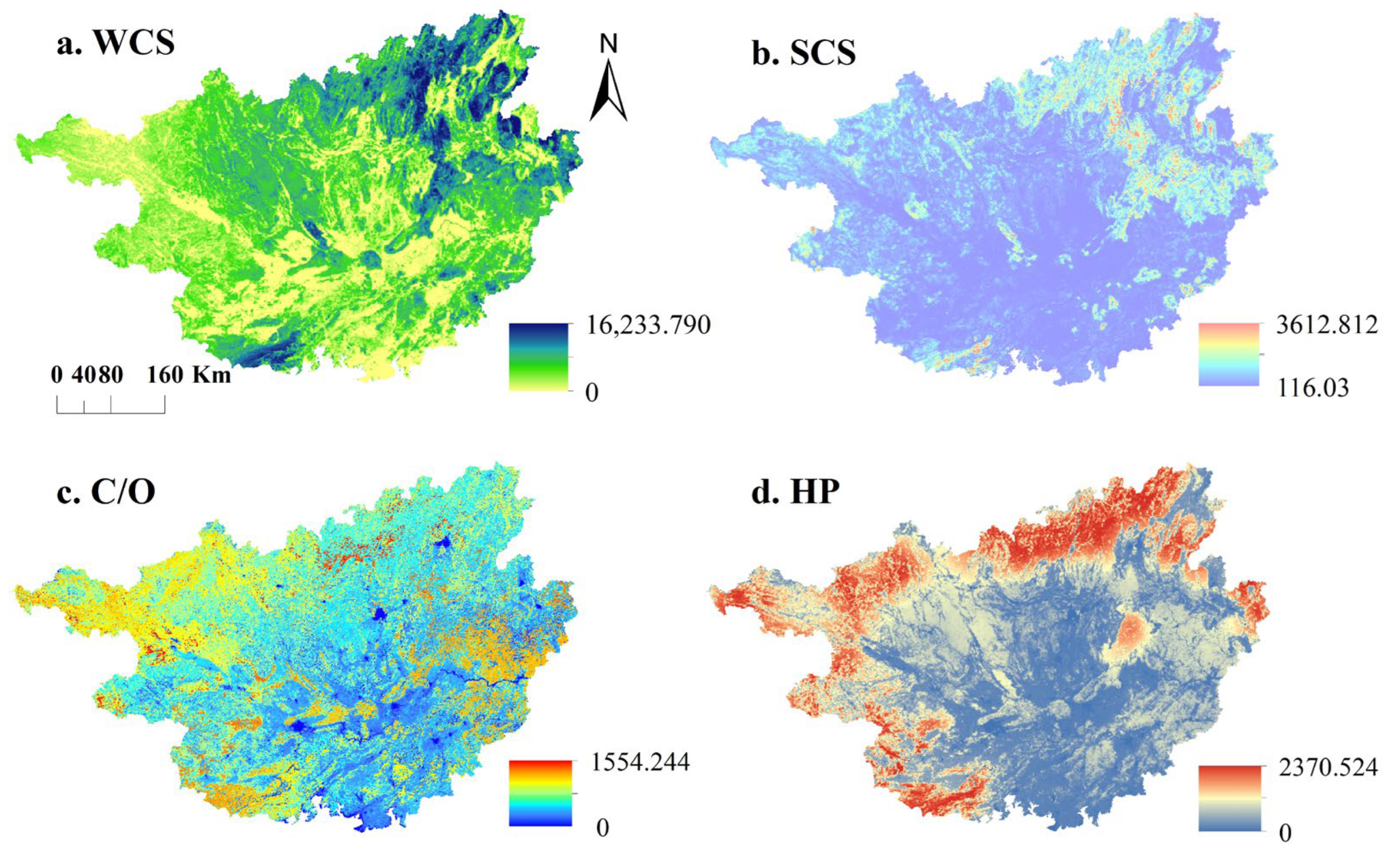
Figure 1. Location of the study area.
Remotesensing 15 03420 g001
Figure 2. Technological workflow: by quantifying various ecosystem services and their eco-economic values and determining ecological sources combined with natural conditions and human activities, the ecological resistance surface was constructed via spatial principal component analysis (SPCA). The minimum cumulative resistance model (MCR model) and loop theory are used to extract ecological corridors, ecological barriers, ecological pinch points, and ecological stepping stones to optimize the ecological space network. Finally, the performance of the ecological space network before and after optimization is compared and analyzed.
Remotesensing 15 03420 g002
Figure 3. Spatial distribution of resistance level.
Remotesensing 15 03420 g003
Figure 4. Circuit theory. The electricity raster is represented by a resistance raster, and the ecological source patches are used as nodes (represented by a dot). Adjacent patches are connected to their four or eight neighbors through resistors. The two short-circuit areas are folded into a single node, and the infinite resistance (high resistance value) unit is completely separated from the network.
Remotesensing 15 03420 g004
Figure 5. Spatial distribution of GEP.
Remotesensing 15 03420 g005
Figure 6. (a) Minimum cumulative resistance surface. (b) Initial ecological source and corridor.
Remotesensing 15 03420 g006
Figure 7. Optimized ecological spatial network.
Remotesensing 15 03420 g007
Figure 8. Calculation of connectivity within modules ( Z i ) and Connectivity between Modules ( P i ).
Remotesensing 15 03420 g008
Figure 9. Distribution of priority areas and key corridors.
Remotesensing 15 03420 g009
Figure 10. Topological properties of nodes.
Remotesensing 15 03420 g010
Figure 11. Robustness of ecological space network before and after optimization.
Remotesensing 15 03420 g011
Figure 12. Overlay mapping highlighting the network hubs. (a) Zoom of the network hub 237 and key corridors and other elements. (b) The overlay zoom diagram of the patch and key corridors and other elements of the partial area of the network hub 413. (c) Zoom of the network hub 21 and key corridors and other elements. (d) Zoom of the network hub 13 and key corridors and other elements.
Remotesensing 15 03420 g012
Table 1. Calculation of gross ecosystem product (GEP). Combined with geographical attribute data such as meteorology, topography and land use, the biophysical quantities of each index are obtained by studying their correlation; according to the local prices of water, soil, carbon, oxygen, and species conservation in Guangxi, the values of corresponding indicators are calculated to quantify the value of ecosystem services.
ItemDescribeBiophysical
Quantities
MethodValue QuantityMethodNote
Water Conservation Service (WCS) The   calculation   is   based   on   the   relationship   between   water   conservation   ( W C )   and   annual   precipitation   ( P R E ) , annual evapotranspiration ( E T )   and   annual   storm   runoff   ( Q F ). W C = P R E E T Q F Water Balance Equation C W C = S O
V W C = W C × C W C
Shadow engineering methodThe ratio of the annual fixed investment in water conservancy S in Guangxi to the reservoir construction capacity O is taken as the price C W C of the reservoir construction project.
Soil Conservation Service (SCS) Calculation   of   soil   conservation   ( S C ) of vegetation by the quantitative model of soil loss S C = S E p S E a
= R · K · L S · 1 C O G
Universal Soil Loss Equation (USLE) C S C = E R
V S C = S C × C S C
Replacement cost methodThe ratio of the investment E in comprehensive soil erosion control in the small watershed of Guangxi to the area R of the soil erosion control is taken as the price C S C   of the soil erosion control project.
Carbon Sequestration and Oxygen Release Services (C/O) According   to   the   biomass   of   each   ecosystem ,   the   carbon   sequestration   ( C O S ) and oxygen release ( C O P ) are calculated. C O S = i = 1 j A G B i × C i
C O P = M O 2 / M C O 2 × C O S
Remote sensing inversion, model simulation, and measured data V C O S = C O S × C C O S
V C O P = C O P × C C O P
V C O = V C O S + V C O P
Market price methodEconomic prices are carbon trading price C C O S and industrial oxygen price C C O P respectively.
Habitat Provision (HP)Estimation of biological distribution quantity based on habitat quality and habitat scarcity ( E ) E = i = 1 n E i Estimation of biological distribution quantity V E = E × C E Shannon–Wiener index gradeThe conservation value of species per unit area C E is taken as the price.
PS: V W C is the value of water conservation. S E p and S E a are potential soil erosion and actual soil erosion [35], respectively [t/(hm2∙a)]; R is the rainfall erosivity factor, MJ∙mm/(hm2∙h∙a); K is the soil erodibility factor, t∙hm2∙h/(hm2∙MJ∙mm); L S   and C O G are terrain factors and vegetation coverage factors, respectively, and they are dimensionless [36,37]. V S C is the value of the soil conservation service. A G B i is the aboveground biomass of the i ecosystem type; C i is the biomass–carbon conversion coefficient of the i ecosystem type; M O 2 / M C O 2 = 32 / 44 is the coefficient for the transformation of C O 2 into O 2 ; V C O S is the value of the carbon sequestration service; V C O P is the value of the oxygen release service; V C O is the total value of both the carbon sequestration and oxygen release service.
Table 2. Resistance factors and gradation of ecological source expansion.
Resistance Factor12345Weight
DEM−15–200200–400400–800800–12001200–21130.056
Slope0–88–1616–2525–3535–850.045
LULCForestGrass/shrubsWaterCroplandConstruction land0.320
Residential density00–1515–3030–4545–620.137
Road distance (m)8000–17,0005000–80003000–50000–300000.060
Water distance (m)00–30003000–50005000–80008000–22,0000.140
Road density320–600160–32080–16040–80400.146
Water density0.05–1010–2020–3030–4040–600.037
NDVI0.75–0.90.6–0.750.45–0.60.3–0.450.05–0.30.094
Table 3. Summary of topological attribute calculation methods.
Topological AttributeCalculation MethodDescribeNote
Average degree K = 1 N i = 1 N K i The relationship between the number of patches (nodes) and the number of patches (edges) K is the average degree. N is the number of patches. L is the number of patch edges.
Network diameter L m a x = m a x d i j The   maximum   value   of   the   shortest   distance   between   any   two   points   in   the   network   ( L m a x ) d i j is the shortest distance from node i to node j .
Clustering coefficient C i = 2 E i K i K i 1 The degree of interconnection between adjacent points of a point.The clustering coefficient C i is the ratio of the actual number of edges E i between K i neighboring nodes of a node to the total number of possible edges.
Eigenvector centrality X i = 1 σ k a k i X k
σ X = X A
A measure of the transmission influence and connectivity between patches.The center vector X is the left eigenvector of the adjacency matrix A associated with the eigenvalues σ . σ as the largest eigenvalue in the absolute value of the matrix A .
Betweenness centrality C B = s t N σ s t N σ s t The number of times a node acts as a bridge for the shortest path between the other two nodes. C B represents the center of the number of nodes i . σ s t N is the shortest paths from node s to node t through node N , and σ s t is the shortest path from node s to node t .
Closeness centrality C C = v 1 i v d v i Generally speaking, the distance between a transit patch and other patches is the shortest. C C is the closeness centrality of node i , and is used to calculate the number of direct connections between node i ( i v ) and other nodes. i v d v i is the sum of the cell values of the corresponding rows or columns of nodes i in the network matrix.
Table 4. The proportion of LULC in ecological sources.
LULCUnoptimizedOptimized
Area (km2)Proportion (%)Area (km2)Proportion (%)
Cropland1874.933.6310,779.8814.64
Forest49,052.0394.9160,485.2582.14
Grassland571.711.111032.551.40
Shrub34.940.0756.210.08
Water128.480.25510.700.69
Construction land22.450.04774.591.05
Table 5. GEP (billion USD) of the ecological source.
GEPWCSSCSC/OHPALL
Guangxi 235.3652.3822.5334.37344.64
Unoptimized ecological source99.0526.605.3413.51144.50
Optimized ecological source112.0328.997.2315.53163.78
Add ecological source12.982.391.892.0219.27
Table 6. Classification of nodes with high connectivity and corresponding GEP.
Modularity IndexNumber of NodesArea (Km2)WCSSCSC/OHPGEP (Billion USD)
Connectors2858482.368.651.830.851.2712.59
Module hubs5616,978.7223.876.361.773.7935.79
Network hubs425,408.8948.2212.972.436.0169.62
Disclaimer/Publisher’s Note: The statements, opinions and data contained in all publications are solely those of the individual author(s) and contributor(s) and not of MDPI and/or the editor(s). MDPI and/or the editor(s) disclaim responsibility for any injury to people or property resulting from any ideas, methods, instructions or products referred to in the content.

