Article

When Convolutional Neural Networks Meet Laser-Induced Breakdown Spectroscopy: End-to-End Quantitative Analysis Modeling of ChemCam Spectral Data for Major Elements Based on Ensemble Convolutional Neural Networks

1
Intelligent Robotics Lab, School of Artificial Intelligence, Jilin University, Changchun 130012, China
2
Engineering Research Center of Knowledge-Driven Human–Machine Intelligence, Ministry of Education, Changchun 130012, China
*
Author to whom correspondence should be addressed.
Remote Sens. 2023, 15(13), 3422; https://doi.org/10.3390/rs15133422
Submission received: 26 May 2023 / Revised: 27 June 2023 / Accepted: 5 July 2023 / Published: 6 July 2023

Abstract

:
Modeling the quantitative relationship between target components and measured spectral information is an essential part of laser-induced breakdown spectroscopy (LIBS) analysis. However, many traditional multivariate analysis algorithms must reduce the spectral dimension or extract the characteristic spectral lines in advance, which may result in information loss and reduced accuracy. Indeed, improving the precision and interpretability of LIBS quantitative analysis is a critical challenge in Mars exploration. To solve this problem, this paper proposes an end-to-end lightweight quantitative modeling framework based on ensemble convolutional neural networks (ECNNs). This method eliminates the need for dimensionality reduction of the raw spectrum along with other pre-processing operations. We used the ChemCam calibration dataset as an example to verify the effectiveness of the proposed approach. Compared with partial least squares regression (a linear method) and extreme learning machine (a nonlinear method), our proposed method resulted in a lower root-mean-square error for major element prediction (54% and 73% lower, respectively) and was more stable. We also delved into the internal learning mechanism of the deep CNN model to understand how it hierarchically extracts spectral information features. The experimental results demonstrate that the easy-to-use ECNN-based regression model achieves excellent prediction performance while maintaining interpretability.

Graphical Abstract

1. Introduction

Laser-induced breakdown spectroscopy (LIBS) is a type of atomic emission spectroscopy that uses laser pulses as the excitation source to induce the generation of laser plasma [1]. Given the unique features of surface detection on Mars, the long-range detection, efficient and fast analysis, and multifunctional sampling protocols of LIBS provide it with advantages over other spectroscopic techniques for Mars surface analysis. Therefore, LIBS has become recognized as an advanced space exploration technique with tremendous advantages [2]. The ChemCam instrument on board the Curiosity rover that landed on Mars in 2012 was the first LIBS device for planetary exploration. The ChemCam engineering model is primarily composed of three spectrometers, a remote micro-imager, a telescope, a laser, a demultiplexer, and associated digital and electronic devices. The laser source of the instrument is Nd: KGW 1067 nm, whose frequency range is 3–10 Hz, and pulsed laser energy can be up to 14 m with a 5-ns duration when the temperature is below 0 °C. The light from the generated plasma is captured through a 110 mm diameter telescope and transmitted via optical fiber to a group of three Czerny-Turner spectrometers (covering 240–850 nm) [3]. The primary purpose of Martian LIBS is to determine the chemical compositions of rocks and soil. The ChemCam team routinely reports compositions for eight major elements (Si, Al, K, Ti, Mg, Fe, Na, Ca). However, due to the LIBS technique outputting complex spectral data containing peak overlaps and interference between characteristic spectral lines, it has been a stiff challenge to analyze complex high-dimensional spectral data efficiently and accurately. In this study, the major elements Si, Al, and K were analyzed because they cover three representative ranges, and their concentration differences are important characteristic indexes that reflect the variation of sedimentary conditions [4]. They are also widely chosen as examples for mineral identification, emission line selection, element abundance identification, and other LIBS tasks [3,5,6].
LIBS multivariate quantification methods can be divided into two categories: linear and nonlinear. Multiple linear regression is a common linear analysis method. However, the collinearity of spectral variables affects the accuracy of the parameter estimation. In addition, when the available spectral data are limited, the model is prone to overfitting. Although principal component regression and partial least squares regression (PLS) models solve the collinearity problem of independent variables, they are not applicable in cases with complex nonlinear relationships between the spectral data and the variables to be collected due to spectral overlap and changes. Nonlinear modeling methods include support vector regression (SVR), decision trees, and artificial neural networks (ANNs). However, dimensionality reduction or feature extraction must be performed on the spectral data before nonlinear modeling due to the curse of dimensionality. Variable selection provides a simple option for model interpretation by removing uninformative wavelengths or choosing a subset of the most relevant wavelengths [7]. However, feature extraction and modeling are two independent processes, and the extracted features do not necessarily reflect the true mapping relationship between the spectra and the predicted values. If useful features are discarded and noise is retained during feature extraction, the results will deviate from the actual mathematical model. In that respect, traditional feature selection and modeling methods cannot fully mine the useful information in the given data and are prone to losing useful information and introducing man-made noise. Therefore, using one or a few emission lines is insufficient for acquiring comprehensive information about the plasma systems of interest. While the feature emission lines of analyte elements are the main signatures of LIBS analysis, the lines of non-analyte elements can also play an essential role [8]. A LIBS spectrum should thus be considered as an organic whole with an ordered structure rather than a scattering of isolated data points. Full-spectrum analysis can potentially overcome these limitations. Thus, it is necessary to develop a data-knowledge, dual-drive modeling method [9,10,11,12] that reduces the need for empirical knowledge and can automatically extract useful information from a spectrum to improve the model’s predictive ability, thereby reducing the threshold for LIBS modeling.
In recent years, with the development of deep learning algorithms, a new wave of artificial intelligence has arrived. A series of end-to-end deep learning algorithms represented by convolutional neural networks (CNNs) can automatically extract the intrinsic features of the data without data pre-processing (e.g., dimensionality reduction and feature selection). The entire feature extraction operation is like viewing an object from the microscopic to macroscopic scale using a microscope. Good regression analysis results were obtained for one-dimensional (1D) near-infrared data using a CNN structure [13,14,15]. The few existing LIBS-related fundamental studies using CNNs for regression problems are the milestones. Cao et al. [16] discussed using the Inception V2 network to analyze the concentration of oxides in Martian soil. The model resulted in better performance for the quantification of oxides compared to models based on PLS and SVR. Zhang et al. [17] utilized the Resnet network to quantify the elemental composition from LIBS signals on Mars, which effectively reduced the prediction error of the measured elements. Li et al. [18] developed a deep CNN-based LIBS multi-component quantitative analysis method for geological samples, which is an excellent attempt to apply the convolutional neural network to one-dimensional LIBS data and achieve good results.
The methods mentioned above have demonstrated the potential of using deep learning techniques to develop prediction models for spectral fields. Nevertheless, these existing CNN models still follow conventions of data-driven deep CNNs for designing deeper and more complex architectures. They are computationally expensive, and the authors only provided a summary of the hyperparameters, without disclosing any information as to how architecture hyperparameter selection was accomplished. The relationships between model generalizability and parameters are unclear. To address this problem, we focus on the three following topology-related parameters: stride step, number of convolutional kernels (NCK), and convolutional kernel width (CKW) [19,20]. We first investigated the effects of these parameters in detail and proposed a two-step progressive strategy to acquire the best parameters. From the above studies, we also observed that despite the designed deep CNNs having deep learning abilities, it is hard to interpret the specific “features”, which impedes its practical application exactly. Therefore, it is also worthwhile to try the approaches to interpret CNN results. In this study, we show how the CNN model works on spectral data by visualizing the feature maps in convolutional layers.
However, a single 1D CNN usually performs poorly when dealing with regression analysis problems, especially when the calibration dataset is insufficient. In this work, to further enhance the predictive ability of the CNN model, the model is optimized from the perspective of a model ensemble. Ensemble learning achieves better prediction performance by combining multiple weakly supervised models into a more comprehensive supervised model [21]. Considerable research has shown that ensemble modeling is one of the most effective solutions to reduce over-fitting [22,23] and improves the stability and accuracy of a single model. The ensemble learning methods for 1D data processing in most reported studies applied classical PLS regression models as their base estimators [24]. Popular ensemble techniques, such as stacked generalization (stacking) [25], boosting [26], and bagging [27], are then used to improve and integrate the prediction results of the basic PLS model. Zhou et al. [28] compared boosting PLS and bagging PLS in an online near-infrared model for monitoring the active pharmaceutical ingredients of Chinese medicines. Bi et al. [29] compared several combinational rules for the outer stack step and presented a dual-stacked PLS method. Some ensemble learning techniques are also based on other nonlinear regressors or classifiers such as SVR [30] and extreme learning machine (ELM) [31]. To our knowledge, CNN-based ensemble learning techniques for spectral analysis are rare and require further exploration.
This work presents an ensemble learning framework based on a CNN network to overcome the cumbersome feature selection process and poor model robustness in spectral analysis. In addition to the comparison between an ensemble CNN (ECNN) and CNN, the present work compares and conducts comprehensive analyses of the performance of the developed deep learning models to other popular machine learning models to demonstrate the added value of the deep learning approach. Compared with previous methods, the novelties and contributions of the presented framework lie in three points.
  • Firstly, our model architecture is specially tailored for spectra analysis. Most deep learning models used currently in spectrum analysis employ ANN architectures imported from natural language processing or computer vision, and the details of the model architectures are often random.
  • Secondly, unlike most of the data-driven deep learning models, we integrate prior domain knowledge of wavelength interval selection and screening into deep learning to improve the interpretation and robustness of learning systems.
  • Lastly, compared with the traditional single modeling method, we provide a further extension by designing an ensemble method that can explicitly exploit the complementary knowledge from various submodels.
The experiment’s analysis results suggest that the presented approach provides a reliable tool for the regression and interpretation of atomic spectral data.

2. Materials and Methods

2.1. Basic Principles and Datasets of LIBS

In this work, the two utilized datasets were generated by the ChemCam team under Martian-like environmental conditions using LIBS. The ChemCam device consists of three spectral regions: ultraviolet (UV, 240–342 nm), violet (VIO, 382–469 nm), and visible and near-infrared (VNIR, 474–906 nm). Each spectrum consists of 6144 wavelength channels. The original ChemCam calibration was obtained from just 69 geostandards that were measured with the flight instrument prior to integration into the Curiosity rover [32]. The ChemCam team then discovered that the abundance of elements in the Mars rocks was outside the range of the first calibration’s geostandards. Considering extreme compositional scenarios, such as the alkali feldspar from the Gale Crater [33], the exploitation of an expanded geochemical database was activated; the 408 expanded standards were used to more effectively extract the element concentrations. These samples contained basaltic and igneous rocks, metasedimentary rocks, sedimentary rocks, as well as a few TiO2-doped samples and minerals from different localities.
For the 69 standard samples, theoretically, four average spectra can be obtained for each sample. However, in actual operations, not all four points are selected for each sample. In addition, when a quantitative analysis model is established for a certain element, the samples that do not contain this element are discarded. Therefore, all 240 valid samples were split into a training and a testing dataset using the sample set partitioning based on the joint x–y distances (SPXY) method. Two hundred samples in the training dataset were used to build the model, and 40 samples in the testing dataset were used to assess the prediction performance of the model. We acquired 345 samples data from the expanded standards for the second experiment since the relative concentrations of oxides in part of the samples were missing. According to the ChemCam description, in theory, five averaged spectra can be obtained for each sample, but some samples have only four averaged spectra. Same as in the last dataset, when we created a quantitative analysis model for a single oxide, some samples that did not include this oxide were discarded. Therefore, all 1722 valid samples were split into a training and a testing dataset using the SPXY method. The 1435 samples in the training dataset were used to develop the model, and 287 samples in the testing dataset were employed to assess the prediction capability of the model. Min-max scaling was used to suppress the effect of outliers by scaling the LIBS dataset, ensuring that all wavelengths were equally represented in magnitude. More details concerning the testing and training datasets used in this work are listed in Table 1.
LIBS can qualitatively and quantitatively analyze elements based on the spectral line characteristics of elements and the proportional relationship between the content of each element and the signal intensity. The principle of element calibration for LIBS is based mainly on the Atomic Spectra Database of the National Institute of Standards and Technology. For Mars exploration data, the ChemCam Mars Science team developed the Quick Element Search Tool (C-QuEST).

2.2. CNN Modeling and Training Process

Notably, numerous open-source deep learning tools (e.g., MatConvnet, TensorFlow, and Caffe) exist. However, we cannot employ them directly to build the CNN model for LIBS, since the default input for these tools is 2D or 3D images. To use the above tools, we defined the following transformation: assume that the 1D LIBS data are a special 2D image; that is, the image contains only one column (row). Accordingly, it is essential to construct some 1D convolutional kernel functions that match the input LIBS data.
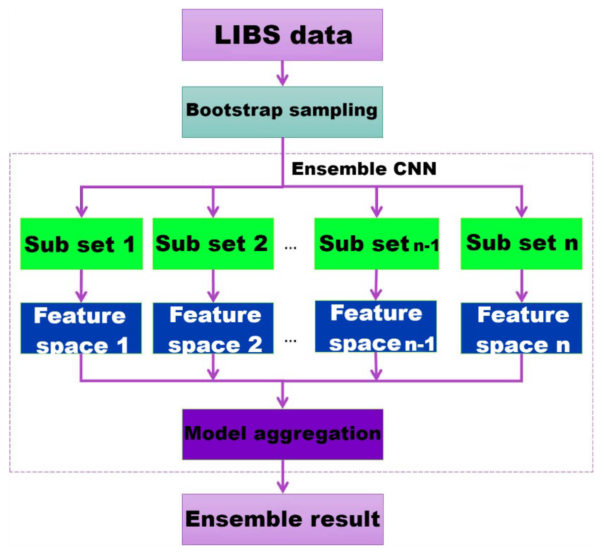
The CKW and the stride step were determined based on the length of the input spectrum and the size of the data. Due to the small data size, we selected small CKW and stride step values in this study according to a previous report [34]. As illustrated in Figure 1, the proposed CNN-based LIBS quantitative regression model consisted of five layers: input layer, convolutional layer, activation function layer, fully connected layer, and output layer; there are no pooling layers in this structure. As a substitute, we used the moving step parameters of convolutional kernels, which also reduced the output dimension of the convolutional layer. In addition, since the prediction of three major elements of LIBS belongs to the fitting (or regression) task, the output layer was set as the regression layer. It was reported that using a lightweight CNN model could enhance the performance of different spectroscopic methods [35]. Higher numbers of layers possess more parameters, so more data are required to avoid model overfitting. Notably, the gain from using CNN decreases as the complexity of the networks increases. Compared with multiple convolutional layers, the presented CNN model is parsimonious from the perspective of topological structure.
For a given spectrum, the dimension for the LIBS dataset was 6144; therefore, the input size for 1D CNN was 1 × 6144. The convolution layer was adopted to obtain the feature information of the LIBS spectrum. To capture more intrinsic properties, multiple convolutional kernels were employed in the convolutional layer. In theory, more convolutional kernels were rewarding for more features. Achieved through different kernels, the features from various categories were acquired and exploited. Simultaneously, the stride step is reduced, and the convolution kernel will extract more features. As it was a regression task, the loss function chosen was the Mean Squared Error (MSE). Additionally, the L2 norm regularization was utilized in the networks because of its ability to prevent overfitting problems. The CNN model was built based on the above steps.
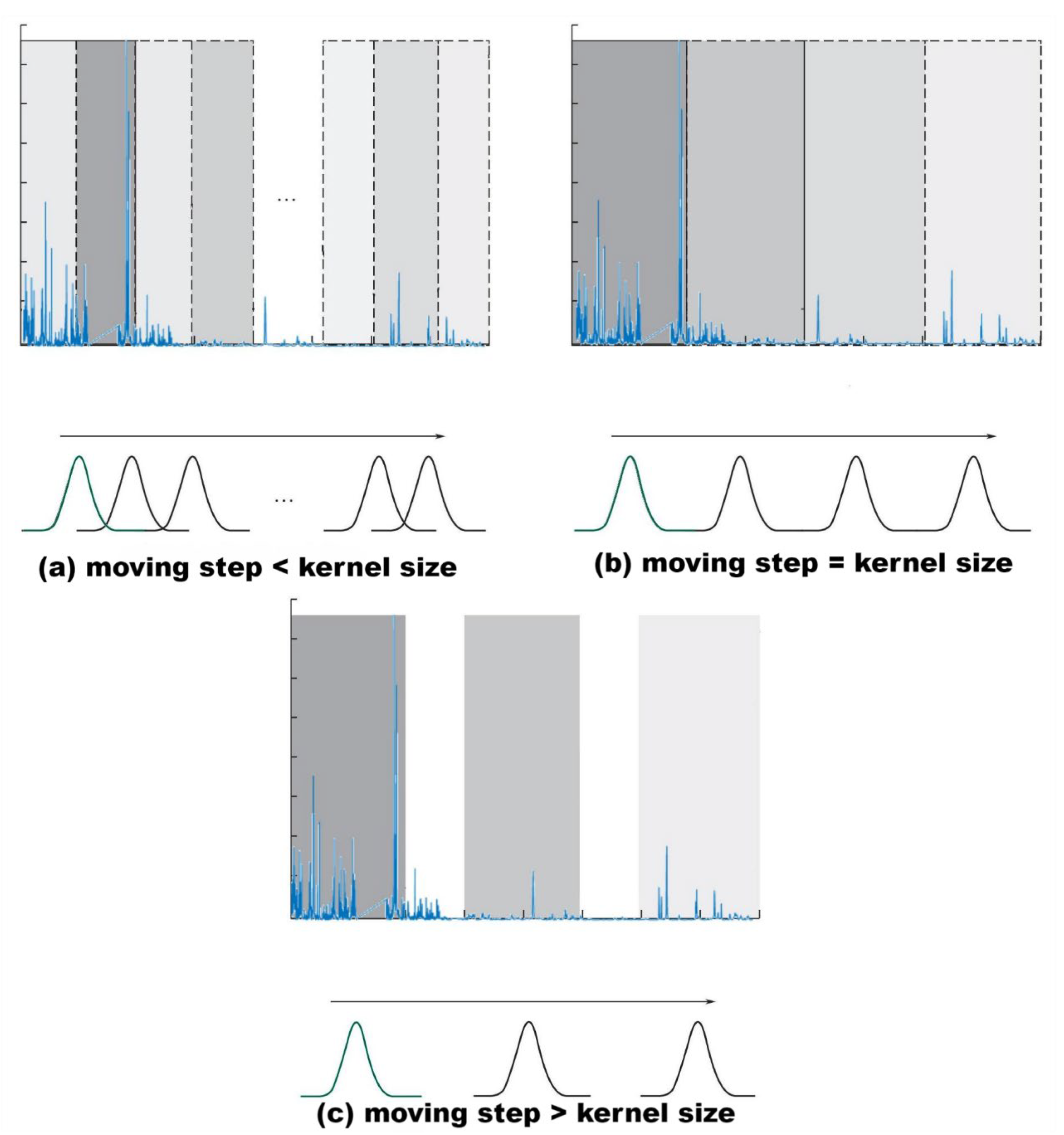
The key drawback of the CNN method is its lack of interpretation as the CNN model is considered a black box. In chemometrics, understanding the modeling and training process is as important as the results, which is why PLS is a standard method in chemometrics. Clarifying the learning mechanisms of deep neural networks, therefore, is necessary to comprehensively understand why a model produces certain outputs. In other words, to obtain a high-edge accuracy in an extremely challenging task, pure complex structures are insufficient, and an understanding of the data based on spectral expertise is essential. The wavelength interval selection method considers each wavelength interval as a unit, which improves the predictive capability, provides easier interpretation, and enables reliable calibration, such as: Moving windows PLS (MWPLS) [36], interval PLS (iPLS) [13], and synergy iPLS (SiPLS) [6]. As illustrated in Figure 2, when the stride step is smaller than the CKW, the convolution kernel overlaps with the spectral signals during movement, thus, more features can be extracted. The basic idea of obtaining overlapping spectral information derives from the MWPLS method. When the stride step is equal to the CKW, the situation is like the uniform interval division in the iPLS method. In contrast, when the stride step is bigger than the CKW, the convolution kernel skips some spectral sub-intervals and does not extract them. In other words, some useful information is lost. This situation is similar to the SiPLS method to some extent.
The proposed CNN training interpretation process exploits domain knowledge of spectroscopy variable selection to ensure model interpretability by key variables; this means that a knowledge-driven model is embedded in the nonlinear regression. Thus, the model combines the good variable interpretability of linear models and the high accuracy of nonlinear ones. In this study, we also used a visualization approach to explain the trained CNN model and present feature representations in the model. Feature map visualization is an explainable artificial intelligence method that aims to extract information from a model to improve its transparency.
Notably, the optimal result is affected by many factors, including the scale of the dataset, the structure of subnetworks, and the hyperparameters. It is difficult to establish a general guideline for determining the CNN topology. Hyperparameters including the CKW, NCK, stride step, batch size, etc., must be set before using the deep learning framework in this work. Since the training of deep learning networks is computationally expensive, the adjustment of hyperparameter combinations is not easy. In terms of systematic methods (i.e., abandoning the traditional manual trial-and-error approach), grid search is one of the most used methods for hyperparameter optimization in machine learning. Thus, inspired by existing works [37,38], a two-step progressive strategy was implemented to acquire the best parameters. First, other hyperparameter values were fixed, and a large step rough search was carried out to define the approximate search range of each hyperparameter value. Second, a small step-wise grid search was applied to achieve precise positioning of all relevant hyperparameters. The above two steps will greatly facilitate the processes of tuning the existing hyperparameters. Because they allow significant narrowing down the search space for the hidden optimal hyperparameters while still being able to explore an extensive range of different hyperparameter combinations, they are user-friendly for practitioners and experts in LIBS quantitative analysis areas.

2.3. Optimization of the CNN Analysis Model

Ensemble learning accomplishes learning tasks by building and merging multiple learners, resulting in a better prediction ability than that achieved using a single learner. Based on the generation methods of the individual learners, existing ensemble learning methods can be broadly classified into sequential methods and parallel methods. In this study, we adopted a parallel ensemble learning method considering the computational complexity. Bagging [39], which is based on bootstrap sampling, is the most well-known and representative parallel ensemble learning method, and it can be useful for regression. According to Breiman [40], “unstable” learning methods for which minor changes in the dataset can lead to significant changes in the computational results. Bagging can significantly reduce the variance of unstable processes, such as neural networks and decision trees, thus improving prediction, as averaging keeps bias constant and reduces variance. Compared with a single CNN model, bagging increases the degree of difference in model integration and improves the generalizability by reselecting the training set. However, bagging increases the computational overhead and model complexity. Of course, with the advent of GPUs, this problem has been solved. Herein, based on Breiman’s [40] finding that more than 25 bootstrap replicates is “love’s labor lost,” each ensemble model consisted of only 10 member models. The construction process of the CNN ensemble model is shown in Figure 3.
In this study, the training process of the presented approach can be summarized in three basic actions: (1) Randomly extract several data subsets from the original datasets through the bootstrap sampling (random sampling with replacement) method; (2) Construct a CNN submodel on each data subset; (3) Aggregate the CNN submodels to form an ECNN model. In the prediction stage, the outputs of 10 CNN models are aggregated into a final predictive result by applying a simple or weighted average approach. To differentiate them, we employ ECNN1 and ECNN2 to represent simple and weighted average combinations, respectively. The weights of the weighted-averaging algorithm are the normalization results of the root-mean-square error (RMSE) inverse of different weak learners in the subset. The smaller the RMSE value, the more critical the weak learner is in the final strong model. The detailed procedure can be described as follows.
Inputs: Bootstrap sampling generated K training subsets: {T1, T2, …, Tk}; the corresponding established K quantitative CNN models: {M1, M2, …, Mk}; the probed LIBS spectrum of sample i in the testing dataset: Xi.
Step 1: calculate the weights for each CNN quantitative model Mj (1 ≤ jK): {w1, w2, , wk}, where wj (1 ≤ jK) is obtained by the following Equation:
w j = S j 2 j = 1 k S j 2
where Sj is the inverse of the cross-validation error of the submodel, determined by the calibration dataset. The weights wj are restricted between 0 and 1, and the sum is normalized to 1.
Step 2: put Xi into each CNN quantitative model Mj (1 ≤ jK) and output the corresponding prediction values: {y1, y2, …, yk}.
Step 3: aggregate the predicted values for each CNN model {y1, y2, , yk} and calculate the final output of Xi:
y = j = 1 k w j y j

2.4. Quantitative Prediction Models for Comparison

In this paper, we compared three quantitative regression models (PLS [24,41], ELM [31], and CNN [13,42]), which were established based on the whole range spectra. PLS: PLS is a useful chemometrics tool for the quantitative regression of LIBS datasets [41]. In this study, the number of latent variables (LVs) employed in the PLS model was determined in the range of 5–30 through five-fold cross-validation of the training datasets. CNN: Conventional 1D CNN models were also developed for comparison. A classical network structure that was only stacked with 1D convolution layers was used. A convolutional network without pooling layers was used to avoid overfitting and to reduce the number of parameters. The structural parameters of the CNN model, including the number of convolution layers, were all optimized. ELM: The fact that the prediction ability of the BP neural network might be affected by multiple factors (e.g., the learning rate, initial weights and bias, and number of neurons in the hidden layer) was considered. The PLS model first needs to conduct LV analysis, and the number of LVs is an important parameter that requires careful testing. In contrast, the ELM model is more robust, faster, and has fewer parameters. Therefore, we selected the ELM model as a representative traditional machine learning algorithm.
Although there are a variety of modeling methods, the traditional methods are all based on the establishment of a single mathematical model and thus often fail to achieve the required accuracy and robustness. Compared to traditional modeling algorithms, the ECNN approach presented herein has the following advantages. Firstly, it is an end-to-end framework that allows the entire region of the original LIBS data as direct inputs without variable selection. When the convolutional kernel function moves throughout the entire wavelength region, it can automatically extract the local features from various data windows. Secondly, the bootstrap random sampling method ensures that the stability of the regression prediction model outperforms vanilla techniques. This is because the aggregation of “weak” CNN models is not a simple repeated average; rather, each “weak” CNN model reflects a certain local distribution of the LIBS data, thus, the aggregation result reflects the true blueprint of all the data.

2.5. Evaluation of the Prediction Model

The statistical indicators used to evaluate model performance included the root-mean-square error of cross-validation (RMSECV), the coefficient of determination of calibration (Rc2), the root-mean-square error of prediction (RMSEP), the coefficient of determination of prediction (Rp2), and the relative error rate (RER). By and large, an ideal model has low RMSEP and RMSECV, but the discrepancy between the two values cannot be significant. The higher R2 value means a better-quality model, and vice versa. Modeling and simulation were performed in the MATLAB R2019b environment (Mathworks Inc., Natick, MA, USA).
R2, RER, and RMSE are derived, respectively, as
R 2 = 1 i = 1 n ( X i Y i ) 2 i = 1 n ( X i Y ¯ i ) 2
R M S E = i = 1 n ( X i Y i ) 2 n
R E R = X i Y i X i   ×   100 %
where n is the number of samples in the calibration or prediction set, Xi and Yi are the observed and predicted concentrations of the i-th sample in the calibration or prediction set, respectively, and Y i ¯ is the mean value of the observed concentrations of all samples in the calibration or prediction dataset.

3. Results

3.1. Comparison of the ECNN Model and the Traditional Chemometric Modeling Method

In this study, the ECNN model was compared with three chemometric modeling methods commonly used in research: the PLS model, the ELM model, and the traditional CNN model. Five-fold cross-validation was used to optimize the number of LVs of the PLS model in the range of 5–30. For ELM, numerous published works [7,21,31] have demonstrated that the single hidden layer feedforward neural network can fit arbitrary nonlinear functions with zero error. Thus, cross-validation can fix the number of neurons in the hidden layer. For the CNN model, a reasonable CNN architecture was first designed, and a two-step grid search was then applied to determine the best parameters for training and finally outputting the trained model. The results of the PLS, ELM, and CNN models were all derived from the results of the above optimal models.
Overall, the RMSE of the end-to-end ECNN model proposed in this study was lower than that of the other models on the three main element datasets. In addition, the R2 value of the ECNN model was significantly better than that of the other models. Table 2 presents the RMSE and R2 values predicted by the various models on the different datasets. Due to the presence of random factors in the training process of the neural network models, each model was subjected to 25 repetitive calculations. The means and variances in Table 2 are from the results of the 25 repetitive calculations. Table 2 also lists the repeated results on the same dataset from the literature [6] to facilitate a comparison between the results obtained using the ensemble learning model and the results of previous studies. The individual member models clearly show considerable differences in the RMSEP, which implies a risk in using a single model calibration. This agrees with reports that the prediction accuracy and stability of a single model are not always convincing, especially when outliers are present or the calibration dataset is relatively small [43]. The calibration performance improves in the order of PLS < ELM < CNN < ECNN.
In the silicon (Si) content analysis, the mean RMSEP and mean Rp2 values obtained by the ECNN model were 2.3255 and 0.9686, respectively, which were superior to those obtained by the other models in this study and other models reported in the literature. The mean RMSEP obtained by the second-best performing model was 3.0451, which was 31% higher than that of the ECNN model. In the aluminum (Al) content analysis, the mean RMSEP and mean Rp2 values obtained by the ECNN model were 1.0414 and 0.9652, respectively, which were better than those of the other models in this study and the best among the results reported in the literature. The mean RMSEP obtained by the second-best model was 1.4320, which was 38% higher than that of the ECNN model. In the potassium (K) content analysis, the RMSEP obtained by the ECNN model was the smallest among the models, with a mean value of 0.3048. Compared with the next-best model, the RMSEP of the ECNN model was 48% lower, and the Rp2 was 5% higher. This indicates that the ECNN model has advantages over traditional models in practical applications. Compared to the studies employing CNN by [6,44], the 1D CNN model in our work obtained better performance, possibly due to the dimensional differences of the input spectra. Ng et al. [14] also demonstrated that a CNN model performed better with 1D spectra as the input than with 2D spectra.
Undoubtedly, the PLS presents the highest level of the linear chemometric approaches, but if there are nonlinear effects in the spectrum (generally applicable for LIBS, due to matrix effects and the fluctuation of experimental conditions, there is not a simple linear relationship between the content and the signal intensity), the performance of linear approaches will be degraded. A natural idea of this problem would result in the belief that an ANN method would perform better than PLS. However, we note that the performance of ELM and PLS predictions is neck-and-neck. The reason behind this is probably that, although ELM can handle nonlinearities, there are also some drawbacks in its application. ELM is a single hidden layer neural network where the weights between the hidden layer and input layer are randomly initialized, and the weights between the output layer and the hidden layer are calculated with a closed-form solution. This sometimes proves to be a major drawback as it increases the amount of randomness in the network, and its prediction precision is very sensitive to noise, which will lead to the results of the ELM potentially obtaining ill-conditioned solutions [45]. Under such circumstances, CNN would be a better choice because CNNs have not only great nonlinear mapping capability, but also strong tolerance to errors (spectral interference, noise, etc.). Therefore, CNN can outperform the PLS and ELM methods. Moreover, the PLS approach cannot consider the fact that LIBS data are wavelength-ordered spectra (i.e., they are in meaningful numerical order), and neither can the ELM approach. However, this fact is advantageously taken into account by the CNN. Through convolution kernel operations, the correlations between the adjacent data points in a local region can be extracted as a “feature”. Therefore, the internal correlation and unity of each spectrum are adequately exploited. This is the other reason why the CNN accuracy can outperform the PLS, and also the reason why the CNN can behave better than ELM. The CNN prediction model shows less fluctuation than the ELM prediction model, which may be attributed to the fact that some convolutional kernels have a smoothing function in the CNN model training (see Section 3.3), reducing part of the spectral noise. The excellent performance of the CNN quantitative model indicates that CNN can successfully suppress the chemical matrix effect and can be employed for the LIBS quantification of 1D ChemCam spectra data.
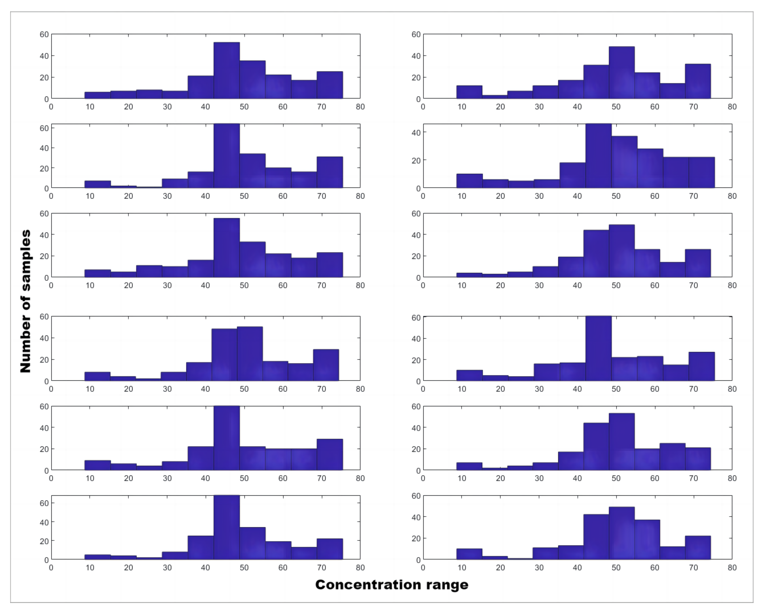
Here, we explore why the proposed ECNN network achieves better prediction ability than traditional techniques. In the field of machine learning, data are usually divided into training, validation, and testing datasets. Nevertheless, the entire LIBS data distribution may differ from those of the three subsets, suggesting that the model built with the training dataset may not be suitable for the testing or validation dataset. The presented ECNN introduces the idea of ensemble learning, which combines many “weak” models to establish a “strong” model. The weak models were built with different training datasets (rather than simply repeating them). Figure 4 shows the results of a randomized trial conducted using the bootstrap sampling strategy. It is easy to see that each trial’s distribution was different, indicating that each weak model has limitations since it cannot process the entire dataset. From another perspective, we can infer that each weak model has its own specialty since each weak model is sufficiently efficient to process local parts of the entire dataset. The presented ECNN combined several weak models to form a strong model that could cover all of the LIBS data. This can be explained as follows: Before establishing a member model, the bootstrap sampling strategy results in multiple versions of the training dataset, on which the ECNN can obtain various modeling subspaces. The random operations built in the ECNN and the differences introduced by the bootstrap strategy might introduce the diversity for ensemble modeling. The combination of these methods successfully maintains an appropriate diversity among member models and aggregates the feature information on both the shapes and heights of the spectral lines, improving the calibration.
We also note that the performance of the calibration model is related to different input sizes and weight optimization methods. A noteworthy point is that in the ECNN1, all the submodels are assigned equal weights in training, but such an equal-weight strategy may not be good enough for the quantification task. The weight is a measure of how well each subset of the spectrum correlates with the target attribute. Since the characteristic peak intensities are crucial to LIBS quantitative analysis, it might be better and more dependable if the learned weights from the training data are highlighted. This idea can be compared to the process of consulting several experts to make a final decision. From another perspective, although CNN has strong learning capabilities, without the contribution of an appropriate amount of data, the ability to realize superior performance may be hindered. The accuracy advantage of ECNN compared to other methods is again increased with the increasing sample size of the training dataset. This suggests that the increased sample size would enhance the ECNN model to learn useful information from multiple spectra sources. Some authors [2,46] have observed the trend of plateauing of the performance (maximized up to a certain point) with an increasing sample size. This trend is associated with model complexity, as simpler models (e.g., PLS) cannot reflect all the variation in the spectra. Therefore, more complex, nonlinear models are appropriate when the sample size is larger. As the sample size increases, the ECNN model can better characterize the structure of LIBS spectra.
In addition to testing the specific values of R2 and RMSE, we also performed a relative error analysis to make the comparison statistically significant. To intuitively evaluate the quantitative accuracy of these methods, the absolute value of the prediction RER was calculated for each element using Equation (5), and the RER value is in units of %. We have chosen to show the following LIBS samples: Norite, Picrite, Shergottite, NAU2-LO-S, NAU2-MED-S, and KGA-MED-S. These standards were chosen because they are ChemCam calibration target samples (CCCT, the onboard Curiosity rover calibration target), as reported by Wiens et al. [32].
The concentration RERs for all six validation examples from the expanded dataset are displayed in Table 3. From a global view, each method successfully predicted the concentration of most samples and was pretty close to the “actual” values. We also observe that when the calibration data is sufficient, the ECNN model can provide the best individual and overall accuracy in most validation examples. For the three silicate glasses (Shergottite, Picrite, and Norite), the predicted values of all methods were close to the true values. In addition, the predicted results of the ECNN were closer to the true values than others. For the three ceramic targets (NAU2-LO-S, NAU2-MED-S, and KGA-MED-S), our quantification results and other result values were both higher than the true values acquired in the scientific laboratory, which can be attributed to two aspects: (1) The NAU2-LO-S, NAU2-MED-S, and KGA-MED-S are sulfate-bearing targets, including sulfate, basalt, and clay, and complex matrix effects cause lower prediction accuracy. (2) The ChemCam igneous samples are less heterogeneous than ceramic samples. As mentioned by Clegg et al. [33], the KGA-MED-S spectrum recorded on Martian even showed some additional emission lines, including Mg (280, 285 nm) and Ca (315, 317, 393, 396, 422 nm) compared with those recorded in the laboratory on Earth. This may imply challenges for the quantification analysis of volatile-rich and heterogeneous standards.
Although the low RERs of each method seem to be “satisfactory”, it is also worth noting that there are cases where the RERs calculated exceed 40%. Such situations usually occur when the actual concentration values are extremely small (around 0.5% or even less), such as the K element in NAU2-LO-S and NAU2-MED-S samples. This phenomenon is present in all data, and can only be well explained by a more in-depth examination of the properties of the spectral data themselves. On the one hand, the above results show that the ensemble can significantly increase the accuracy of the CNN submodels, such as Al and Si elements. This is because these elements have a wider compositional range, are more sensitive to submodel demarcation, and the effects of ensemble optimization are better than those of the non-optimization methods. On the other hand, the composition of K is mostly distributed below 10%, therefore, whether or not to generate the subset might have less impact on such elements. If the standards contain relatively concentrated compositions, the optimization of elements is effective but not very obvious.
Undoubtedly, the CNN and ECNN models are superior to the ELM and PLS models. We owe these phenomena to the powerful feature extraction ability of the CNN model. The CNN method can yield the second-best RER, but its superiority over PLS and ELM models becomes less prominent than ECNN. It can be found that, in most cases, the RER of ECNN is one or two orders of magnitude improvement than that of other methods. Specifically, most of the RERs are at 10% order of magnitude for the ELM and PLS. For CNN, the lowest RER is at 1% order of magnitude. While for the ECNN, the lowest RER can reach 0.1% order of magnitude, such as Si and Al in the NAU2-LO-S sample and Si in the Shergottite sample. It was largely ascribed to the ingenious combination of CNN and other data mining methods. The basic CNN is still able to predict element concentrations at a time from one model, so it is worth trying to modify the training mode of the CNN. Ensemble learning is a novel machine learning approach that employs multiple submodels instead of a single model to address specific problems. It enables the CNN model to learn more of the common spectral features from various data sources, thereby improving the robustness and accuracy of the CNN model and making its performance much better than traditional models. Thus, for big-data environments, the ECNN is a more effective spectral regression modeling method that can make more accurate predictions. Although the ECNN method showed advantages over the other three approaches, we have to look straight at the reality that its quantitative predictive results are still far from satisfactory. The most common absolute value of relative error is around 10%, which means that room for improvement remains.
Besides increasing the diversity and quantity of the training samples, it is also crucial to carefully build a suitable training dataset. There is an empirical rule for LIBS quantitative analysis that the target sample with the lowest concentration and that with the highest concentration should only be used as training samples. In some research, e.g., [4,17,47], the entire dataset was randomly divided, and the rules were ignored. However, we recommend using a carefully designed partitioning mode to make the data in each set more representative and thus facilitate network learning. Otherwise, it might predict negative or zero values for some low-concentration targets, thus increasing the error of the RER.

3.2. Influence of CNN Parameter Values on the Predictive Ability of the Model

As with other CNN-based applications, there is a strong relationship between the predictive performance of the quantitative model and the CNN parameter values. In this work, due to the limited space, we used the R2 of Si only as an example to demonstrate the influence of NCK, CKW, mini-batch size, and stride-step size on the predictive ability of the model. Si is an essential element for understanding both sedimentary and igneous geochemistry. Further extensions of the hyperparameter analyses are listed in Appendix A.

3.3. Visualization of Features Extracted by the CNN Network

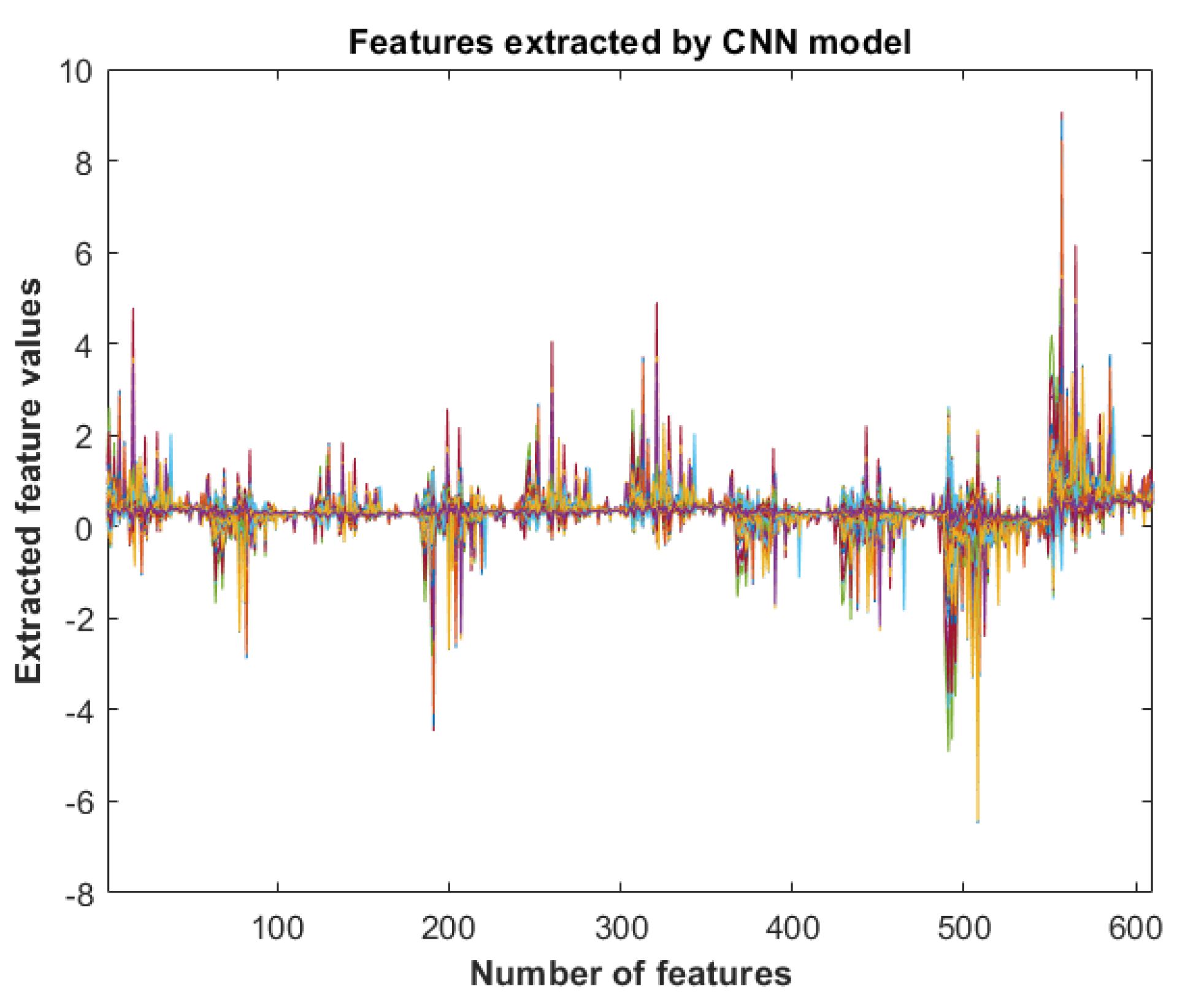
The visualization of feature maps provides insights into data transformations through the convolutional layers in a CNN model. Generally, the deeper the layer is, the more complex features it learns. For CNN frameworks with two or more convolutional layers, the input LIBS data is compacted into increasingly complex abstractions from layer to layer, and it may not be possible to trace back which features of the last convolutional layer map was placed into which input variables. In the special situation of the presented 1D CNN model, only one convolution layer exists. This shallow structure allows the model to provide a more straightforward correlation between the input spectrum region and the 1D representation of the activation, since each filter neuron is the result of neighboring input neurons. Consequently, this approach lets us directly visualize which parts of the spectral data are considered vital with potentially only slight drifts. Here, Al is taken as an example for detailed discussion. The correspondence between the abstract features extracted with the CNN and the feature emission lines of the original LIBS data is illustrated in Figure 5, which shows good consistency (281–282.5 nm, 288–288.5 nm, 308–310 nm, 394–395 nm, 395.5–397 nm). The convolution layer is used for spectra pre-processing and learns the spectral shape features. Almost all the feature maps have similar peak shapes to the raw input spectra. Simultaneously, we attempt to explain the results from another angle. As illustrated in Figure 6, 610 abstract features were captured from 10 convolution kernels. The abstract features were automatically clustered into 10 groups, consistent with the 10 convolutional kernels. Some kernels captured the differences between samples, while others could not. Each convolution kernel extracted characteristics of interest from a specific angle, consistent with existing research [48] in image processing.
The shapes of the convolutional kernels with different kernel sizes are illustrated in Figure 7. The visualization results of the convolutional filters agree with the findings of a previous study [35]. Filters containing many non-zero elements and linear trends of intensity show similar effects of smoothing and derivatives, and the well-trained convolutional model can replace the traditional pre-processing methods for spectra analysis.

4. Discussion

4.1. Model Design

Designing a CNN is a frequently repetitive process that involves the selection of various parameters, including the number and types of layers and the learning rate. When building a model, various parameters must be comprehensively considered and analyzed because they significantly impact the model and its prediction performance. We therefore intend to present the best practice model optimization approach according to the obtained results.

4.1.1. Number of Network Layers

The data sizes of publicly available datasets range from 56 to 81,840 but are less than 1000 for most datasets. Studies have shown that a 10-layer neural network model is sufficient to successfully extract the hidden spectral features [49]. In general, the larger the input sample size, the deeper the model. Currently, the most used neural network model structure is composed of two to three convolutional layers and one or two fully connected layers.

4.1.2. Effects of Convolution Kernel Parameters

According to Ng et al. [46], a convolution kernel is a weight matrix used for feature detection that determines the size of the output feature map. Although the NCK varies greatly among studies, the change in NCK has been reported to be closely related to the sample size. A large dataset provides support for training many parameters. For example, the training sets in Refs. [50,51] each contained more than 10,000 samples, and the corresponding NCK values were also large.
Notably, the CKW and stride step must be assigned values by the user when defining the CNN topology. In line with data processing for other 1D spectra [52], we think that the relationship between CKW and stride step has a clear physical meaning when analyzing atomic spectra. When setting the model parameters, the stride step should not exceed the CKW to avoid information loss. In addition, the optimal CKW must be continuously verified by testing to find the most suitable range. It is unwise to conclude that one method is superior or inferior to another because the performance of a chemometric algorithm genuinely depends on the specific dataset used. There is no universal “best” method, but there may be a most “suitable” method for a given problem. Only more experiments and experience can continuously explore a more optimal combination [53]. For example, when the size of input samples is large, pooling and convolutional layers need to be appropriately added to create a deep CNN. While the background of input wavelengths is complicated in the context, the NCK can be increased, allowing the model to extract more features.

4.2. Understanding the Models

In line with the old saying that “there is no free lunch,” when applying the presented ECNN, one must be aware of its costs and benefits. The end-to-end attributes function as information distillation pipelines to enhance informative variables, extract overall features, and directly filter out irrelevant information. The feature map truly corresponds to the input spectrum owing to the spatial invariance of the CNN. However, as mentioned earlier, the convolution kernel and the extracted features are abstract, resulting in features quite different from the frequency- or time-domain features obtained using traditional techniques. Stacking [25,29] is one of the ensemble learning methods. It can integrate model strategies based on wavelength range selection, where several different wavelength ranges are selected to build submodels for simultaneous prediction. From another point of view, we note that some intervals are assigned smaller weights, and this idea is valuable. Stacking methods consider not directly removing the intervals that contribute little to the iteration and optimization processes. Instead, such intervals would be assigned smaller weights, and thus, useful information is retained. Stacking has been proven successful in applications involving other 1D spectral data. How to further interpret these abstract shapes and more features of high-dimensional LIBS data, however, remains an open challenge that requires more research.
In addition, the number of submodels T is an important parameter that dramatically affects the ensemble model’s prediction results. When T is too large, the predictive accuracy is appealing, but the model computation time is longer. With too small T, the superiority of ensemble modeling cannot be demonstrated, and the corresponding predictive accuracy will be poor. Therefore, it is important to determine a proper T for the ensemble. This work sets the value to 10 because the saturation phenomenon will appear when the value is greater than 10.

4.3. Future Development Trends

Although the current models developed for the major elements are acceptable, they could be improved. Based on the results, further research can be conducted in the following aspects:
  • Consider the measurement uncertainty that affects the results of the models: In several remote LIBS measurements, such as ChemCam, issues that limit the accuracy and precision of the elemental composition of targets are not necessarily related to the post processing of the data, but in some cases with the experimental conditions [54,55]. The proposed method should be tried out for more than just the chemical matrix effect, such as with different sample states, variable laser-target distances, etc.
  • Implement data augmentation algorithms: As demonstrated in the part of the results section, a large enough training set size is crucial to the CNN model. However, as can be seen from Table 1, after the size of the calibration dataset was expanded, the range of the three elements was also greatly expanded. The most intuitive tendency may be the diversification of the samples in LIBS detection. The fine distinction between the sample quantity and the sample material diversity should be noted. In actual situations, the dataset is usually unbalanced and limited. Thus, the number of samples available for calibration modeling may be limited. In fact, this problem should be fundamentally solved by increasing the number of training samples for each material, that is, data augmentation. The augmentation simulates slightly different spectral acquisition scenarios (e.g., instrumental offset, background lighting, etc.) so that they created multiple (slightly different) copies of the original spectrum for the same target value. The training sample dataset can be remarkably expanded so the models can become robust to unseen variations. Actually, the problem of small dataset learning occurs in various practical applications [56,57,58], which confirms that the model which was established based on the original small dataset may not be inapplicable when predicting future samples, since they are also valid data. Thus, in our future work, we will try to fill the information gaps by systematically generating virtual samples.
  • Design of lightweight models: Hardware deployment for lightweight models is also an important future research direction for Mars rovers. The CNN spectral analysis method is combined with portable hardware [36,59,60] to promote the practical application of portable spectrometers in various fields. Two-dimensional CNNs have unique advantages in image feature extraction, but 1D CNNs are better matches in terms of dimensionality. In addition, 1D CNN models have more compact structures and lower hardware requirements, making real-time, efficient, and low-cost complete configurations possible. Therefore, the authors would like to emphasize that the simpler the model, the easier it is to utilize and interpret in practical situations [61,62]. For example, to deploy a computational model in a realistic Mars environment, it is much more desirable to have a lighter, simpler model that can run on modest microprocessors than a highly complex architecture that demands more computation cost.

5. Conclusions

Deep learning methods have great application potential in spectroscopy analysis. To better satisfy the current demands of Earth–Mars spectral correction for analyzing the Mars surface composition, we examined deep learning-based spectral analysis methods and their mechanisms, and constructed an end-to-end ECNN spectral data analysis system. The experimental results for three elements of datasets with different sizes indicated that the presented ECNN outperformed traditional techniques (single-CNN, ELM, and PLS models) in terms of prediction performance. This study also provides an understanding of the CNN training interpretation process based on spectral expertise along with insights into the data transformations performed in the CNN model through feature map visualization. These findings are useful for dealing with the tricks of topology pruning and parameter tuning and for uncovering the interpretable principles of CNN. In summary, the results indicate that the presented ECNN method simplifies the feature selection process required by traditional chemometric methods, improves the accuracy and robustness of spectral analysis, reduces the risk of model overfitting, and provides a more reliable general spectral analysis strategy for technicians in related industries.

Author Contributions

Conceptualization, Y.Y. and M.Y.; methodology, Y.Y.; software, Y.Y.; validation, Y.Y.; formal analysis, Y.Y.; investigation, Y.Y.; resources, M.Y.; data curation, M.Y.; writing—original draft preparation, Y.Y.; writing—review and editing, Y.Y.; visualization, Y.Y.; supervision, M.Y.; project administration, Y.Y.; funding acquisition, M.Y. All authors have read and agreed to the published version of the manuscript.

Funding

This work was sponsored by the National Natural Science Foundation of China (NSFC) through grants No. 62103163 and No. 62003055, and Natural Science Foundation of Jilin Province through grant No. YDZJ202101ZYTS033. We thank the above-mentioned funds for their financial support.

Data Availability Statement

The spectra used in this study are available for downloading from the NASA Planetary Data System at http://pds-geosciences.wustl.edu/missions/msl/chemcam.htm (accessed on 4 July 2023).

Acknowledgments

The authors would like to thank Lei Yu from Shanxi University, Jipeng Huang from Northeast Normal University, and Xueming Xiao from Changchun University of Science and Technology for fruitful discussions on the model.

Conflicts of Interest

The authors declare no conflict of interest.

Appendix A. Hyperparameter Selection

  • Effect of CKW on the Generalizability of the Prediction Model
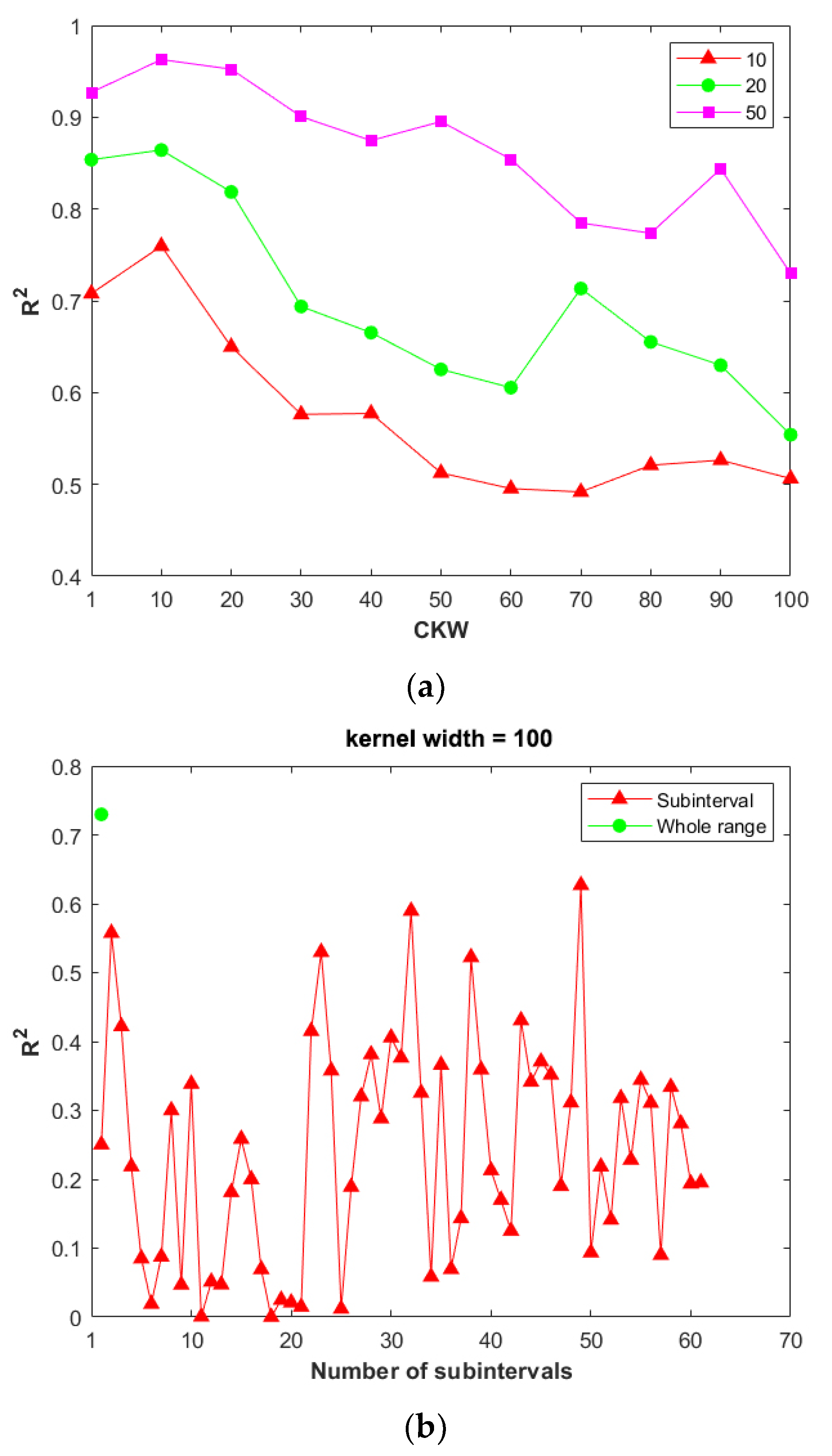
Previous research across many fields has demonstrated that the CKW significantly influences pattern (feature) extraction and subsequent calibration modeling. If the CKW is too large, the obtained characteristics might contain noisy and redundant data. Conversely, if the CKW is too small, the complete scene of certain patterns cannot be extracted. Similarly, in LIBS data analysis cases, a small CKW may not cover the waveband near the feature emission lines. In contrast, a large CKW may result in the selection of unnecessary features, in addition to the emission lines near characteristics, which could influence the prediction ability of the regression model.
Figure A1 shows the prediction model results when the NCK was fixed at 10, 20, and 50. (In these protocols, CKW was equal to the stride step, corresponding to no overlap between different sub-intervals.) It is worth mentioning that the unit of CKW here is the number of variables rather than nm. Considering that the LIBS data include only 240 observations, this means that the number of samples is much lower than the number of features. If all these characteristics are employed to build a regression model (first column in Figure A1a), the Rp2 of the prediction model is slightly lower than when CKW = 10. The other point that must be considered is that when CKW is equal to the stride step, it is equivalent to dividing the full spectrum of original LIBS data into certain subintervals on average. When the extracted features from each subinterval were used to build a prediction model (red triangles in Figure A1b), Rp2 was different between the subintervals. In summary, modeling using features from a particular subinterval, or all features, is not preferred, and it is necessary to identify the optimal combination of parameters prior to modeling.
Figure A1. Effect of CKW on the model’s prediction ability: (a) NCK = 10, 20, 50; (b) kernel width = 100.
Remotesensing 15 03422 g0a1
2.
Effect of NCK on the Generalizability of the Prediction Model
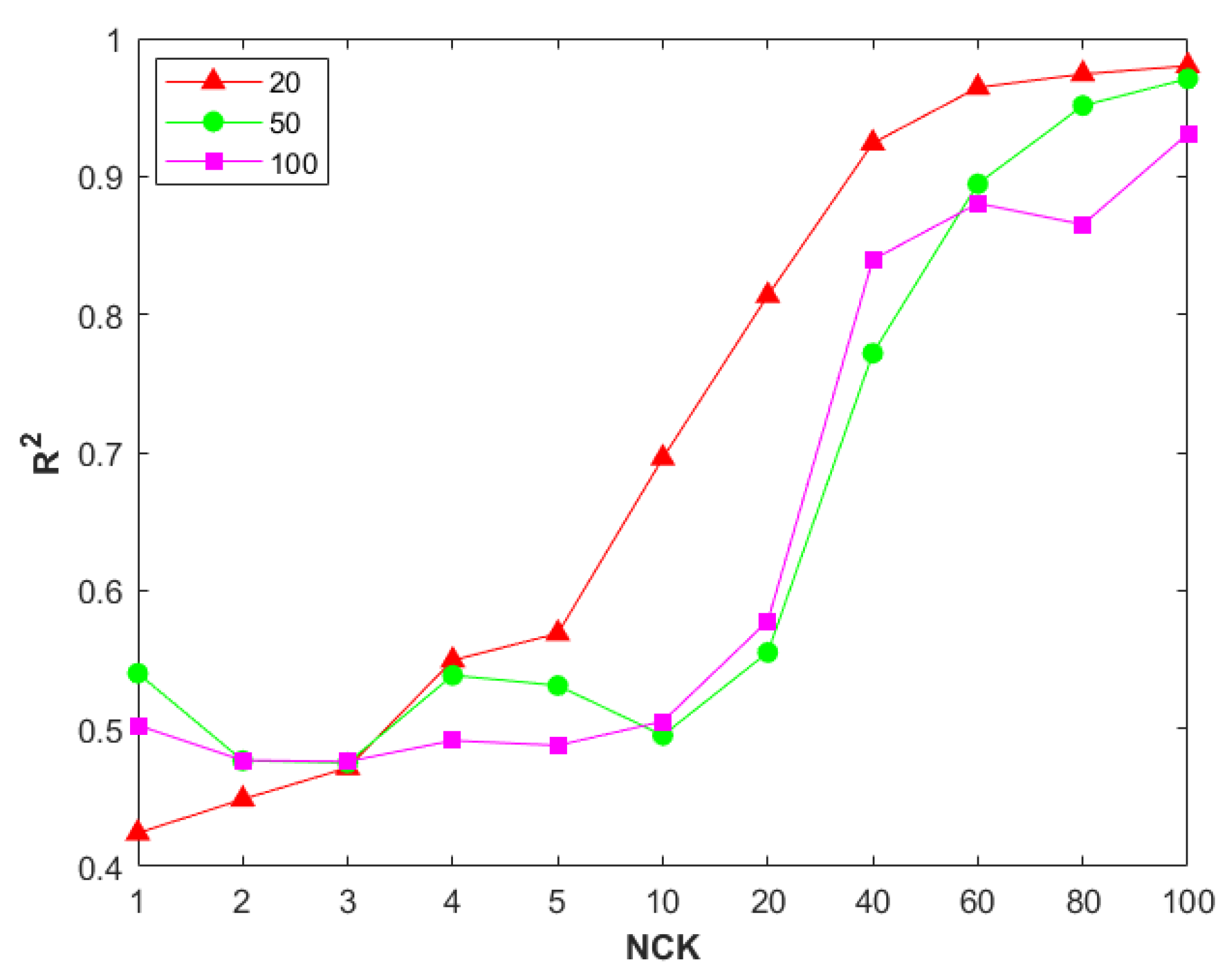
In theory, a larger NCK allows us to capture the inherent characteristics of raw LIBS data from multiple dimensions. Nevertheless, when the NCK increases, the number of extracted characteristics increases at the same time. For instance, assuming that the stride step and CKW are equally fixed to 100, when a convolutional kernel moves through the LIBS waveband region, it will generate 61 (6144/100) features; therefore, M convolutional kernels will result in 61×M features. The effects of the NCK on the generalizability of the calibration model are shown in Figure A2, which clearly shows the following: (1) when CKW was small (e.g., 20 or 50, as shown by the red triangles and green dots in Figure A2, respectively), NCK increased, Rp2 first increased significantly and then stabilized; (2) when CKW was large (e.g., 100, purple squares in Figure A2), Rp2 increased significantly as NCK increased from 5 to 60 and then decreased slightly when NCK further increased to 80. Thus, the generalizability of the prediction model was affected by the coupling between the CKW and NCK.
Figure A2. Effect of NCK on the model’s prediction ability.
Remotesensing 15 03422 g0a2
3.
Effect of Stride Step on the Generalizability of the Prediction Model
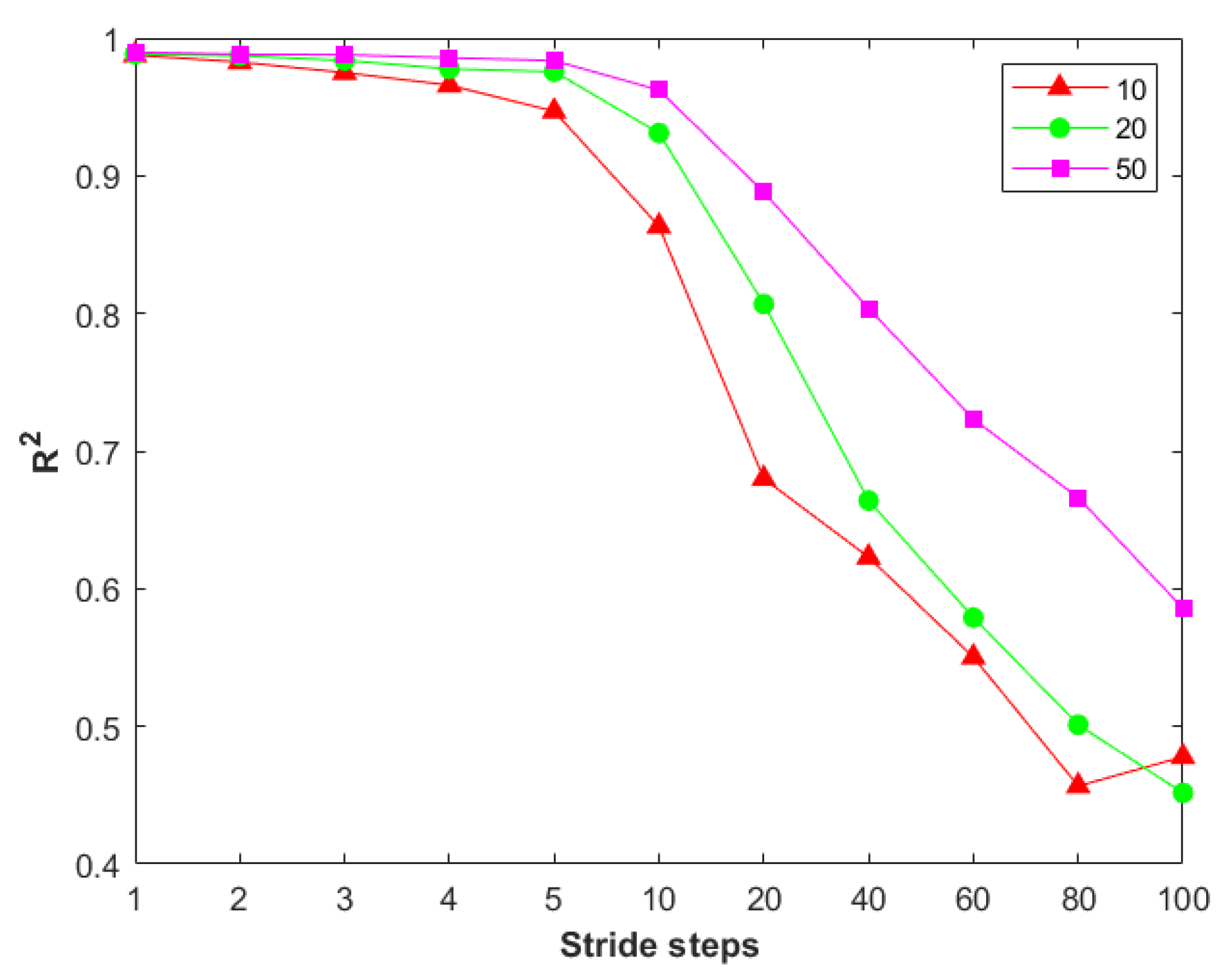
As mentioned above, when the CKW is the same as the stride step, it is equivalent to dividing the entire region of the original LIBS data into certain sub-intervals on average. Nevertheless, in some cases, the feature emission lines may be located at the edges of two neighboring sub-intervals, which will prevent the convolutional kernel from collecting intrinsic knowledge in the vicinity of the feature emission lines. Reducing the stride step might be a promising way to address this issue. Figure A3 illustrates the effect of stride step on the prediction ability of the models for CKW = 10, 20, and 50 and NCK = 20. When the stride step is smaller than CKW, the entire region of LIBS data can be divided into overlapping subintervals. In addition, the consideration of this overlap improves the prediction ability of the calibrated model. For instance, consider the case of the feature emission line at 288.24 nm. When both the CKW and the stride step are set to 20, the corresponding subinterval is 288.15–289.14 nm. When the stride step is 10, the corresponding subintervals are 287.66–288.64 nm and 288.15–289.14 nm. The Rp2 values of the model with extracted characteristics in these two cases are 0.6639 and 0.6906, respectively, indicating that small stride steps (stride step < CKW) are beneficial for enabling the convolutional kernels to capture characteristics near these feature emission lines. Comparable results were also obtained for the other parameters in Figure A3.
Figure A3. Effect of stride step on the model’s prediction ability.
Remotesensing 15 03422 g0a3
4.
Effect of Mini-Batch Size on the Generalizability of the Prediction Model
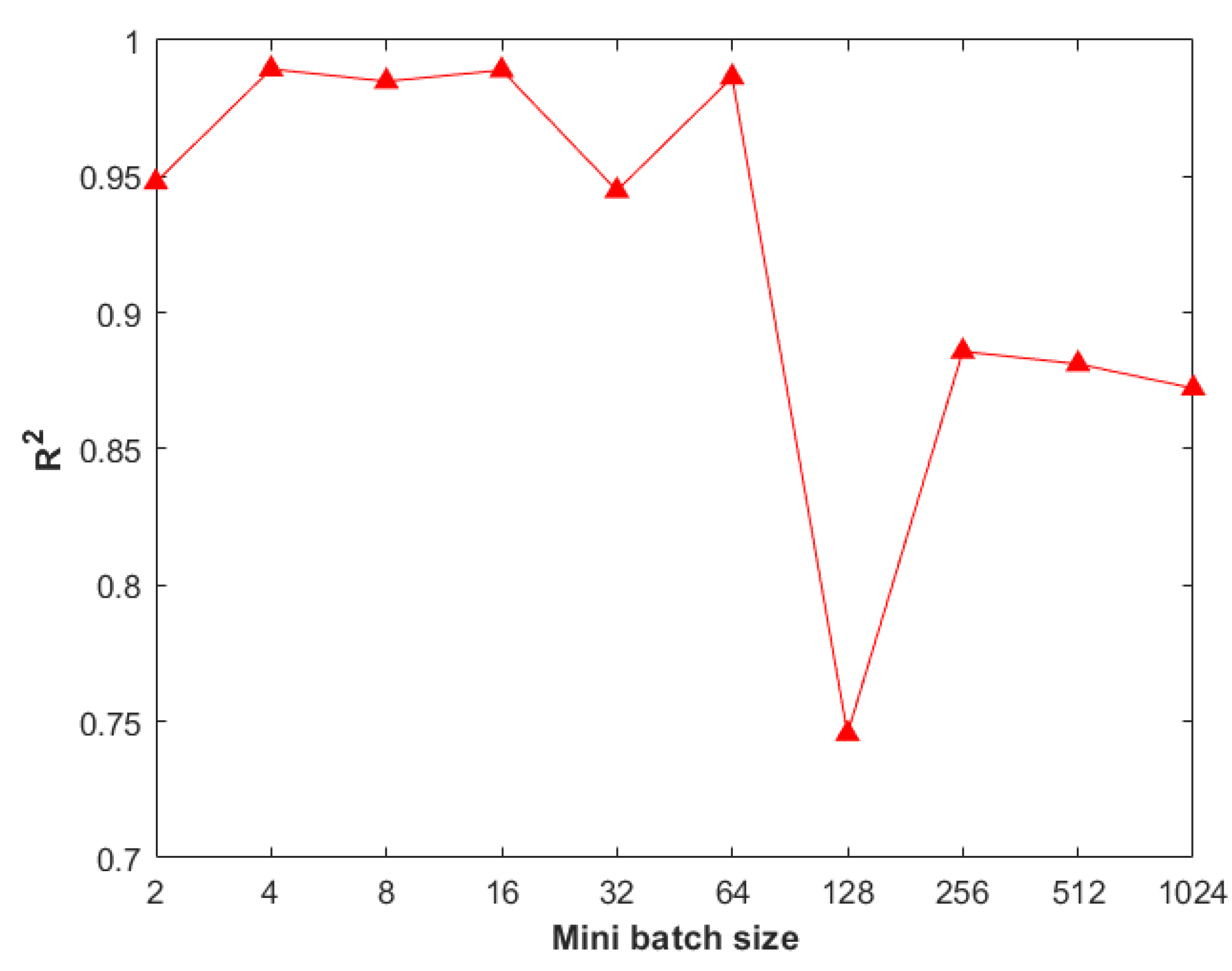
The effect of the mini-batch size on the predictive ability of the model was evaluated when the stride size, CKW, NCK, and max epochs were set to 1, 10, 50, and 2000, respectively. As shown in Figure A4, when the mini-batch size was around 100, Rp2 tended to be saturated, indicating that the CNN model was sufficiently trained for prediction. However, as the mini-batch size increased, Rp2 decreased. This might be due to the small number of samples in the training dataset (around 200 × 0.632~126); increasing the mini-batch size reduced the number of updates of convolution kernel parameters in each iterative epoch.
Figure A4. Effect of mini-batch size on the model’s prediction ability.
Remotesensing 15 03422 g0a4
5.
Paradigm for the Overall Design of CNN Parameters
Parameter tuning, which is the key to deep neural network performance, is the most cumbersome step and requires constant trial-and-error. The parameters that must be manually set in a CNN model usually include CKW, NCK, and stride step. At present, there is no satisfactory theory to guide the determination of the various parameters in ANN algorithms, which is indeed a general limitation and flaw of ANNs. We think that the above three parameters have nonmonotonic relationships with model performance (not “the larger the better” or “the smaller the better”). Moreover, the three parameters are not completely independent; instead, they have mutually coupled relationships. Based on the above series of experimental studies, the design paradigm for the CNN model parameters in LIBS analysis cases is summarized as follows.
(1)
The CKW should not be too small. If the CKW is too small, the convolution kernel extracts the characteristics in some subintervals that are not near the characteristic spectral line, and the model constructed based on these features usually has poor generalization performance. When the CKW is moderate, each feature captured by the convolution kernel contains spectral information near the characteristic spectral line, and the model constructed from these features usually has good generalization performance.
(2)
The NCK should not be too large. When the CKW is small, the number of features captured by a single convolution kernel is relatively large. In this case, if the NCK is continuously increased, the total number of features captured by all the convolution kernels will double, and the number of features will vastly exceed the number of samples, causing overfitting and a gradual decrease in the model’s predictive performance. In contrast, when the CKW is large, the model’s predictive performance increases, and after the NCK reaches a threshold value, further increasing the NCK slightly reduces the model’s predictive performance. Therefore, a higher NCK value is not necessarily better. When the CKW value is appropriate, the NCK should not exceed 60.
(3)
The stride step should be smaller than the CKW. When the stride step is small, more characteristics can be captured, which helps enhance the model’s prediction ability.

References

  1. Caceres, J.O.; Sainz de los Terreros, J.Y. A real-world approach to identifying animal bones and Lower Pleistocene fossils by laser induced breakdown spectroscopy. Talanta 2021, 235, 122780. [Google Scholar] [CrossRef] [PubMed]
  2. Li, L.-N.; Liu, X.-F.; Yang, F.; Xu, W.-M.; Wang, J.-Y.; Shu, R. A review of artificial neural network based chemometrics applied in laser-induced breakdown spectroscopy analysis. Spectrochim. Acta Part B-At. Spectrosc. 2021, 180, 106183. [Google Scholar] [CrossRef]
  3. Guo, K.-C.; Wu, Z.-C.; Zhu, X.-P.; Ling, Z.-C.; Zhang, J.; Li, Y.; Qian, M.-C. Mineral element abundance identification based on libs emission line selection by loading space distance of principal component analysis. Acta Photonica Sin. 2019, 48, 1030002. [Google Scholar] [CrossRef]
  4. Chen, S.; Pei, H.; Pisonero, J.; Yang, S.; Fan, Q.; Wang, X.; Duan, Y. Simultaneous determination of lithology and major elements in rocks using laser-induced breakdown spectroscopy (LIBS) coupled with a deep convolutional neural network. J. Anal. At. Spectrom. 2022, 37, 508–516. [Google Scholar] [CrossRef]
  5. Fabre, C.; Ourti, N.E.; Ballouard, C.; Mercadier, J.; Cauzid, J. Handheld LIBS analysis for in situ quantification of Li and detection of the trace elements (Be, Rb and Cs). J. Geochem. Explor. 2022, 236, 106979. [Google Scholar] [CrossRef]
  6. Yu, Y.; Yao, M.; Huang, J. A hybrid wavelength selection strategy-based quantitative analysis model for LIBS data from standard ground samples of the Curiosity rover on Mars. J. Anal. At. Spectrom. 2022, 37, 2362–2376. [Google Scholar] [CrossRef]
  7. Zhang, Y.; Huang, J.; Zhang, Q.; Liu, J.; Meng, Y.; Yu, Y. Nondestructive determination of SSC in an apple by using a portable near-infrared spectroscopy system. Appl. Opt. 2022, 61, 3419–3428. [Google Scholar] [CrossRef] [PubMed]
  8. El Haddad, J.; Bruyere, D.; Ismael, A.; Gallou, G.; Laperche, V.; Michel, K.; Canioni, L.; Bousquet, B. Application of a series of artificial neural networks to on-site quantitative analysis of lead into real soil samples by laser induced breakdown spectroscopy. Spectrochim. Acta Part B-At. Spectrosc. 2014, 97, 57–64. [Google Scholar] [CrossRef] [Green Version]
  9. Cui, W.; Hao, Y.; Xu, X.; Feng, Z.; Zhao, H.; Xia, C.; Wang, J. Remote Sensing Scene Graph and Knowledge Graph Matching with Parallel Walking Algorithm. Remote Sens. 2022, 14, 4872. [Google Scholar] [CrossRef]
  10. Song, W.; Afgan, M.S.; Yun, Y.-H.; Wang, H.; Cui, J.; Gu, W.; Hou, Z.; Wang, Z. Spectral knowledge-based regression for laser-induced breakdown spectroscopy quantitative analysis. Expert Syst. Appl. 2022, 205, 117756. [Google Scholar] [CrossRef]
  11. Ge, Y.; Zhang, X.; Atkinson, P.M.; Stein, A.; Li, L. Geoscience-aware deep learning: A new paradigm for remote sensing. Sci. Remote Sens. 2022, 5, 100047. [Google Scholar] [CrossRef]
  12. Hsu, C.-Y.; Li, W.; Wang, S. Knowledge-driven GeoAI: Integrating spatial knowledge into multi-scale deep learning for Mars Crater detection. Remote Sens. 2021, 13, 2116. [Google Scholar] [CrossRef]
  13. Chen, Y.Y.; Wang, Z.B. End-to-end quantitative analysis modeling of near-infrared spectroscopy based on convolutional neural network. J. Chemom. 2019, 33, e3122. [Google Scholar] [CrossRef]
  14. Ng, W.; Minasny, B.; Montazerolghaem, M.; Padarian, J.; Ferguson, R.; Bailey, S.; McBratney, A.B. Convolutional neural network for simultaneous prediction of several soil properties using visible/near-infrared, mid-infrared, and their combined spectra. Geoderma 2019, 352, 251–267. [Google Scholar] [CrossRef]
  15. Cai, Y.; Li, S.; Yao, Z.; Li, T.; Wang, Q. Online detection of concentrate grade in the antimony flotation process based on in situ Raman spectroscopy combined with a CNN-GRU hybrid model. Spectrochim. Acta Part A Mol. Biomol. Spectrosc. 2023, 301, 122909. [Google Scholar] [CrossRef]
  16. Xueqiang, C.; Zhang, L.; Zhongchen, W.; Zongcheng, L.; Jialun, L.; Kaichen, G. Quantitative analysis modeling for the ChemCam spectral data based on laser-induced breakdown spectroscopy using convolutional neural network. Plasma Sci. Technol. 2020, 22, 115502. [Google Scholar]
  17. Pengfei, Z.; Ting, Z.; Daohua, X.; Li, Z. Quantitative analysis research of ChemCam-LIBS spectral data of Curiosity rover. Infrared Laser Eng. 2022, 51, 323–332. [Google Scholar]
  18. Li, L.-N.; Liu, X.-F.; Xu, W.-M.; Wang, J.-Y.; Shu, R. A laser-induced breakdown spectroscopy multi-component quantitative analytical method based on a deep convolutional neural network. Spectrochim. Acta Part B At. Spectrosc. 2020, 169, 105850. [Google Scholar] [CrossRef]
  19. Chen, Y.-Y.; Wang, Z.-B. Quantitative analysis modeling of infrared spectroscopy based on ensemble convolutional neural networks. Chemom. Intell. Lab. Syst. 2018, 181, 1–10. [Google Scholar] [CrossRef]
  20. Chen, Y.-Y.; Wang, Z.-B. Feature selection based convolutional neural network pruning and its application in calibration modeling for NIR spectroscopy. Chemom. Intell. Lab. Syst. 2019, 191, 103–108. [Google Scholar] [CrossRef]
  21. Yu, Y.; Huang, J.; Liu, S.; Zhu, J.; Liang, S. Cross target attributes and sample types quantitative analysis modeling of near-infrared spectroscopy based on instance transfer learning. Measurement 2021, 177, 109340. [Google Scholar] [CrossRef]
  22. Wang, W.; Zhao, D.; Jiang, Z. Oil Tank Detection via Target-driven Learning Saliency Model. In Proceedings of the 4th IAPR Asian Conference on Pattern Recognition (ACPR), Nanjing, China, 26–29 November 2017; IEEE: Piscataway, NJ, USA; pp. 156–161. [Google Scholar]
  23. Fang, Y.; Yang, H.; Zhang, X.; Liu, H.; Tao, B. Multi-Feature Input Deep Forest for EEG-Based Emotion Recognition. Front. Neurorobotics 2021, 14, 617531. [Google Scholar] [CrossRef]
  24. Zhang, J.; Yan, H.; Xiong, Y.; Li, Q.; Min, S. An ensemble variable selection method for vibrational spectroscopic data analysis. RSC Adv. 2019, 9, 6708–6716. [Google Scholar] [CrossRef] [PubMed]
  25. Shan, P.; Zhao, Y.; Wang, Q.; Sha, X.; Lv, X.; Peng, S.; Ying, Y. Stacked ensemble extreme learning machine coupled with Partial Least Squares-based weighting strategy for nonlinear multivariate calibration. Spectrochim. Acta Part A-Mol. Biomol. Spectrosc. 2019, 215, 97–111. [Google Scholar] [CrossRef]
  26. Bian, X.; Diwu, P.; Liu, Y.; Liu, P.; Li, Q.; Tan, X. Ensemble calibration for the spectral quantitative analysis of complex samples. J. Chemom. 2018, 32, e2940. [Google Scholar] [CrossRef]
  27. Pan, X.; Li, Y.; Wu, Z.; Zhang, Q.; Zheng, Z.; Shi, X.; Qiao, Y. A Online NIR Sensor for the Pilot-Scale Extraction Process in Fructus Aurantii Coupled with Single and Ensemble Methods. Sensors 2015, 15, 8749–8763. [Google Scholar] [CrossRef] [PubMed] [Green Version]
  28. Zhou, Z.; Li, Y.; Zhang, Q.; Shi, X.; Wu, Z.; Qiao, Y. Comparison of Ensemble Strategies in Online NIR for Monitoring the Extraction Process of Pericarpium Citri Reticulatae Based on Different Variable Selections. Planta Med. 2016, 82, 154–162. [Google Scholar] [CrossRef]
  29. Bi, Y.; Xie, Q.; Peng, S.; Tang, L.; Hu, Y.; Tan, J.; Zhao, Y.; Li, C. Dual stacked partial least squares for analysis of near-infrared spectra. Anal. Chim. Acta 2013, 792, 19–27. [Google Scholar] [CrossRef]
  30. Raju, S.M.T.U.; Sarker, A.; Das, A.; Islam, M.M.; Al-Rakhami, M.S.; Al-Amri, A.M.; Mohiuddin, T.; Albogamy, F.R. An Approach for Demand Forecasting in Steel Industries Using Ensemble Learning. Complexity 2022, 2022, 1–19. [Google Scholar] [CrossRef]
  31. Yu, Y.; Huang, J.; Zhu, J.; Liang, S. An Accurate Noninvasive Blood Glucose Measurement System Using Portable Near-Infrared Spectrometer and Transfer Learning Framework. IEEE Sens. J. 2021, 21, 3506–3519. [Google Scholar] [CrossRef]
  32. Wiens, R.; Maurice, S.; Lasue, J.; Forni, O.; Anderson, R.; Clegg, S.; Bender, S.; Blaney, D.; Barraclough, B.; Cousin, A. Pre-flight calibration and initial data processing for the ChemCam laser-induced breakdown spectroscopy instrument on the Mars Science Laboratory rover. Spectrochim. Acta Part B At. Spectrosc. 2013, 82, 1–27. [Google Scholar] [CrossRef]
  33. Clegg, S.M.; Wiens, R.C.; Anderson, R.; Forni, O.; Frydenvang, J.; Lasue, J.; Cousin, A.; Payre, V.; Boucher, T.; Dyar, M.D. Recalibration of the Mars Science Laboratory ChemCam instrument with an expanded geochemical database. Spectrochim. Acta Part B At. Spectrosc. 2017, 129, 64–85. [Google Scholar] [CrossRef]
  34. Zhang, X.; Xu, J.; Yang, J.; Chen, L.; Zhou, H.; Liu, X.; Li, H.; Lin, T.; Ying, Y. Understanding the learning mechanism of convolutional neural networks in spectral analysis. Anal. Chim. Acta 2020, 1119, 41–51. [Google Scholar] [CrossRef] [PubMed]
  35. Acquarelli, J.; van Laarhoven, T.; Gerretzen, J.; Tran, T.N.; Buydens, L.M.C.; Marchiori, E. Convolutional neural networks for vibrational spectroscopic data analysis. Anal. Chim. Acta 2017, 954, 22–31. [Google Scholar] [CrossRef] [Green Version]
  36. Yu, Y.; Yao, M. Is this pear sweeter than this apple? A universal SSC model for fruits with similar physicochemical properties. Biosyst. Eng. 2023, 226, 116–131. [Google Scholar] [CrossRef]
  37. Xie, W.; Wei, S.; Zheng, Z.; Yang, D. A CNN-based lightweight ensemble model for detecting defective carrots. Biosyst. Eng. 2021, 208, 287–299. [Google Scholar] [CrossRef]
  38. He, C.; Wang, D.; Yu, Y.; Cai, Z. A Hybrid Deep Learning Model for Link Dynamic Vehicle Count Forecasting with Bayesian Optimization. J. Adv. Transp. 2023, 2023, 287–299. [Google Scholar] [CrossRef]
  39. Hu, Y.; Peng, S.; Peng, J.; Wei, J. An improved ensemble partial least squares for analysis of near-infrared spectra. Talanta 2012, 94, 301–307. [Google Scholar] [CrossRef]
  40. Breiman, L. Bagging predictors. Mach. Learn. 1996, 24, 123–140. [Google Scholar] [CrossRef] [Green Version]
  41. Castro, J.P.; Babos, D.V.; Pereira-Filho, E.R. Calibration strategies for the direct determination of rare earth elements in hard disk magnets using laser-induced breakdown spectroscopy. Talanta 2020, 208, 120443. [Google Scholar] [CrossRef]
  42. Kang, B.; Park, I.; Ok, C.; Kim, S. ODPA-CNN: One Dimensional Parallel Atrous Convolution Neural Network for Band-Selective Hyperspectral Image Classification. Appl. Sci. 2022, 12, 174. [Google Scholar] [CrossRef]
  43. Xu, L.; Zhu, D.; Chen, X.; Li, L.; Huang, G.; Yuan, L. Combination of one-dimensional convolutional neural network and negative correlation learning on spectral calibration. Chemom. Intell. Lab. Syst. 2020, 199, 103954. [Google Scholar] [CrossRef]
  44. Alix, G.; Lymer, E.; Zhang, G.; Daly, M.; Gao, X. A comparative performance of machine learning algorithms on laser-induced breakdown spectroscopy data of minerals. J. Chemom. 2022, e3400. [Google Scholar] [CrossRef]
  45. Zhao, Y.-P.; Chen, Y.-B. Extreme learning machine based transfer learning for aero engine fault diagnosis. Aerosp. Sci. Technol. 2022, 121, 107311. [Google Scholar] [CrossRef]
  46. Ng, W.; Minasny, B.; McBratney, A. Convolutional neural network for soil microplastic contamination screening using infrared spectroscopy. Sci. Total Environ. 2020, 702, 134723. [Google Scholar] [CrossRef]
  47. Chen, J.; Pisonero, J.; Chen, S.; Wang, X.; Fan, Q.; Duan, Y. Convolutional neural network as a novel classification approach for laser-induced breakdown spectroscopy applications in lithological recognition. Spectrochim. Acta Part B At. Spectrosc. 2020, 166, 105801. [Google Scholar] [CrossRef]
  48. Sun, S.; Huang, J.; Zhu, J.; Yu, Y.; Zheng, L. Research on Both the Classification and Quality Control Methods of the Car Seat Backrest Based on Machine Vision. Wirel. Commun. Mob. Comput. 2022, 2022, 1–11. [Google Scholar] [CrossRef]
  49. Bian, X. Deep Learning Methods. In Chemometric Methods in Analytical Spectroscopy Technology; Springer: Berlin/Heidelberg, Germany, 2022; pp. 503–553. [Google Scholar]
  50. Wu, N.; Zhang, Y.; Na, R.; Mi, C.; Zhu, S.; He, Y.; Zhang, C. Variety identification of oat seeds using hyperspectral imaging: Investigating the representation ability of deep convolutional neural network. RSC Adv. 2019, 9, 12635–12644. [Google Scholar] [CrossRef]
  51. Qiu, Z.; Chen, J.; Zhao, Y.; Zhu, S.; He, Y.; Zhang, C. Variety Identification of Single Rice Seed Using Hyperspectral Imaging Combined with Convolutional Neural Network. Appl. Sci. 2018, 8, 212. [Google Scholar] [CrossRef] [Green Version]
  52. Venturini, F.; Michelucci, U.; Sperti, M.; Gucciardi, A.; Deriu, M.A. One-dimensional convolutional neural networks design for fluorescence spectroscopy with prior knowledge: Explainability techniques applied to olive oil fluorescence spectra. In Proceedings of the Optical Sensing and Detection VII, Strasbourg, France, 17 May 2022; pp. 326–333. [Google Scholar]
  53. Wang, C.-Y.; Ko, T.-S.; Hsu, C.-C. Interpreting convolutional neural network for real-time volatile organic compounds detection and classification using optical emission spectroscopy of plasma. Anal. Chim. Acta 2021, 1179, 338822. [Google Scholar] [CrossRef]
  54. Melikechi, N.; Mezzacappa, A.; Cousin, A.; Lanza, N.L.; Lasue, J.; Clegg, S.M.; Berger, G.; Wiens, R.C.; Maurice, S.; Tokar, R.L.; et al. Correcting for variable laser-target distances of laser-induced breakdown spectroscopy measurements with ChemCam using emission lines of Martian dust spectra. Spectrochim. Acta Part B-At. Spectrosc. 2014, 96, 51–60. [Google Scholar] [CrossRef]
  55. Wiens, R.C.; Blazon-Brown, A.J.; Melikechi, N.; Frydenvang, J.; Dehouck, E.; Clegg, S.M.; Delapp, D.; Anderson, R.B.; Cousin, A.; Maurice, S. Improving ChemCam LIBS long-distance elemental compositions using empirical abundance trends. Spectrochim. Acta Part B-At. Spectrosc. 2021, 182, 106247. [Google Scholar] [CrossRef]
  56. Yang, W.; Xiao, Y.; Shen, H.; Wang, Z. An effective data enhancement method of deep learning for small weld data defect identification. Measurement 2023, 206, 112245. [Google Scholar] [CrossRef]
  57. Tan, A.; Wang, Y.; Zhao, Y.; Zuo, Y. 1D-Inception-Resnet for NIR quantitative analysis and its transferability between different spectrometers. Infrared Phys. Technol. 2023, 129, 104559. [Google Scholar] [CrossRef]
  58. Zhu, Q.-X.; Gong, H.-F.; Xu, Y.; He, Y.-L. A bootstrap based virtual sample generation method for improving the accuracy of modeling complex chemical processes using small datasets. In Proceedings of the 2017 6th Data Driven Control and Learning Systems (DDCLS), Chongqing, China, 26–27 May 2017; pp. 84–88. [Google Scholar]
  59. Yu, Y.; Zhang, Q.; Huang, J.; Zhu, J.; Liu, J. Nondestructive determination of SSC in Korla fragrant pear using a portable near-infrared spectroscopy system. Infrared Phys. Technol. 2021, 116, 103785. [Google Scholar] [CrossRef]
  60. Xu, J.-l.; Liu, H.; Lin, C.-b.; Sun, Q. SNR analysis and Hadamard mask modification of DMD Hadamard Transform Near-Infrared spectrometer. Opt. Commun. 2017, 383, 250–254. [Google Scholar] [CrossRef]
  61. Mishra, P.; Passos, D. Multi-output 1-dimensional convolutional neural networks for simultaneous prediction of different traits of fruit based on near-infrared spectroscopy. Postharvest Biol. Technol. 2022, 183, 111741. [Google Scholar] [CrossRef]
  62. Dong, H.; Sun, L.; Qi, L.; Yu, H.; Zeng, P. A lightweight convolutional neural network model for quantitative analysis of phosphate ore slurry based on laser-induced breakdown spectroscopy. J. Anal. At. Spectrom. 2021, 36, 2528–2535. [Google Scholar] [CrossRef]
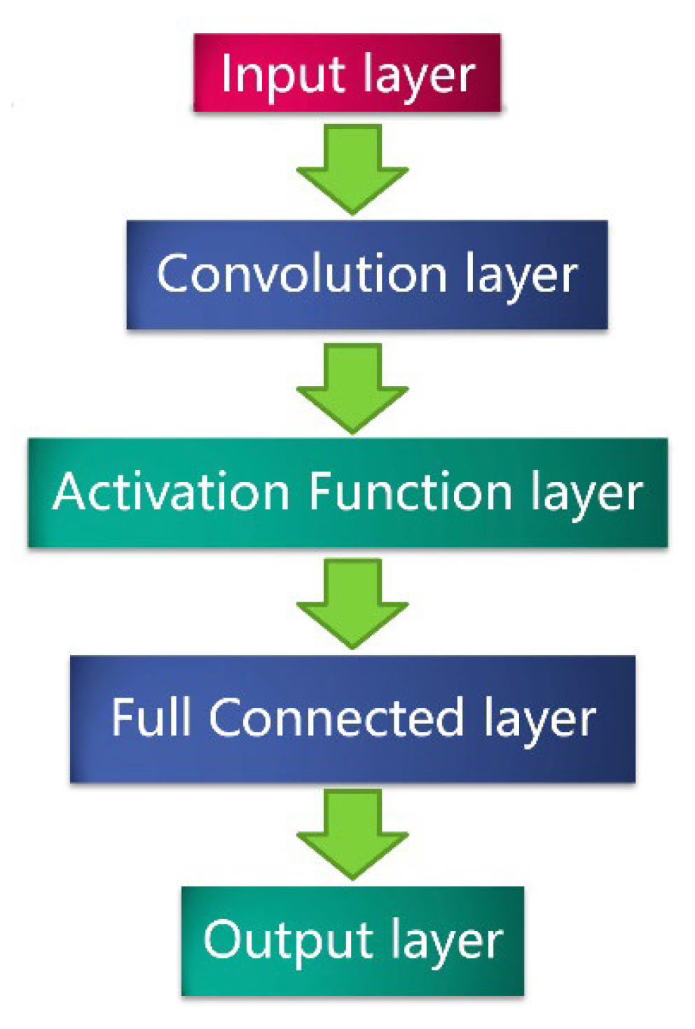
Figure 1. Topological structure of a CNN.
Remotesensing 15 03422 g001
Figure 2. Schemata of LIBS local feature extraction types using a 1D convolutional kernel function.
Remotesensing 15 03422 g002
Figure 3. Flowchart of the ECNN-based LIBS modeling framework.
Remotesensing 15 03422 g003
Figure 4. Histograms of the bootstrap sampling dataset (Si element data).
Remotesensing 15 03422 g004
Figure 5. Correspondence between the Al-relevant characteristic lines in the original LIBS data and the abstract features extracted using the CNN model.
Remotesensing 15 03422 g005
Figure 6. Features extracted by the CNN model.
Remotesensing 15 03422 g006
Figure 7. CNN-learned kernels for the LIBS dataset: (a) kernel size = 20; (b) kernel size = 50; (c) kernel size = 100.
Remotesensing 15 03422 g007
Table 1. Statistical results of element concentrations in LIBS data.
ElementSetNo. of SamplesConcentration, wt%
RangeMean ± STD 1
Original calibration dataset
SiCalibration2008.70–75.4149.46 ± 14.84
Prediction4030.90–75.4154.20 ± 13.35
AlCalibration2000.17–23.7111.56 ± 5.95
Prediction400.17–23.7110.93 ± 5.11
KCalibration2000.03–5.601.33 ± 1.37
Prediction400.05–5.431.56 ± 1.63
Expanded calibration dataset
SiCalibration14350.21–84.9055.99 ± 14.38
Prediction2870.21–84.6356.35 ± 13.65
AlCalibration14350.01–38.7915.48 ± 5.84
Prediction2870.01–38.7916.43 ± 5.91
KCalibration14350.002–12.052.51 ± 1.89
Prediction2870.002–12.052.22 ± 1.89
1 STD = standard deviation.
Table 2. Comparison of the prediction ability of the ECNN model and traditional methods.
ElementModelCalibrationPrediction
Rc2RMSECVRp2RMSEP
Original calibration dataset
SiPLS0.97872.16140.95542.9609
ELM0.8376 ± 0.04875.9013 ± 0.88210.7601 ± 0.03606.9684 ± 0.5136
CNN0.9789 ± 0.00712.2148 ± 0.31840.9724 ± 0.01732.2099 ± 0.6013
ECNN10.9899 ± 0.00341.5561 ± 0.28470.9848 ± 0.00311.6728 ± 0.1759
C-QuEST0.96952.58460.92873.7354
AlPLS0.98370.75790.95401.1499
ELM0.8795 ± 0.02282.0529 ± 0.19090.7614 ± 0.03842.5271 ± 0.2042
CNN0.9869 ± 0.00590.6983 ± 0.12350.9768 ± 0.01260.8326 ± 0.1841
ECNN10.9927 ± 0.00200.5799 ± 0.04310.9868 ± 0.00150.6785 ± 0.0898
C-QuEST0.95771.22200.88621.8028
KPLS0.97680.20790.96360.3280
ELM0.8272 ± 0.03290.5651 ± 0.05550.7895 ± 0.04000.7746 ± 0.0906
CNN0.9813 ± 0.00790.2134 ± 0.04110.9632 ± 0.05360.3345 ± 0.1275
ECNN10.9885 ± 0.00390.1907 ± 0.04470.9834 ± 0.00280.2545 ± 0.0374
C-QuEST0.96050.27140.87140.6057
Expanded calibration dataset
SiPLS0.88884.62000.88394.8997
ELM0.8861 ± 0.07434.6073 ± 1.40110.8751 ± 0.08314.7240 ± 1.3965
CNN0.9163 ± 0.08513.8111 ± 1.66850.9053 ± 0.09423.8803 ± 1.6132
ECNN10.9345 ± 0.06083.4640 ± 1.24080.9270 ± 0.06693.4894 ± 1.1912
ECNN20.9616 ± 0.00222.8140 ± 0.08250.9524 ± 0.00122.9782 ± 0.0398
AlPLS0.85782.20830.85722.2395
ELM0.8638 ± 0.06512.1042 ± 0.47470.8596 ± 0.07132.1729 ± 0.5160
CNN0.8787 ± 0.08431.9536 ± 0.57370.8661 ± 0.12642.0313 ± 0.7457
ECNN10.9095 ± 0.04581.7129 ± 0.39730.9065 ± 0.05071.7604 ± 0.4131
ECNN20.9498 ± 0.00361.3087 ± 0.04830.9436 ± 0.00131.4042 ± 0.0167
KPLS0.86080.70650.86140.7069
ELM0.8446 ± 0.07220.7277 ± 0.16600.8301 ± 0.06710.7669 ± 0.1480
CNN0.9034 ± 0.08160.5453 ± 0.22140.8924 ± 0.09340.5713 ± 0.2371
ECNN10.9348 ± 0.05780.4490 ± 0.17880.9271 ± 0.06710.4706 ± 0.1934
ECNN20.9687 ± 0.00110.3349 ± 0.00620.9645 ± 0.00200.3550 ± 0.0103
Table 3. Partial predicted results obtained with ECNN, CNN, PLS, and ELM.
ElementCCCT NameActualsECNN2CNNELMPLS
PredictedRERPredictedRERPredictedRERPredictedRER
SiNorite47.8847.191.42%46.692.45%46.612.63%46.243.40%
Picrite43.5944.081.14%42.053.50%41.285.27%40.347.42%
Shergottite48.4248.300.23%46.633.69%45.705.60%45.176.55%
NAU2-LO-S43.7843.700.17%45.022.85%47.007.37%48.2310.17%
NAU2-MED-S37.4838.542.83%40.317.54%33.4210.82%41.7111.29%
KGA-MED-S35.6436.993.79%38.578.23%42.4018.96%42.5719.46%
AlNorite14.6615.012.33%15.576.34%16.2210.72%12.5014.78%
Picrite12.3912.863.81%14.0213.12%15.3223.62%15.5225.25%
Shergottite10.8311.506.16%12.3013.77%12.3514.07%12.4815.27%
NAU2-LO-S7.637.690.80%7.832.63%7.067.34%6.8510.10%
NAU2-MED-S5.725.954.12%6.7117.36%7.0523.33%7.2927.54%
KGA-MED-S23.7121.499.39%27.0213.94%28.7721.37%29.0622.56%
KNorite0.060.0565.73%0.0549.00%0.05113.67%0.05311.63%
Picrite0.100.1099.56%0.11111.76%0.073226.80%0.12929.66%
Shergottite0.110.1144.38%0.1036.31%0.14329.97%0.1009.12%
NAU2-LO-S0.400.46115.48%0.49122.77%0.58947.41%0.52431.17%
NAU2-MED-S0.290.3127.85%0.16941.62%0.14151.21%0.14350.49%
KGA-MED-S0.260.2641.63%0.2766.24%0.28710.65%0.28610.31%
Disclaimer/Publisher’s Note: The statements, opinions and data contained in all publications are solely those of the individual author(s) and contributor(s) and not of MDPI and/or the editor(s). MDPI and/or the editor(s) disclaim responsibility for any injury to people or property resulting from any ideas, methods, instructions or products referred to in the content.