Article

Climatology of Cloud Base Height Retrieved from Long-Term Geostationary Satellite Observations

1
College of Meteorology and Oceanography, National University of Defense Technology, Changsha 410073, China
2
Key Laboratory for Atmosphere and Global Environment Observation, Chinese Academy of Sciences, Beijing 100029, China
*
Author to whom correspondence should be addressed.
These authors contributed equally to this work.
Remote Sens. 2023, 15(13), 3424; https://doi.org/10.3390/rs15133424
Submission received: 29 May 2023 / Revised: 29 June 2023 / Accepted: 3 July 2023 / Published: 6 July 2023
(This article belongs to the Section Environmental Remote Sensing)

Abstract

:
Cloud base height (CBH) is crucial for parameterizing the cloud vertical structure (CVS), but knowledge concerning the temporal and spatial distribution of CBH is still poor owing to the lack of large-scale and continuous CBH observations. Taking advantage of high temporal and spatial resolution observations from the Advanced Himawari Imager (AHI) on board the geostationary Himawari-8 satellite, this study investigated the climatology of CBH by applying a novel CBH retrieval algorithm to AHI observations. We first evaluated the accuracy of the AHI-derived CBH retrievals using the active measurements of CVS from the CloudSat and CALIPSO satellites, and the results indicated that our CBH retrievals for single-layer clouds perform well, with a mean bias of 0.3 ± 1.9 km. Therefore, the CBH climatology was compiled based on AHI-derived CBH retrievals for single-layer clouds for the time period between September 2015 and August 2018. Overall, the distribution of CBH is tightly associated with cloud phase, cloud type, and cloud top height and also exhibits significant geographical distribution and temporal variation. Clouds at low latitudes are generally higher than those at middle and high latitudes, with CBHs peaking in summer and lowest in winter. In addition, the surface type affects the distribution of CBH. The proportion of low clouds over the ocean is larger than that over the land, while high cloud occurs most frequently over the coastal area. Due to periodic changes in environmental conditions, cloud types also undergo significant diurnal changes, resulting in periodic changes in the vertical structure of clouds.

1. Introduction

Clouds cover over 60% of the Earth’s surface and have a significant impact on the energy budget, water cycle, and weather evolution through complex atmospheric chemical and physical processes [1,2]. Based on cloud observations and simulations, previous studies have demonstrated that many cloud effects, such as cloud–radiation, cloud–aerosol, and cloud–precipitation interactions, are highly related to the vertical distribution of clouds [3,4]. Therefore, as an important macrophysical property to describe the vertical distribution of clouds, cloud base height (CBH) is crucial for understanding the role of clouds in weather and climate [5,6]. In addition, accurate CBH information has practical value in the aviation community because it can help to identify potential aircraft icing and plan a safety route.
There have been extensive studies on the relationship between CBH and cloud effects, particularly for the cloud radiative effect (CRE). For example, Randall et al. [7] indicated that a 4% increase in the global coverage of marine stratocumulus clouds (most of them have CBHs smaller than 1 km) would result in 2–3 K decrease in global temperature that could offset the predicted warming effect caused by a doubling of atmospheric carbon dioxide. McFarlane et al. [8] indicated that low clouds contributed 71–75% of the surface shortwave CRE and 66–74% of the surface longwave CRE at three tropical western Pacific Ocean sites. Viúdez-Mora et al. [9] reported that the average CRF at a midlatitude site for summer and winter decreased with CBH at a rate of −5 and −4 W m−2 km−1, respectively. Based on global cloud observations and simulations, Zelinka et al. [4] indicated that high, thin clouds and low, opaque clouds have different effects on cloud feedback and may compete with each other as the main driver of overall cloud feedback. However, owing to different cloud parameterization schemes, there are considerable differences in simulating CRF from different GCMs. As a result, large intermodel differences in modeling climate change still exist [10]. To reduce the uncertainties in cloud simulations from different general circulation models (GCMs), there is a need for long-term and continuous and large-scale cloud observations to improve cloud parameterization schemes.
The most reliable CBH observations are typically derived from ground-based instruments, such as lidar ceilometers and millimeter-wave radars [11,12]. However, the CBH observations from surface sites have very limited coverage; thus they are mainly utilized by airports for ensuring aviation safety and are not suitable for analysis of weather or climate. The CloudSat and the Cloud-Aerosol Lidar and Infrared Pathfinder Satellite Observations (CALIPSO) satellites are powerful tools for global remote sensing of cloud vertical structures and cloud microphysical properties from space [13,14]. While CloudSat and CALIPSO are capable of measuring CBH globally, they only cover the nadir pixels and cannot be used for continuously monitoring weather systems such as tropical cyclones due to their polar orbits. In contrast, passive radiometers on board geostationary satellites, such as the Advanced Himawari Imager (AHI) on board Himawari-8 and the Advanced Geosynchronous Radiation Imager (AGRI) on board FY-4A, can continuously observe clouds over much larger coverages, and their visible and infrared radiance measurements have been successfully used to retrieve cloud top height (CTH) [15,16,17,18]. However, the visible and infrared radiance measurements contain limited information concerning cloud vertical structures due to penetration limitation, resulting in difficulty in the retrieval of CBH [19,20]. To overcome the limitations of passive radiometers, several methods have been developed to extrapolate the CBH measurements from CloudSat to a wider coverage of the Moderate Resolution Imaging Spectroradiometer (MODIS) [21,22,23]. Besides, other studies attempted to estimate CBH independently from passive radiometer measurements. For example, Hutchison et al. [24] utilized six cloud-type-determined empirical cloud water contents (CWC) to bridge cloud water path (CWP) and cloud geometric thickness (CGT); subsequently, the CBH retrievals can be obtained by subtracting the estimated CGTs from conventional cloud top height (CTH) retrievals. Noh et al. [23] related CBH to CWP via a CTH-dependent piecewise linear fitting method, and achieved higher retrieval accuracy in the Visible Infrared Imaging Radiometer Suite (VIIRS) on board the Suomi National Polar-Orbiting Partnership (SNPP) satellite. Moreover, machine learning (ML) techniques have been introduced to estimate CBH from passive radiometers. Lin et al. [25] presented an ML-based method to estimate daytime single-layer CBH based on Geostationary Operational Environmental Satellite-R Series (GOES-16) Advanced Baseline Imager (ABI) level 1b data and the European Centre for Medium-Range Weather Forecasts’ (ECMWF) fifth-generation reanalysis (ERA5) data, and can provide CBH estimates with high spatial (2 km) and temporal (10 min) resolution.
Previous studies have used CBH measurements derived from ground-based and satellite-based radars to investigate the climatology of CBH, which increased our knowledge on the CBH distribution and the relationship between CBH and CRE [12]. However, the limited observational coverage of radars prevents broader analysis, such as cloud climatology and the continuous monitor of cloud vertical structures in mesoscale weathers systems. An analysis based on long-term and large-scale CBH data derived from geostationary satellite observations would be useful for conducting these tasks. In particular, our previous study developed a novel CBH retrieval algorithm for passive radiometers [26], providing an opportunity to analyze the climatology of CBH.
In this study, we applied the CBH retrieval algorithm developed by [26] to the geostationary Himawari-8 satellite observations to produce a continuous and large-scale CBH dataset, which will be utilized to analyze the CBH climatology related to cloud properties, seasons, and geolocations. The remainder of this paper is organized as follows: Section 2 introduces the data and the CBH retrieval method. Section 3 illustrates the CBH climatology. Finally, Section 4 concludes the paper.

2. Data and Methodology

2.1. Data

The Himawari-8 satellite is a new-generation geostationary satellite that has been operated by Japan Meteorological Agency since 7 July 2015 [27,28,29]. The AHI on board Himawari-8 has 16 spectral channels, including 4 visible and near-infrared channels (0.47–0.86 μm), 2 shortwave infrared channels (1.6–2.3 μm), 1 medium-wave infrared channel (3.9 μm), and 9 longwave infrared channels (5–14 μm). The AHI performs full-disk observation every 10 min with high spatial resolution (~5 km) over a wide region generally defined as 80°E to 160°W and 60°S to 60°N. The AHI measurements have been used to produce various cloud, atmospheric, and land property products. In this study, the AHI level 2 (L2) cloud property (CLP) product provides cloud mask, cloud phase, cloud optical properties, and cloud top properties that are necessary input variables for the estimate of CBH [17]. Besides, the AHI level 1b (L1b) product is utilized for multilayer cloud detection, which will be used for data quality control.
To examine the performance of the CBH retrievals from the AHI, we consider the active satellite measurements, i.e., spaceborne radar and lidar data. The cloud profiling radar (CPR) on board CloudSat is well skilled to detect the vertical structures of relatively thick clouds, except for precipitation clouds [30]. In contrast, the Cloud-Aerosol Lidar with Orthogonal Polarization (CALIOP) on board CALIPSO has advantages on detecting optically thin clouds [14]. CPR and CALIOP combined products (e.g., 2B-CLDCLASS-LIDAR) combine these advantages to provide more accurate CBHs [30]. Therefore, the 2B-CLDCLASS-LIDAR products are used to evaluate our AHI CBH dataset. The satellite products and variables are summarized in Table 1.

2.2. CBH Estimation Method

Direct retrieval of CBH is theoretically difficult for passive satellite radiometers, such as the AHI, because satellite radiometric measurements from cloudy pixels are mainly determined by cloud top properties. Hence, most existing methods first estimate CGT using conventional CWP retrievals, and then calculate CBH as the difference between the CGT retrievals and existing CTH retrievals. Recently, Tan et al. [26] developed a method to retrieve CBH from passive radiometers, utilizing an improved characterization for mutable cloud water contents (CWCs). This was achieved by introducing a variable named effective CWC (ECWC) to represent the vertically varying CWC and subsequently constructing a systematic ECWC lookup table (LUT) based on collocated active and passive satellite observations. With the developed ECWC LUT, we can convert the existing CWP (kg/m2) to CGT (km), and calculated CBH by subtracting the CGT retrievals from conventional CTH retrievals. The algorithm is applicable for all cloudy pixels having valid CTH and CWP inputs, and the algorithm has high computer efficiency because no radiative transfer model is needed in the calculation. Because the Himawari-8 satellite currently provides only a daytime CWP product derived from visible and near-infrared spectral measurements [17], the retrieval of CBH in this study can be only conducted for daytime observations. While this limitation prevents the analysis for nighttime CBHs, this study is still meaningful and indispensable for understanding the climatology of CBH, because our geostationary satellite-based CBH retrievals have distinct advantages on observational coverages and observational frequencies compared with ground-based or spaceborne radar measurements.
Three-year AHI data from September 2015 to August 2018 were used to produce the analysis dataset. Besides our CBH retrievals, the dataset also includes the existing cloud top and cloud optical properties in the AHI products provided by the Japan Aerospace Exploration Agency (JAXA) P-Tree system (ftp.ptree.jaxa.jp). The analysis dataset has a temporal resolution of 10 min and a spatial resolution of 0.05° latitude/longitude within the observational coverage of the AHI.

2.3. Data Quality Control

Before the analysis, the retrieved CBHs were evaluated using the active measurements derived from 2B-CLDCLASS-LIDAR. Figure 1 shows an example of the AHI CBH retrievals on 5 October 2017 at UTC 05:20. While CPR and CALIOP can detect the vertical structures of clouds accurately for nadir pixels indicated by a black line in Figure 1a, our CBH retrievals based on AHI measurements are available over much wider areas. Figure 1b shows a cross-section comparison between our CBH retrievals and those from 2B-CLDCLASS-LIDAR, corresponding to the along-track pixels marked by black lines in Figure 1a. One can see that the CBH retrievals are mostly close to those determined by 2B-CLDCLASS-LIDAR. There are significant CBH biases caused by multilayer clouds in regions near 53°S. This is because the AHI cloud property products are produced on the single-layer cloud assumption and may be largely biased in multilayer cloud cases [31,32,33]. Clearly, the errors inherited from upstream cloud property products would affect the CBH retrievals. However, not all multilayer clouds would lead to significant errors. If upper clouds were optically thin, e.g., multilayer clouds in regions between 52°S to 48°S in Figure 1a, they may be overlooked due to the limited spectral sensitivity of the AHI; thus their influence on CBH retrievals may be little.
Figure 2 presents a statistical evaluation based on spatiotemporally collocated AHI-CPR-CALIOP data from September 2015 to August 2018. The CBH differences between AHI and CPR-CALIOP are calculated for single-layer clouds and multilayer clouds, respectively. Table 2 lists the error statistics of the differences between AHI and CPR-CALIOP. The results indicate that our CBH retrieval algorithm is particularly efficient for single-layer clouds, with a mean bias of 0.2 ± 1.9 km. However, owing to the aforementioned limitations, multilayer clouds can lead to significant underestimation in the retrievals of CBH with a mean bias of −3.2 ± 3.7 km. Therefore, multilayer clouds, which account for approximately 26% of all cloudy pixels in our dataset, are excluded from the CBH dataset for valid analysis. Here, multilayer clouds are detected via the algorithm offered by [34], which is well skilled to label multilayer cloud pixels with large cloud property retrieval errors. Besides multilayer clouds, previous studies have reported that precipitation clouds would introduce large uncertainties in cloud property retrievals. Thus, only single-layer nonprecipitation clouds are included in our final CBH dataset for analysis.

3. Climatology of CBH

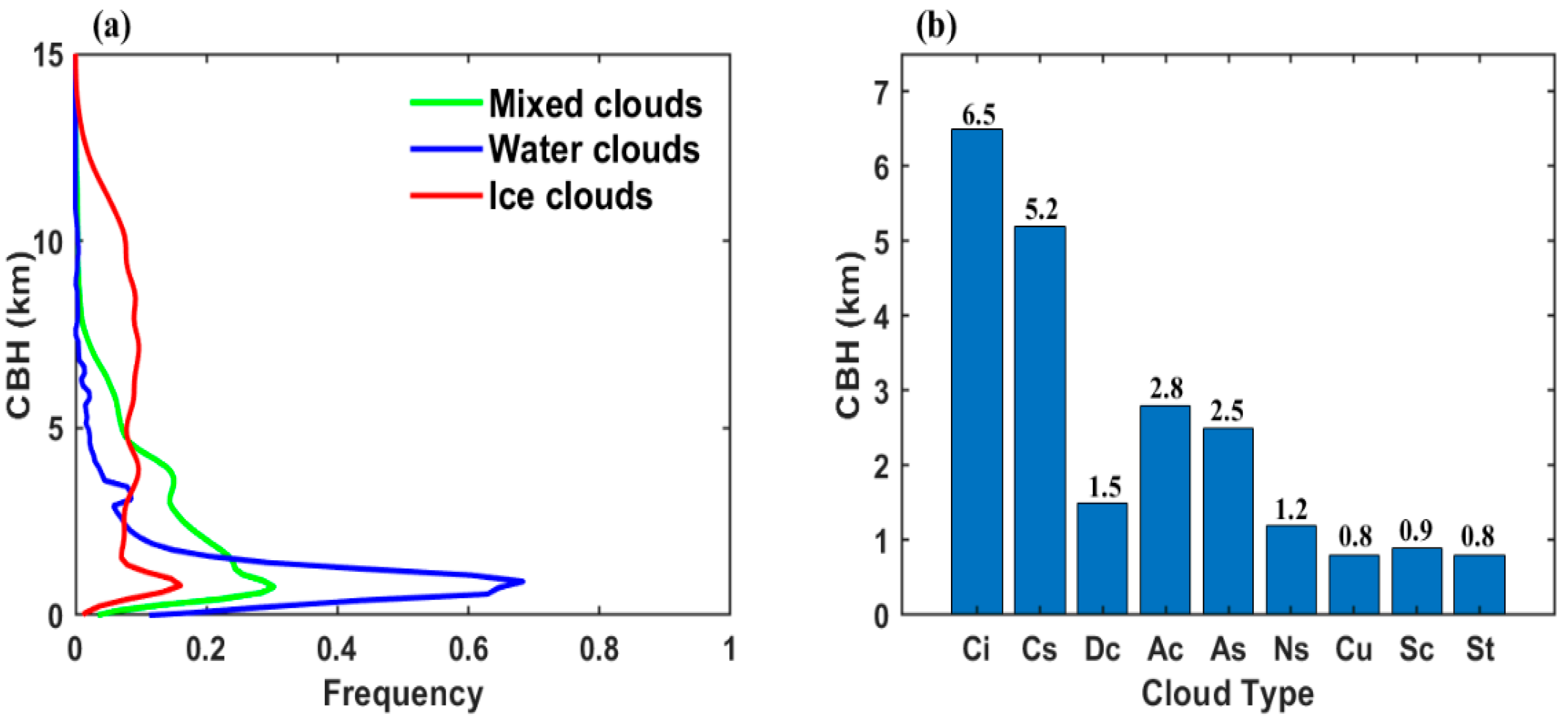
3.1. Relationship between CBH and Cloud Properties

The analysis of CBH characteristics is first conducted for different cloud thermodynamic phases and cloud types. Cloud phase denotes the phase of cloud drop at the cloud top, defined as ice, water, and mix. Based on multiband visible and infrared measurements (e.g., 8.6 and 11.2 μm) and various empirical lookup tables of thresholds developed for different geometric conditions and surface types, cloud phases could be reasonably inferred by the AHI. For cloud type determination, current AHI products follow the definition of the International Satellite Cloud Climatology Project (ISCCP). Specifically, clouds are classified into nine types based on cloud top pressure (CTP) and cloud optical thickness (COT), including cirrus (Ci), cirrostratus (Cs), deep convection (DC), altocumulus (Ac), altostratus (As), nimbostratus (Ns), cumulus (Cu), stratocumulus (Sc), and stratus (St). Both cloud phase and cloud type are fundamental for the retrieval of cloud top properties and cloud optical properties. Therefore, studying the relationship between CBH distribution and cloud phase/type would be informative for improving the satellite-based retrieval of cloud properties.
Figure 3 shows the frequency distribution of CBH for different cloud phases and the mean CBH for different cloud types. It should be noted that the results cover clouds from different surface types, seasons, and atmospheric conditions. As shown in Figure 3a, the CBHs of water clouds are mostly smaller than 1.5 km, indicating that the bottoms of liquid water clouds are typically close to the surface. These low-level clouds are mainly distributed over oceans, and have significant influence on global climate change due to their strong reflectance for incoming solar radiation and strong emission of infrared radiation [35]. In addition, low clouds are also correlated to cloud–aerosol–precipitation interaction, and its properties are important for atmospheric pollution and weather modification studies [36]. For mix clouds, approximately 40% of the CBHs are smaller than 1.5 km, and the remaining are distributed from 1.5 to 8 km. As expected, most ice clouds occur in the middle and high levels in the troposphere. Ice clouds are one of several common aviation threats because the low temperatures and high humidity within the cloud may cause aircraft to freeze. Since geostationary satellites can continuously observe clouds over most of the globe (except for polar regions), the satellite-retrieved CBHs may be valuable for the aviation community.
Figure 3b shows the mean CBH for nine AHI-determined cloud types. Ci has the largest CBH of 6.5 km, followed by Cs at 5.2 km. DC clouds are recognized as high-level clouds because of their large CTH. However, due to strong convection, DC clouds are typically very thick, and their cloud base is close to the surface. For midlevel clouds, the mean CBHs of Ac and As clouds are relatively high at 2.8 and 2.5 km, respectively. By contrast, Ns appears to be closer to the surface. The low-level clouds, including Cu, Sc, and St, have similar mean CBHs at approximately 0.8 km. The CBH information may contribute to better estimate the CRE as previous studies on CRE have mainly focused on cloud top properties and cloud microphysical properties. Moreover, the current AHI cloud classification method only utilizes CTP and COT, ignoring vertical cloud structures. Therefore, adding CBH information could improve the identification of cloud types, which is a topic for future research.
Vertical cloud structures are also important cloud properties, as many cloud-related effects vary widely with the cloud vertical distribution. Here, we analyze the CBH distribution related to CTH and CGT. Based on the AHI CBH dataset, the sample number of each 1 × 1 km CBH-CTH and CBH-CGT box was calculated, respectively. In the analysis, CTH, CBH, and CGT range from 0 to 16 km. As shown in Figure 4a, CBH has clear dependency on CTH. When the CTHs are smaller than 3 km, the CBHs are mostly below 1 km. If the CTH is between 4 and 12 km, the most frequent CBHs are generally approximately 3 km smaller than the corresponding CTHs, indicating that most CGTs are approximately 3 km. If the CTH exceeds 12 km, a large proportion of CBH is relatively small, meaning that these clouds are thick. Figure 4b illustrates the relationship between CBH and CGT. Consistent with the findings in Figure 4a, most clouds have CGTs between 0 and 4 km; the occurrence frequency of CGT peaks at approximately 3 km. When CGT is larger than 4 km, the occurrence frequency of clouds decreases with increasing CGT. In addition, when the CGTs are smaller than 1 km, the CBHs are also mostly smaller than 1 km. These low and thin clouds are mainly marine SC clouds, which cover over 20% of the low-latitude oceans and are an important modulator of global radiance balance. As the CGT increases, DC and NS clouds may dominate because the strong convection generally results in thick clouds.
In summary, the CBH distribution is highly sensitive to cloud properties. Not only cloud type and cloud phase but also CTH and CGT significantly affect the distribution of CBH. These analyses are similar to previous studies based on ground-based or spaceborne radar measurements, but our results are derived from a huge sample covering different environmental conditions and may contribute to improving the cloud parameterization models.

3.2. Geographical Distribution and Seasonal Variation of CBH

The CBH distribution associated with cloud properties was investigated by the figures above. To gain a better understanding of the environmental conditions’ impact on CBH, we further investigated the geographical distribution and seasonal variation of CBH. In particular, the wide observational coverage of geostationary satellites allows us to study the regional characteristics of cloud properties, which may be important for the improvement regional climate models.
Figure 5 shows the mean CBHs within the AHI observational coverage for different seasons. The geographical distribution of CBH is first discussed. As shown in Figure 5a, the CBH distribution has obvious latitudinal variation, as the mean CBH in the tropical regions is larger than those in midlatitude regions. This is highly related to the distribution of cloud types, as previous studies have reported that the tropical regions are mostly covered by Ci/Cs and the midlatitude regions have a larger percentage of midlevel and low-level clouds (e.g., As, Ac, and Sc). Within our study area, the largest mean CBH (>6 km) generally occurs in the Marine Continent, and the smallest mean CBHs (<1 km) are mainly found in the midlatitude seas of the southern hemisphere. Moreover, the mean CBH may be correlated to the surface types. For example, the mean CBHs for clouds over midlatitude ocean are generally smaller than 2 km, while those for clouds over midlatitude land are mostly larger than 3 km. As a result, the mean CBH in the northern hemisphere tends to be generally larger than that in the southern hemisphere. An interesting finding is that the mean CBH typically reaches regional maximums in coastal regions (defined as the ocean within 100 km from the coastline), such as the southeastern coast of New Zealand and the southwestern cost of Indonesia. Our understanding is that larger CBHs in coastal areas may be caused by sea–land winds. Due to the difference in thermal properties between land and sea, the air temperature near the ground on land in the daytime is generally higher than that over the ocean, and the pressure is lower than that over the ocean. Thus, lower-level air may blow from the sea to the land, while upper-level air flows from the land to the ocean. The circulation caused by the sea–land wind could lead to more high clouds over the ocean and more low clouds to gather over the land. To better illustrate the differences caused by the surface, Figure 6 shows the CBH distributions over land, ocean, and coastal areas, respectively. The most common CBH for clouds over land is approximately 3 km, and the mean and median CBH of which are 3.9 and 3.3 km, respectively. In land areas, the proportion of clouds with a CBH between 0 and 3 km is about 50% and becomes very small when the CBH is greater than 8 km. In contrast, there were more low clouds over the ocean, and the proportion of clouds with a CBH between 0 and 3 km increased to about 70%. Moreover, oceanic clouds with a CBH between 4 and 7 km are less frequent than land clouds, and the mean (2.8 km) of oceanic CBHs is smaller than that of land clouds. For clouds in coastal areas, the proportion of CBH larger than 7 km is higher than that for land and ocean, leading to the largest mean CBH of 4.4 km.
Figure 5b–d show the geographical distribution of the mean CBH in different seasons, i.e., March–April–May (MAM), June–July–August (JJA), September–October–November (SON), and December–January–February (DJF). To better illustrate the seasonal variation of vertical cloud structures, the mean CTH, CBH, and CGT for different seasons and latitudes are also presented in Table 3. During MAM, the distribution along the latitude of the mean CBH is relatively symmetrical, and tropical clouds tend to be higher and thicker than midlatitude clouds. The mean CTH, CBH, and CGT in MAM are approximately 6.8, 3.8, and 3.0 km in the tropics, respectively, while those for midlatitude clouds are 4.1, 1.8, and 2.3 km. During JJA, the peak of the mean CBH moves north to about 15°N, and the mean CBH in most of the northern hemisphere areas (e.g., South China Sea) increases. As a result, the mean CTH, CBH, and CGT of midlatitude clouds in the northern hemisphere increase to 5.75, 2.71, and 3.03 km, respectively. Moreover, the mean CTH, CBH, and CGT become smaller in the southern hemisphere, indicating that clouds are typically higher, thicker in summer and lower, thinner in winter. The CBH distribution in SON is similar to that in MAM, but the mean CTH, CBH, and CGT in the northern hemisphere are larger in SON than in MAM. During DJF, the mean CTH, CBH, and CGT in the southern hemisphere increase, and those in the northern hemisphere decrease. However, the seasonal variation of the mean CBH in the southern hemisphere (from 1.47 to 2.04 km) is less significant than that in the northern hemisphere (from 1.48 to 2.71 km), possibly caused by the smaller proportion of landmass in the southern hemisphere. In addition, the seasonal and latitudinal variations for both CTH and CBH appear to be more intensive than that for CGT, indicating that seasons and geolocations may have more impacts on the vertical locations than the thickness of clouds.
The vertical distribution of clouds is important for many cloud-related studies, and has been found to significantly vary with environmental conditions, e.g., seasons and geolocations. To better understand the relationship between cloud vertical structures and geolocations, we divided the cloud pixels into three categories based on CBH (i.e., 0 < CBH < 2 km; 2 km < CBH < 6 km; 6 km < CBH) and, subsequently, calculated the occurrence frequency of each CBH category, respectively. As shown in Figure 7a, clouds occur very frequently over the ocean, as the mean cloud cover is mostly larger than 0.7. By contrast, the mean cloud cover varies widely over land. While the mean cloud covers over many land areas (e.g., Indonesia, Japan, and southeastern China) are as large as over the ocean, it may be quite small over some inland areas, especially over deserts.
The occurrence frequency of clouds with different CBH ranges is shown in Figure 7b–d. Clouds with CBHs between 0 and 2 km are quite common over the midlatitude ocean in both hemispheres, but their frequency becomes relatively small in most land areas. For clouds with CBHs between 2 and 6 km, the variation of their geographical distribution is less significant, as the occurrence frequency of most of these clouds is approximately 0.1. Clouds with CBH larger than 6 km occur most frequently over the ocean in the tropics. Additionally, since our CBH retrievals are defined as height above sea level, the retrieved CBHs over the plateau are generally high. For instance, there is a relatively large percentage of high clouds in the Tibet region. To conclude, Figure 7 indicates that the geographical distribution of clouds is tightly related to vertical cloud structures. For example, clouds in the midlatitude ocean are mainly contributed by low clouds, and tropical clouds are mainly contributed by high clouds.

3.3. Diurnal Variation of CBH

Due to the cyclical changes in environmental conditions, the macro- and microphysical properties of clouds typically have obvious diurnal variations. While the diurnal characteristics of cloud systems are important for many atmospheric scientific studies, continuous observation of regional cloud properties remains a challenging task. In this section, the cloud property retrievals derived from three years geostationary satellite observations were analyzed to investigate the diurnal variation of cloud vertical structures. The analysis was conducted for clouds over the New Guinea Island and its surrounding oceanic areas (from 120°E to 160°E and from 10°N to 10°S). Considering the obvious differences in CBH distribution between land, ocean, and coastal areas, the analysis is separately performed for clouds over different surface types.
Figure 8 shows the temporal variation of cloud types and cloud vertical structures (i.e., CTH, CBH, and CGT) from local time 07:00 to 18:00. To better illustrate the relationship between cloud type and cloud vertical structures, the nine AHI-determined cloud types are further classified into four categories: (1) Ci and Cs; (2) As and Ac; (3) St, Sc, and Cu; and (4) Dc and Ns. The cloud fractions of these four cloud categories are calculated and hourly averaged for clouds over land, ocean, and coastal areas. In addition, the mean CTH, CBH, and CGT of all cloud types are calculated and hourly averaged, as displayed in the right panels of Figure 8.
Previous studies have indicated that the development of clouds is significantly influenced by convection activities [37], which generally strengthens in the afternoon over land and early morning over ocean in the tropics. As shown in Figure 8a, clouds over land are dominated by Ci and Cs in most of daytime, accounting for approximately half of the cloudy pixels. Please note that if there are low clouds below the high clouds, only the high clouds are shown here, because it is very difficult for passive radiometers to detect the low clouds in multilayer cloud cases. On land, the number of convective clouds is minimum between local time 10:00 and 12:00 and increases rapidly after 12:00. After the deep convective cloud ratio increased, the cirrus/cirrostratus cloud ratio also gradually increased, which may be related to the periphery of the deep convective cloud. Previous studies have shown that the deep convective diffusion of cirrus is a characteristic of a deep convective system at the maturity and dissipation stage. Cirrus cloud coverage grows during the mature phase of the deep convective system and gradually weakens 1–2 h after the onset of surface convective rainfall. At the same time, the ratio of middle cloud to low cloud drops rapidly after 12:00. Due to changes in cloud types, the vertical structure of clouds also changes significantly. As shown in Figure 8b, with the increase in convective cloud proportion, both the height of the cloud top and the geometric thickness of the cloud increase rapidly, indicating that the cloud becomes taller and thicker. For clouds over the ocean, the diurnal variation in convective activity appears to be less intense than over land, and the time periods of convective intensification are different from those over land. In Figure 8e, the proportion of deep convective clouds is about 16%, with little fluctuation, but the proportion is higher between local standard time (LST) 08:00 and 12:00 than after LST 12:00. Except for deep convective clouds, the diurnal variation of other types of clouds in the marine area is not as obvious as that in the land area. The proportion of high-, middle-, and low-level clouds is about 58%, 17%, and 8%. Accordingly, the vertical structure of clouds in the ocean region is relatively flat. The height of the cloud top and the height of the cloud base are the minimum before LST 09:00, and then two maximum values appear at LST 10:00 and 15:00. The variation characteristics of coastal areas are very similar to those of marine areas, but the proportion of high clouds is slightly higher. These results indicate that periodic changes in the environment will lead to significant diurnal variations in cloud characteristics. For example, the warming of the land area at noon increases convective activity so that the ratio of deep to convective clouds generally increases at LST 12:00, resulting in a corresponding increase in cloud height and thickness. By analyzing and summarizing the changing laws of these cloud characteristics, we will deepen our understanding of clouds and provide important observational evidence for the development and improvement of cloud parameterization schemes in weather and climate models [38].

4. Conclusions

Taking advantage of high spatiotemporal resolution observations of the geostationary Himawari-8 satellite, this study produced a climatology of CBH by applying an advanced algorithm for retrieving CBH to the radiometric observations of AHI. The relationship between CBH and other cloud properties has been investigated, as well as the spatial and temporal distribution of CBH. The investigation covers a large area from 60°N to 60°S and from 80°E to 160°W and covers three years observations from 2015 to 2018. Compared with previous studies based on ground-based or satellite radar measurements, our statistics derived from large-scale and continuous observations of a geostationary satellite contribute to a better understanding of cloud climatology.
The results indicate that the distribution of CBH is tightly associated with cloud phase, cloud type, and cloud top height. Most liquid water clouds have CBHs of less than 1.5 km, while more than 60% of ice clouds have CBHs of more than 5 km. For cloud types, the largest average CBH of 6.5 km is for cirrus clouds; that of altocumulus cloud is about 2.8 km; and that of stratus cloud, stratus cumulus cloud, and cumulus cloud is very similar, which is about 0.8 km. The distribution of CBH also shows significant geographical distribution and temporal variation. Clouds at low latitudes are generally higher than those at middle and high latitudes, and CBHs are typically highest in summer and lowest in winter. In addition, the surface type affects the distribution of CBH. The proportion of low clouds over the ocean is obviously larger than that over the land, while high clouds occur most frequently over the coastal area. Due to periodic changes in environmental conditions, cloud types also undergo significant diurnal changes, resulting in periodic changes in the vertical structure of clouds.
Although the CBH retrievals from passive radiometer observations may be not as accurate as active radar measurements, this study provides a viable approach to investigate the spatial and temporal distribution of CBH via geostationary satellite observations. Such information will contribute to better quantifying the cloud radiative effects highly correlated to cloud vertical structures. However, the climatology of CBH in this study was only derived from daytime CBH retrievals because the CBH retrieval algorithm requires cloud optical thickness as input. Therefore, future work will aim to obtain nighttime CBH information from geostationary satellite observations [39], which will be of significance for improving our understanding of cloud climatology.

Author Contributions

Conceptualization, Z.T. and X.Z.; methodology, Z.T.; software, S.H.; validation, Z.T., W.A. and X.Z.; investigation, S.M.; resources, S.H.; data curation, X.W.; writing—original draft preparation, Z.T. and X.Z.; writing—review and editing, S.M.; visualization, W.A. and L.W.; supervision, S.H.; project administration, X.W.; funding acquisition, X.W. All authors have read and agreed to the published version of the manuscript.

Funding

This research is supported by the Provincial Natural Science Foundation of Hunan (2023JJ40665), the Strategic Priority Research Program of the Chinese Academy of Sciences (grant no. XDA15021000), and the National Natural Science Foundation of China (grants no. 41705007).

Data Availability Statement

The AHI data are available at https://www.eorc.jaxa.jp/ptree (accessed on 4 July 2015). The ERA5 data are available on the Copernicus Climate Change Service Climate Data Store (https://cds.climate.copernicus.eu (accessed on 1 January 1950)). The CPR and CALIOP data are available at https://www.cloudsat.cira.colostate.edu/data-products/2b-cldclass-lidar (accessed on 7 July 2006).

Conflicts of Interest

The authors declare no conflict of interest. The funders had no role in the design of the study; in the collection, analyses, or interpretation of data; in the writing of the manuscript; or in the decision to publish the results.

References

  1. Baker, M.B. Cloud microphysics and climate. Science 1997, 267, 1072–1078. [Google Scholar] [CrossRef]
  2. Norris, J.R.; Allen, R.J.; Evan, A.T.; Zelinka, M.D.; O’Dell, C.W.; Klein, S.A. Evidence for climate change in the satellite cloud record. Nature 2016, 536, 72–75. [Google Scholar] [CrossRef] [Green Version]
  3. Qian, Y.; Long, C.N.; Wang, H.; Comstock, J.M.; McFarlane, S.A.; Xie, S. Evaluation of cloud fraction and its radiative effect simulated by IPCC AR4 global models against ARM surface measurements. Atmos. Chem. Phys. 2012, 12, 1785–1810. [Google Scholar] [CrossRef] [Green Version]
  4. Zelinka, M.D.; Randall, D.A.; Webb, M.J.; Klein, S.A. Clearing clouds of uncertainty. Nat. Clim. Change 2017, 7, 674–678. [Google Scholar] [CrossRef]
  5. Chen, Y.; Wang, H.; Min, J.; Huang, X.; Minnis, P.; Zhang, R.; Haggerty, J.; Palikonda, R. Variational Assimilation of Cloud Liquid/Ice Water Path and Its Impact on NWP. J. Appl. Meteorol. Climatol. 2015, 54, 1809–1825. [Google Scholar] [CrossRef]
  6. Jones, T.A.; Stensrud, D.J. Assimilating Cloud Water Path as a Function of Model Cloud Microphysics in an Idealized Simulation. Mon. Wea. Rev. 2015, 143, 2052–2081. [Google Scholar] [CrossRef]
  7. Randall, D.; Coakley, J., Jr.; Fairall, C.; Kropfli, R.; Lenschow, D. Outlook for research on subtropical marine stratiform clouds. Bull. Am. Meteor. Soc. 1984, 65, 1290–1301. [Google Scholar] [CrossRef]
  8. McFarlane, S.A.; Mather, J.H.; Ackerman, T.P. Analysis of tropical radiative heating profiles: A comparison of models and measurements. J. Geophys. Res. 2007, 112, D14218. [Google Scholar] [CrossRef] [Green Version]
  9. Viúdez-Mora, A.; Costa-Surós, M.; Calbó, J.; González, J.A. Modeling Atmospheric Longwave Radiation at the Surface During Overcast Skies: The Role of Cloud Base Height. J. Geophys. Res. Atmos. 2014, 120, 199–214. [Google Scholar] [CrossRef] [Green Version]
  10. Potter, G.L.; Cess, R.D. Testing the impact of clouds on the radiation budgets of 19 atmospheric general circulation models. J. Geophys. Res. 2004, 109, D02106. [Google Scholar] [CrossRef] [Green Version]
  11. Huo, J.; Lu, D.; Duan, S.; Bi, Y.; Liu, B. Comparison of the cloud top heights retrieved from MODIS and AHI satellite data with ground-based Ka-band radar. Atmos. Meas. Tech. 2020, 13, 1–11. [Google Scholar] [CrossRef] [Green Version]
  12. Zhang, Y.; Zhang, L.; Guo, J. Climatology of cloud-base height from long-term radiosonde measurements in China. Adv. Atmos. Sci. 2018, 35, 158–168. [Google Scholar] [CrossRef]
  13. Stephens, G.L.; Vane, D.G.; Boain, R.J.; Mace, G.G.; Sassen, K. The CloudSat mission and the A-Train: A new dimension of space-based measurements of clouds and precipitation. Bull. Am. Meteorol. Soc. 2002, 83, 1771–1790. [Google Scholar] [CrossRef] [Green Version]
  14. Winker, D.M.; Vaughan, M.A.; Omar, A.; Hu, Y.; Powell, K.A.; Liu, Z.; Hunt, W.H.; Young, S.A. Overview of the CALIPSO mission and CALIOP data processing algorithms. J. Atmos. Ocean. Technol. 2009, 26, 2310–2323. [Google Scholar] [CrossRef]
  15. Menzel, W.P.; Frey, R.A.; Zhang, H.; Wylie, D.P.; Moeller, C.C.; Holz, R.; Maddux, B.; Baum, B.A.; Strabala, K.I.; Gumley, L.E. MODIS global cloud-top pressure and amount estimate: Algorithm description and results. J. Appl. Meteorol. Climatol. 2008, 47, 1175–1198. [Google Scholar] [CrossRef] [Green Version]
  16. Min, M.; Wu, C.; Li, C.; Liu, H.; Xu, N.; Wu, X.; Chen, L.; Wang, F.; Sun, F.; Qin, D.; et al. Developing the science product algorithm testbed for Chinese next-generation geostationary meteorological satellites: Fengyun-4 series. J. Meteorol. Res. 2017, 31, 708–719. [Google Scholar] [CrossRef]
  17. Iwabuchi, H.; Putri, N.S.; Saito, M.; Tokoro, Y.; Sekiguchi, M.; Yang, P.; Baum, B.A. Cloud property retrieval from multiband infrared measurements by Himawari-8. J. Meteor. Soc. Jpn. 2018, 96, 27–42. [Google Scholar] [CrossRef] [Green Version]
  18. Min, M.; Li, J.; Wang, F.; Liu, Z.; Menzel, W.P. Retrieval of cloud top properties from advanced geostationary satellite imager measurements based on machine learning algorithms. Remote Sens. Environ. 2020, 239, 111616. [Google Scholar] [CrossRef]
  19. Hutchison, K.D. The retrieval of cloud base heights from MODIS and three-dimensional cloud fields from NASA’s EOS Aqua mission. Int. J. Remote Sens. 2002, 23, 5249–5265. [Google Scholar] [CrossRef]
  20. Seaman, C.J.; Noh, Y.-J.; Miller, S.D.; Heidinger, A.K.; Lindsey, D.T. Cloud base height estimate from VIIRS. Part I: Operational algorithm validation against CloudSat. J. Atmos. Ocean. Technol. 2017, 34, 567–583. [Google Scholar] [CrossRef] [Green Version]
  21. Barker, H.W.; Jerg, M.P.; Wehr, T.; Kato, S.; Donovan, D.P.; Hogan, R.J. A 3D cloud-construction algorithm for the Earth CARE satellite mission. Quart. J. Roy. Meteor. Soc. 2011, 137, 1042–1058. [Google Scholar] [CrossRef] [Green Version]
  22. Miller, S.D.; Forsythe, J.M.; Partain, P.T.; Haynes, J.M.; Bankert, R.L.; Sengupta, M.; Mitrescu, C.; Hawkins, J.D.; Haar, T.H.V. Estimating three-dimensional cloud structure via statistically blended satellite measurements. J. Appl. Meteorol. Climatol. 2014, 53, 437–455. [Google Scholar] [CrossRef] [Green Version]
  23. Noh, Y.J.; Forsythe, J.M.; Miller, S.D.; Seaman, C.J.; Li, Y.; Heidinger, A.K.; Lindsey, D.T.; Rogers, M.A.; Partain, P.T. Cloud-base height estimation from VIIRS. Part Ⅱ: A statistical algorithm based on a-train satellite data. J. Atmos. Ocean. Technol. 2017, 34, 585–598. [Google Scholar] [CrossRef] [Green Version]
  24. Hutchison, K.D.; Wong, E.; Ou, S.C. Cloud base height retrieval during nighttime conditions with MODIS data. Int. J. Remote Sens. 2006, 27, 2847–2862. [Google Scholar] [CrossRef]
  25. Lin, H.; Li, Z.; Li, J.; Zhang, F.; Min, M.; Menzel, W.P. Estimate of daytime single-layer cloud base height from advanced baseline imager measurements. Remote Sens. Environ. 2022, 274, 112970. [Google Scholar] [CrossRef]
  26. Tan, Z.; Ma, S.; Liu, C.; Teng, S.; Letu, H.; Zhang, P.; Ai, W. Retrieving cloud base height from passive radiometer observations via a systematic effective cloud water content table. Remote Sens. Environ. 2023, 294, 113633. [Google Scholar] [CrossRef]
  27. Bessho, K.; Date, K.; Hayashi, M.; Ikeda, A.; Imai, T.; Inoue, H.; Kumagai, Y.; Miyakawa, T.; Murata, H.; Ohno, T.; et al. An introduction to Himawari-8/9—Japan’s new-generation geostationary meteorological satellites. J. Meteor. Soc. Jpn. 2016, 94, 151–183. [Google Scholar] [CrossRef] [Green Version]
  28. Letu, H.; Yang, K.; Nakajima, T.Y.; Ishimoto, H.; Shi, J. High-resolution retrieval of cloud microphysical properties and surface solar radiation using himawari-8/ahi next-generation geostationary satellite. Remote Sens. Environ. 2020, 239, 111583. [Google Scholar] [CrossRef]
  29. Letu, H.; Nakajima, T.Y.; Wang, T.; Shang, H.; Ma, R.; Yang, K.; Shi, J. A new benchmark for surface radiation products over the east Asia–Pacific region retrieved from the Himawari-8/AHI next-generation geostationary satellite. Bull. Am. Meteorol. Soc. 2022, 103, E873–E888. [Google Scholar] [CrossRef]
  30. Wang, Z. CloudSat Project: Level 2 Combined Radar and Lidar Cloud Scenario Classification Product Process Description and Interface Control Document; California Institute of Technology: Pasadena, CA, USA, 2013; p. 61. [Google Scholar]
  31. Chang, F.L.; Li, Z. A near-global climatology of single-layer and overlapping clouds and their optical properties retrieved from Terra/MODIS data using a new algorithm. J. Clim. 2005, 18, 4752–4771. [Google Scholar] [CrossRef]
  32. Naud, C.M.; Baum, B.A.; Pavolonis, M.; Heidinger, A.; Frey, R.; Zhang, H. Comparison of MISR and MODIS cloud-top heights in the presence of cloud overlap. Remote Sens. Environ. 2007, 107, 200–210. [Google Scholar] [CrossRef]
  33. Tan, Z.; Ma, S.; Liu, C.; Teng, S.; Xu, N.; Hu, X.; Zhang, P.; Yan, W. Assessing overlapping cloud top heights: An extrapolation method and its performance. IEEE Trans. Geosci. Remote Sens. 2022, 60, 4107811. [Google Scholar] [CrossRef]
  34. Tan, Z.; Liu, C.; Ma, S.; Wang, X.; Shang, J.; Wang, J.; Ai, W.; Yan, W. Detecting Multilayer Clouds from the Geostationary Advanced Himawari Imager Using Machine Learning Techniques. IEEE Trans. Geosci. Remote Sens. 2021, 60, 4103112. [Google Scholar] [CrossRef]
  35. Poetzsch-Heffter, C.; Liu, Q.; Ruperecht, E.; Simmer, C. Effect of cloud types on the earth radiation budget calculated with the isccp cl dataset: Methodology and initial results. J. Clim. 1995, 8, 829–843. [Google Scholar] [CrossRef]
  36. Nakajima, T.; Higurashi, A.; Kawamoto, K.; Penner, J.E. A possible correlation between satellite-derived cloud and aerosol microphysical parameters. Geophys. Res. Lett. 2001, 28, 1171–1174. [Google Scholar] [CrossRef]
  37. Meerkötter, R.; Bugliaro, L. Diurnal evolution of cloud base heights in convective cloud fields from MSG/SEVIRI data. Atmos. Chem. Phys. 2009, 9, 1767–1778. [Google Scholar] [CrossRef] [Green Version]
  38. Mallick, S. Impact of Adaptively Thinned GOES-16 Cloud Water Path in an Ensemble Data Assimilation System. Meteorology 2022, 1, 513–530. [Google Scholar] [CrossRef]
  39. Wang, Q.; Zhou, C.; Zhuge, X.; Liu, C.; Weng, F.; Wang, M. Retrieval of cloud properties from thermal infrared radiometry using convolutional neural network. Remote Sens. Environ. 2022, 278, 113079. [Google Scholar] [CrossRef]
Figure 1. An example of (a) the CBH retrievals derived from AHI measurements and (b) comparison of CBH between the estimated CBHs (red tangles) and the cloud vertical structures (white regions) offered by 2B-CLDCLASS-LIDAR. The black lines in the upper panel represent the satellite tracks corresponding to the cross-section comparison in the lower panel.
Remotesensing 15 03424 g001
Figure 2. Possibility density of CBH differences between AHI and CPR-CALIOP for single-layer clouds (blue lines) and multilayer clouds (red lines), respectively.
Remotesensing 15 03424 g002
Figure 3. (a) Frequency distribution of CBH for different cloud phases; (b) mean CBH for different cloud types.
Remotesensing 15 03424 g003
Figure 4. Occurrence frequency of clouds as a function of AHI-retrieved CBH and (a) CTH and (b) CGT.
Remotesensing 15 03424 g004
Figure 5. Geographical distribution of (a) annual mean CBHs and (be) seasonal mean CBHs.
Remotesensing 15 03424 g005
Figure 6. CBH distribution for clouds over (a) land, (b) ocean, and (c) coastal areas.
Remotesensing 15 03424 g006
Figure 7. Occurrence frequency of (a) all clouds, (b) clouds with CBHs between 0 and 2 km, (c) clouds with CBHs between 2 and 6 km, and (d) clouds with CBHs larger than 6 km.
Remotesensing 15 03424 g007
Figure 8. Temporal variation of (ac) cloud types and (df) cloud vertical structures over land, ocean, and coastal regions.
Remotesensing 15 03424 g008
Table 1. Satellites, products, and variables used in this study.
Satellite Products Variables
Himawari-8L1bReflectance (0.64, 1.6, and 2.3 μm), brightness temperature (3.9, 7.3, 8.6, 11.2 and 12.4 μm), solar zenith angle, solar azimuth angle
Himawari-8L2 CLPCloud top height, cloud top temperature, cloud optical thickness, cloud effective radius, latitude, longitude
CloudSat, CALIPSO2B-CLDCLASS-LIDARCloud profiles,
multilayer cloud flag,
precipitation flag
Table 2. Statistics of CBH comparison between AHI and CPR-CALIOP.
Mean Bias, km Standard
Deviation, km
R2
Single-layer clouds 0.21.90.85
Multilayer clouds−3.23.70.47
Table 3. Mean CTH, CBH, and CGT for different seasons and latitudes.
SeasonLatitudeCTH (km)CBH (km)CGT (km)
MAM60°N–20°N4.031.812.22
20°N–20°S6.823.763.06
20°S–60°S4.151.752.41
JJA60°N–20°N5.742.713.03
20°N–20°S7.464.213.45
20°S–60°S3.421.471.95
SON60°N–20°N5.232.582.65
20°N–20°S7.444.133.31
20°S–60°S3.631.522.11
DJF60°N–20°N3.401.481.93
20°N–20°S6.973.893.08
20°S–60°S4.482.042.44
Disclaimer/Publisher’s Note: The statements, opinions and data contained in all publications are solely those of the individual author(s) and contributor(s) and not of MDPI and/or the editor(s). MDPI and/or the editor(s) disclaim responsibility for any injury to people or property resulting from any ideas, methods, instructions or products referred to in the content.

