Abstract
The l2-norm minimization is a common means for the 3D inversion of gravity data. The unconstrained l2-norm inversion will produce a smooth solution, which contains redundant structures and artifacts. Positivity-constrained l2-norm inversion can eliminate redundant structures and artifacts, resulting in a more reliable solution. However, the positivity constraint restricts the applications of gravity inversion to some extent because the measured gravity data are likely to be caused by both positive and negative sources. To address this issue, we propose a strategy that combines the lp-norm regularization and fine adjustment of the depth weighting function to refine the unconstrained gravity inversion results. Synthetic tests show that the proposed strategy yields an improved smooth solution compared with the unconstrained l2-norm inversion method. The proposed strategy is also applied to the inversion of gravity data collected over a Layikeleke iron–copper skarn deposit, Xinjiang, China.
1. Introduction
The gravity method measures the vertical component of gravitational acceleration, which reflects the distribution of subsurface densities. As an important technique for the quantitative interpretation of gravity data, 3D inversion has become increasingly common in recent years. According to Gauss’ theorem, the gravity data have no depth resolution [,]. This means that gravity inversion has severe non-uniqueness. To reduce the ambiguities of gravity inversion, a natural idea is to introduce extra geological or geophysical information into the inversion. For example, there has been much work concentrating on the incorporation of physical property information [,,,,,,], structural orientation information [,,,,], and geophysical information [,,] into gravity inversions to improve solutions.
Although gravity inversion has intrinsic non-uniqueness, it can still recover a moderately complex structure if reasonable objective functions are designed. Li and Oldenburg [,] use a depth-weighting function to neutralize the depth-dependent decay of the potential field, equalizing the weight of cells at different depths. The depth-weighting function makes it possible for an unconstrained gravity inversion to yield geologically meaningful solutions. Despite the success of Li and Oldenburg’s method [], it will yield a solution containing redundant structures and artifacts when a positivity constraint is not enforced. To address these issues, Li and Oldenburg [] suggest imposing a positivity constraint on the model during the inversion. The positivity constraint eliminates the effect of negative densities, and thus alleviates ambiguities in the inversion and improves the inversion results. The positivity constraint is practical for magnetic inversion because most rock susceptibilities are positive in real geological settings [,]. However, the positivity constraint restricts the application of gravity inversion to some extent because the measured gravity data are likely to be caused by both positive and negative sources. Although the rock density is definitely positive, the Bouguer correction [] yields gravity data produced by anomalous density relative to the chosen Bouguer slab density, which is likely to be negative. Therefore, exploring other approaches to improve the results of unconstrained gravity inversion is meaningful.
In this paper, we will focus on a case with minimum prior information, namely, when no geological or geophysical information is available. We consider the combination of lp-norm minimization and the fine adjustment of the depth-weighting function to improve the results of unconstrained gravity inversion. We should note that lp-norm minimization has long been applied to potential field inversion to obtain a piecewise-constant solution [,,,,]. In recent years, the mixed lp-norm minimization has been applied to the artifact-free inversion of gravity data [,]. Utsugi [] minimizes a combination of both the l1-norm and l2-norm of the model vector. Sun and Wei [] minimize a combination of l0-norm of the model vector and l2-norm of the model gradients. However, our work is different from Utsugi [] and Sun and Wei [] in that we use a combination of the single lp-norm of the model vector and fine adjustment of the depth-weighting function, whereas Utsugi [] and Sun and Wei [] use mixed norms to solve this problem.
In the following sections, we first review the widely used lp-norm minimization for gravity inversion, then analyze the effect of lp-norm minimization and depth weighting function on the inversion results and propose a strategy to empirically choose the corresponding parameters through synthetic examples. Finally, we applied the proposed strategy to a field data set collected over a Layikeleke iron–copper skarn deposit, Xinjiang, China.
2. Methods
2.1. Forward Problem
Assuming the subsurface model region is discretized into many rectangular prisms, each of which has a constant density contrast, we express the forward modeling of gravity data as follows:
where d is the data vector of length N and m is the density contrast model vector of length M. G is an N × M sensitivity matrix whose element gij is the response produced by the jth prism with a unit density contrast at the position of the ith datum. The closed-form expression used to calculate the response due to a uniform-density prism can be found in the work of Nagy [] and Li and Chouteau [].
2.2. Depth Weighting
Depth weighting is essential for potential field inversion and used to avoid recovered structures gathering around the earth’s surface. Li and Oldenburg [,] suggest using
as the depth-weighting function. Here, z is the depth of the cell and z0 is an empirical value related to the model mesh and the observation height of the data. For 3D magnetic inversion, Li and Oldenburg [] suggest β = 3, because the magnetic anomaly of a cube at depth is similar to the anomaly of a dipole, whose decay rate is proportional to the third power of the distance. Despite the fact that the depth-weighting function given by Li and Oldenburg [] has an evident physical meaning, a flexible choice of the weighting function remains. Following 3D gravity inversion, Li and Oldenburg [] found that 1.5 < β ≤ 2.0 yields satisfactory solutions. Boulanger and Chouteau [] think that the range of 1.0 ≤ β ≤ 2.0 is acceptable and β = 1.8 produces the best solution. Cella and Fedi [] hold that β should be equal to the structural index of the anomaly, which depends on the decay rate of the anomaly caused by the real source, rather than a dipole. Li and Oldenburg [] generalize the depth-weighting function to a distance- or sensitivity-based weighting function, which is used to jointly invert surface and borehole magnetic data. Portniaguine and Zhdanov [] propose a similar sensitivity-based weighting function. Pilkington [] demonstrates that the sensitivity-based weighting function is equivalent, but not equal, to a depth-weighting function when the function is applied to invert surface data only. Oldenburg and Li [] suggest that one should try different β values and choose the most geologically consistent solution for a specific inverse problem. Barbosa et al. [] compare and explain the inversion results by using different depth-weighting functions. The choice of a depth-weighting function allows for a certain degree of subjectivity.
To illustrate the problem of the depth-weighting function with β = 2, we used the same example given by Li and Oldenburg []. We inverted the gravity anomaly produced by a dipping dyke model (Figure 1a), which has a uniform density of 1 g/cm3, using Li and Oldenburg’s method [] both without and with a positivity constraint. The data set (Figure 1b) was observed over a 21 × 21 grid of 50 m spacing and contaminated by uncorrelated Gaussian noise whose standard deviation was equal to 2% of the accurate datum magnitude plus 0.01 mGal. The corresponding model region was divided into 40 × 40 × 30 cubes of 25 m on each side. Only the smallest term of the model objective function was used for inversions. Figure 2a shows the central cross-section of the recovered model without a positivity constraint. The recovered model bears little resemblance to the true one. First, the recovered model has a near vertical dipping direction, which is inconsistent with the true one. Second, the recovered model contains redundant structures at depth, making it difficult to determine the vertical extension of the source. Third, the unwanted negative densities encompass the positive ones in the recovered model, which is inconsistent with the true one. Figure 2b presents an improved recovered model because of the positivity constraint. However, the positivity constraint is not always applicable to real cases of gravity inversion. In Figure 2a, we observe that β = 2 results in unnecessary structures at depth. Based on this observation, we suggest reducing the effect of depth-weighting to remove the superfluous structures in the solution. The detailed choice of the depth-weighting function will be discussed in the following section.
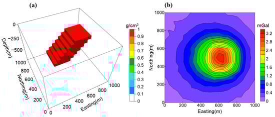
Figure 1.
(a) The dipping dyke model. (b) Gravity data produced by the model shown in Figure 1a. The data set is contaminated by uncorrelated Gaussian noise whose standard deviation is equal to 2% of the accurate datum magnitude plus 0.01 mGal.
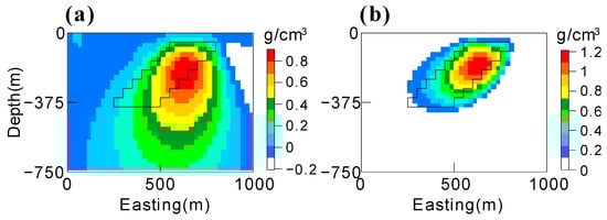
Figure 2.
Central cross-sections at northing = 500 m through the models achieved by inverting the gravity data in Figure 1b using (a) the unconstrained and (b) the positivity-constrained l2-norm inversion. The black lines indicate the position of the true model.
2.3. Model Objective Function
In potential field inversion, l2-norm is a common choice for model objective function [,,,]. Minimizing an l2-norm of the model and/or its spatial derivatives results in a linear system of equations to be solved. Such a minimization is fast and stable, and the resulting solution is smooth. Non-l2-norms are also widely used and generally yield a piecewise-constant or blocky solution. Farquharson [,] minimizes the l1-norms of the model and its spatial derivatives. Last and Kubik [] and Portniaguine and Zhdanov [] minimize a minimum support functional of the model. Portniaguine and Zhdanov [] minimize a minimum gradient support functional of the model. Pilkington [] minimizes the Cauchy norm of the model. Boulanger and Chouteau [] and Fournier and Oldenburg [] minimize mixed-norms of the model. Different choices of model objective function will produce different results.
In Figure 2a, we can observe that the unconstrained l2-norm inversion of a positive anomaly yields many unwanted small negative values in the solution. Based on this observation, we suggest using lp-norm (0 < p < 2) inversion to minimize the effect of negative values because small values in the solution will lead to large penalties with the decrease in p. The difficult lp-norm (0 < p < 2) inversion lies in the choice of p. A large p value will improve the results very little, while a small p value will destroy the smoothness of a solution and yield unrealistically large values in the solution. Therefore, we should choose a proper p value, which not only minimizes the effect of negative values, but also maintains the smoothness of the solution.
2.4. Inverse Problem
The total objective function of gravity lp-norm inversion is defined as
where is a data misfit, is a model norm, and μ is a regularization parameter. The data misfit is defined as
where D is a diagonal data-weighting matrix. Its diagonal element dii is the reciprocal of the estimated noise standard deviation of the ith datum. The model norm is defined as
where W is a diagonal depth-weighting matrix []. Its diagonal element wii is given by Equation (2).
Equation (3) is solved by using the iteratively reweighed least squares (IRLS) technique. The IRLS technique transforms the nonlinear lp-norm inversion into a sequence of linear l2-norm inverse problem [,,,,]. The objective function at the kth iteration is given by
where R(k) is a diagonal reweighting matrix formed by the solution of the previous iteration, and its ith diagonal element is given by
When mi(k−1) = 0, Equation (7) is undefined. To avoid such singularities, Equation (7) is modified by
where ε is a small positive value and generally set to 10−10 in our code. M(0) is set to 1, which means the iteration is started with an unweighted l2-norm solution. Minimizing Equation (6) yields the final iterative equation
Equation (9) can be solved by the conjugate gradient method.
3. Choosing Proper β and p Values
To choose proper β and p values for the artifact-free inversion of gravity data, we need to understand the effect of the depth-weighting function and lp-norm minimization on the inversion results. We used different combinations of β and p values (β values range from 0.2 to 2, with an interval of 0.2; p values range from 1 to 2, with an interval of 0.1) to perform 110 inversions of the gravity anomaly (Figure 1b) generated by the aforementioned dipping slab model (Figure 1a). Due to space limitations, we only show 12 inversion results, with combinations of β = (0.2, 0.8, 1.4, 2) and p = (1, 1.5, 2), in Figure 3.
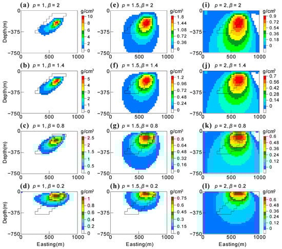
Figure 3.
Cross-sections at northing = 500 m through the models, achieved by inverting the gravity data in Figure 1b using different combinations of β and p values. (a–d) p values equal to 1 and β values vary. (e–h) p values equal to 1.5 and β values vary. (i–l) p values equal to 2 and β values vary. The black lines indicate the position of the true model.
To understand the effect of β on the inversion results, we observed the inversion results with a fixed p value and varying β values. In the third column, from bottom to top, the p values equal to 2 and the β values increase from 0.2 to 2. As the values of β increase, the recovered models are characterized by larger depth extents, larger maximum values, and larger volumes. We can observe a similar pattern for the models in the other two columns. Moreover, with the decrease in p values, the impact of β values on the depth extents and volumes decreases, whereas the maximum values increase. For example, when p = 1, the recovered models with different β values have similar depth extents and volumes but very different maximum values.
To understand the effect of p on the inversion results, we observe the inversion result with a fixed β value and varying p values. In the first row, from right to left, the β values equal to 2 and the p values decrease from 2 to 1. As the p values decrease, the recovered models are characterized by their smaller depth extents, smaller volumes, more evident dipping structures, and larger maximum values. We can observe a similar pattern for the models in the other two rows. Moreover, with the decrease in β values, the impact of p values on the depth extents, volumes, and maximum values is decreasing.
To understand the effect of the p and β values more quantitatively, we calculated the model errors between all the recovered models and the true one using a relative l1-norm
and a relative l2-norm
where mr and mt represent the recovered model and the true one, respectively. Figure 4a,b show the recovered errors of the dipping dyke model with all 110 combinations of β and p values using Equations (11) and (12), respectively.
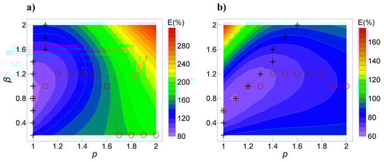
Figure 4.
Recovered errors (in percent) of the dipping dyke model with all 110 combinations of β and p values using (a) a relative l1-norm and (b) a relative l2-norm. The plus symbols represent the position corresponding to the minimum error for a fixed β value and different p values. The cycle symbols represent the position corresponding to the minimum error for a fixed p value and different β values.
We first used the relative l1-norm to evaluate the model errors based on Figure 4a. We can observe that the minimum errors for fixed β values are obtained when p = 1 or 1.1, whereas the minimum errors for fixed p values are characterized by a step curve. For p values ranging from 1.7 to 2, the minimum errors are obtained when β = 0.2. For p values ranging from 1 to 1.6, the minimum errors are obtained when β = (0.8, 1.0, 1.2). The minimum error for all p and β values is obtained when p = 1 and β = 0.8.
We can then use the relative l2-norm to evaluate the model errors based on Figure 4b. First, we investigate the minimum errors for fixed β values. For β = 2, the minimum error is obtained when p = 1.6. With the decrease in β values, the p values corresponding to the minimum errors are also reduced. For , the minimum errors are obtained when p = 1. For fixed p values, the minimum errors are obtained when . The minimum error for all p and β values is obtained when p = 1.1 and β = 0.8.
Based on the above analysis, we suggest that and will produce a reasonable model. The recovered models with minimum errors are also shown in Figure 5. Both models are similar to the positivity-constrained inversion result (Figure 2b) and bear a strong resemblance to the real one. The model based on the minimum relative l1-norm error (Figure 5a) is compact and has a higher maximum value (2.6 g/cm3) compared with the true one (1 g/cm3). The model based on the minimum relative l2-norm (Figure 5b) is a little fuzzy and has a maximum value that is closer to the true one.
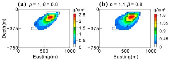
Figure 5.
Recovered dipping dyke models with minimum errors based on (a) a relative l1-norm and (b) a relative l2-norm.
4. Synthetic Example
To verify the validity of the suggested β and p values, we inverted the gravity data produced by the model consisting of two dipping dykes (Figure 6a). The data set (Figure 6b) covers a 41 × 21 grid of 50 m and 100 m spacing along easting and northing, respectively. It is contaminated by uncorrelated Gaussian noise whose standard deviation is equal to 2% of the accurate datum magnitude plus 0.05 mGal. The densities of the east and west dykes are 0.8 and 1 g/cm3, respectively. The corresponding model region is divided into 40 × 40 × 30 cubes of 50 m on each side.
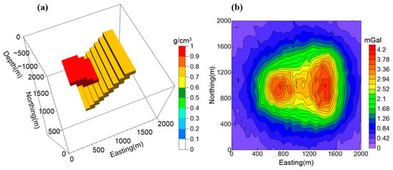
Figure 6.
(a) The model composed of two dipping dykes. (b) Gravity data produced by the model shown in Figure 6a. The data set is contaminated by uncorrelated Gaussian noise whose standard deviation is equal to 2% of the accurate datum magnitude plus 0.05 mGal.
We first invert the gravity data in Figure 6b using unconstrained and positivity-constrained l2-norm inversions, respectively. Both inversion results (Figure 7) show the existence of the two sources. However, the positivity-constrained l2-norm inversion produce more accurate distributions of the two sources.
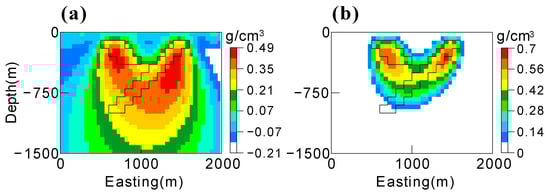
Figure 7.
Central cross-sections at northing = 1000 m through the models achieved by inverting the gravity data in Figure 6b using (a) the unconstrained and (b) the positivity-constrained l2-norm inversion. The black lines indicate the position of the true model.
We then used different combinations of β and p values (β values range from 0.2 to 2, with an interval of 0.2; p values range from 1 to 2, with an interval of 0.1) to perform 110 lp-norm inversions of the data in Figure 6b. The corresponding model errors calculated based on Equations (10) and (11) are shown in Figure 8a,b, respectively. Compared with Figure 4, Figure 8 shows a similar but not identical pattern. For this example, the minimum relative l1-norm error is obtained when p = 1 and β = 1 and the minimum relative l2-norm error is obtained when p = 1.1 and β = 0.6, which are slightly different to the errors in Figure 4. However, the p values still lie in [1, 1.1] and β values still lie in [0.6, 1.2]. The recovered models with minimum errors are also shown in Figure 9. Both models are similar to the positivity-constrained inversion results (Figure 7b) and bear a strong resemblance to the real one.
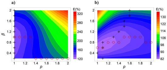
Figure 8.
Recovered errors (in percent) of the model consisting of two dipping dykes with all 110 combinations of β and p values using (a) a relative l1-norm and (b) a relative l2-norm. The symbol descriptions are the same as those in Figure 4.
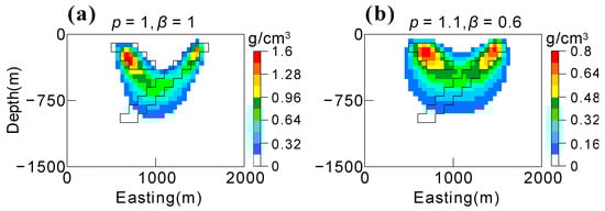
Figure 9.
Recovered models consisting of two dipping dykes with minimum errors based on (a) a relative l1-norm and (b) a relative l2-norm.
5. Field Example
We then applied the proposed strategy to the inversion of gravity data measured over a Layikeleke iron–copper skarn deposit, Xinjiang, China [,]. The ore body is located in the fracture of the lower Devonian volcanic rocks. The host rocks for the ore body include actinolite, diopside, and garnet, which contain abundant magnetite and chalcopyrite. Rock density logging data show that the average density of the ore body (4.0 g/cm3) is evidently higher than the density of surrounding rocks (2.8 g/cm3).
Figure 10a shows the Bouguer gravity anomaly of the deposit, which is gridded into a 101 × 61 grid of 10 m spacing and covers a region of 0.6 km2. In Figure 10a, we can see that the Bouguer anomaly mainly reflects the long wavelength information and contains little information regarding the shallow surface. To extract the local gravity anomaly produced by the ore body located in the shallow surface, we separated the Bouguer anomaly using an inversion-based method. The subsurface was first divided into 20 × 20 × 20 cells to a depth of 640 m. Using lp-norm inversion with p = 1.05 and β = 0.9, we obtained the density distribution within these cells. The regional anomaly was determined by forward modelling of the cells located at depths below 100 m. The residual anomaly (Figure 10b) used to perform the following inversions was calculated by subtracting the regional anomaly from the Bouguer anomaly.
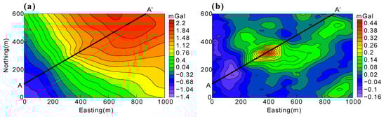
Figure 10.
(a) The Bouguer gravity data of the study region. (b) The residual gravity data calculated by an inversion-based method. The black lines show the positions of the cross-section (AA′) of Figure 11.
We carried out two inversions for the gravity anomalies in Figure 10b using an unconstrained l2-norm inversion and lp-norm inversion with p = 1.05 and β = 0.9, respectively. The model region was discretized into 100 × 60 × 32 cubes of 10 m on each side. The noise of each datum was assumed to be equal to 2% of its magnitude plus 0.004 mGal.
Figure 11a,b display slices produced by the unconstrained l2-norm inversion. The maximum value of the recovered density distribution is about 0.2 g/cm3, which is much lower than the value of the true density contrast (1.2 g/cm3). The recovered model also possesses a broader range of vertical extension compared with the known ore body. Figure 11c,d presents the results of the unconstrained lp-norm inversion with p = 1.05 and β = 0.9. The maximum value of recovered density distribution is about 0.8 g/cm3, which is closer to the value of the true density contrast (1.2 g/cm3). The vertical extension of the model is also in good agreement with that of the known ore body. In addition, both models failed to recover the tail of the ore body. Numerical tests show that this is mainly because the gravity response of the tail is canceled by the response of the adjacent negative source.
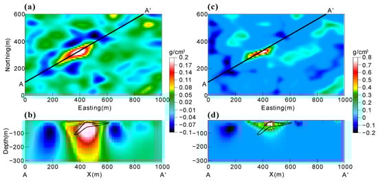
Figure 11.
Plan sections at depth = 45 m and cross-sections of AA′ through the models, achieved by inverting the gravity data in Figure 10b using (a,b) unconstrained l2-norm inversion and (c,d) lp-norm inversion with p = 1.05 and β = 0.9. The black lines in (b,d) indicate the positions of the ore body.
6. Conclusions
An unconstrained l2-norm inversion of gravity data will produce a smooth model. However, this model may contain redundant structures and artifacts. If the gravity anomaly is produced by purely positive sources, one can employ a positivity-constrained l2-norm inversion to eliminate spurious structures and thus improve the solution. In this paper, we developed a strategy that combines unconstrained lp-norm inversion and a careful adjustment of the depth-weighting function to refine the results. Synthetic examples indicate that the results of unconstrained lp-norm inversion are similar to those of a positivity-constrained l2-norm inversion. Therefore, when the gravity data are caused by both positive and negative sources, the unconstrained lp-norm inversion has the potential to recover more reliable information compared with an unconstrained l2-norm inversion method.
Author Contributions
Conceptualization, Z.L.; methodology, Z.L.; validation, Z.L.; formal analysis, Z.L.; investigation, Z.L.; writing—original draft preparation, Z.L. and C.Y.; writing—review and editing, Z.L. and C.Y.; visualization, Z.L.; supervision, C.Y.; project administration, C.Y.; funding acquisition, Z.L and C.Y. All authors have read and agreed to the published version of the manuscript.
Funding
This research was supported by National Natural Science Foundation of China (42004121), Hebei Natural Science Foundation (D2020402009), and National Key Research and Development Program of China (2021YFB3900200).
Data Availability Statement
Not applicable.
Acknowledgments
We would like to thank Jiayong Yan from Chinese Academy of Geological Sciences for providing the real data used in this research.
Conflicts of Interest
The authors declare no conflict of interest.
References
- Blakely, R.J. Potential Theory in Gravity and Magnetic Applications, 1st ed.; Cambridge University Press: Cambridge, UK, 1995; pp. 59–61. [Google Scholar]
- Li, Y.; Oldenburg, D.W. 3-D inversion of gravity data. Geophysics 1998, 63, 109–119. [Google Scholar] [CrossRef]
- Last, B.J.; Kubik, K. Compact gravity inversion. Geophysics 1983, 48, 713–721. [Google Scholar] [CrossRef]
- Portniaguine, O.; Zhdanov, M.S. Focusing geophysical inversion images. Geophysics 1999, 64, 874–887. [Google Scholar] [CrossRef]
- Camacho, A.G.; Montesinos, F.G.; Vieira, R. Gravity inversion by means of growing bodies. Geophysics 2000, 65, 95–101. [Google Scholar] [CrossRef]
- Portniaguine, O.; Zhdanov, M.S. 3-D magnetic inversion with data compression and image focusing. Geophysics 2002, 67, 1532–1541. [Google Scholar] [CrossRef]
- Krahenbuhl, R.A.; Li, Y. Inversion of gravity data using a binary formulation. Geophys. J. Int. 2006, 167, 543–556. [Google Scholar] [CrossRef]
- Uieda, L.; Barbosa, V.C.F. Robust 3D gravity gradient inversion by planting anomalous densities. Geophysics 2012, 77, G55–G66. [Google Scholar] [CrossRef]
- Lu, W.; Qian, J. A local level-set method for 3D inversion of gravity-gradient data. Geophysics 2015, 80, G35–G51. [Google Scholar] [CrossRef]
- Guillen, A.; Menichetti, V. Gravity and magnetic inversion with minimization of a specific functional. Geophysics 1984, 49, 1354–1360. [Google Scholar] [CrossRef]
- Barbosa, V.C.F.; Silva, J.B.C. Generalized compact gravity inversion. Geophysics 1994, 59, 57–68. [Google Scholar] [CrossRef]
- Li, Y.; Oldenburg, D.W. Incorporating geological dip information into geophysical inversions. Geophysics 2000, 65, 148–157. [Google Scholar] [CrossRef]
- Lelievre, P.G.; Oldenburg, D.W. A comprehensive study of including structural orientation information in geophysical inversions. Geophys. J. Int. 2009, 178, 623–637. [Google Scholar] [CrossRef]
- Zhou, J.; Revil, A.; Karaoulis, M.; Hale, D.; Doetsch, J.; Cuttler, S. Image-guided inversion of electrical resistivity data. Geophys. J. Int. 2014, 197, 292–309. [Google Scholar] [CrossRef]
- Lines, L.R.; Schultz, A.K.; Treitel, S. Cooperative inversion of geophysical data. Geophysics 1988, 53, 8–20. [Google Scholar] [CrossRef]
- Gallardo, L.A.; Meju, M.A. Joint two-dimensional DC resistivity and seismic travel time inversion with cross-gradients constraints. J. Geophys. Res. 2004, 109, B03311. [Google Scholar] [CrossRef]
- Lelièvre, P.G.; Farquharson, C.G.; Hurich, C.A. Joint inversion of seismic traveltimes and gravity data on unstructured grids with application to mineral exploration. Geophysics 2012, 77, K1–K15. [Google Scholar] [CrossRef]
- Li, Y.; Oldenburg, D.W. 3-D inversion of magnetic data. Geophysics 1996, 61, 394–408. [Google Scholar] [CrossRef]
- Pilkington, M. 3D magnetic data-space inversion with sparseness constraints. Geophysics 2009, 74, L7–L15. [Google Scholar] [CrossRef]
- Farquharson, C.G.; Oldenburg, D.W. Non-linear inversion using general measures of data misfit and model structure. Geophys. J. Int. 1998, 134, 213–227. [Google Scholar] [CrossRef]
- Kirkendall, B.; Li, Y.; Oldenburg, D. Imaging cargo containers using gravity gradiometry. IEEE Trans. Geosci. Remote Sens. 2007, 45, 1786–1797. [Google Scholar] [CrossRef]
- Farquharson, C.G. Constructing piecewise-constant models in multidimensional minimum-structure inversions. Geophysics 2008, 73, K1–K9. [Google Scholar] [CrossRef]
- Sun, J.; Li, Y. Multidomain petrophysically constrained inversion and geology differentiation using guided fuzzy c-means clustering. Geophysics 2015, 80, ID1–ID18. [Google Scholar] [CrossRef]
- Fournier, D.; Oldenburg, D.W. Inversion using spatially variable mixed ℓp norms. Geophys. J. Int. 2019, 218, 268–282. [Google Scholar] [CrossRef]
- Utsugi, M. 3-D inversion of magnetic data based on the L1–L2 norm regularization. Earth Planets Space 2019, 71, 73. [Google Scholar] [CrossRef]
- Sun, J.; Wei, X. Research Note: Recovering sparse models in 3D potential-field inversion without bound dependence or staircasing problems using a mixed Lp norm regularization. Geophys. Prospect. 2021, 69, 901–910. [Google Scholar] [CrossRef]
- Nagy, D. The gravitational attraction of a right rectangular prism. Geophysics 1966, 31, 362–371. [Google Scholar] [CrossRef]
- Li, X.; Chouteau, M. Three-dimensional gravity modeling in all space. Surv. Geophys. 1998, 19, 339–368. [Google Scholar] [CrossRef]
- Boulanger, O.; Chouteau, M. Constraints in 3D gravity inversion. Geophys. Prospect. 2001, 49, 265–280. [Google Scholar] [CrossRef]
- Cella, F.; Fedi, M. Inversion of potential field data using the structural index as weighting function rate decay. Geophys. Prospect. 2012, 60, 313–336. [Google Scholar] [CrossRef]
- Li, Y.; Oldenburg, D.W. Joint inversion of surface and three-component borehole magnetic data. Geophysics 2000, 65, 540–552. [Google Scholar] [CrossRef]
- Oldenburg, D.W.; Li, Y. Inversion for applied geophysics: A tutorial. In Near-Surface Geophysics; Society of Exploration Geophysicists: Houston, TX, USA, 2005; pp. 89–150. [Google Scholar]
- Barbosa, V.C.F.; Silva, J.B.C.; Medeiros, W.E. Practical applications of uniqueness theorems in gravimetry: Part II—Pragmatic incorporation of concrete geologic information. Geophysics 2002, 67, 795–800. [Google Scholar] [CrossRef]
- Pilkington, M. 3-D magnetic imaging using conjugate gradients. Geophysics 1997, 62, 1132–1142. [Google Scholar] [CrossRef]
- Lelievre, P.G.; Oldenburg, D.W. Magnetic forward modelling and inversion for high susceptibility. Geophys. J. Int. 2006, 166, 76–90. [Google Scholar] [CrossRef]
- Beaton, A.E.; Tukey, J.W. The fitting of power series, meaning polynomials, illustrated on band-spectroscopic data. Technometrics 1974, 16, 147–185. [Google Scholar] [CrossRef]
- Holland, P.W.; Welsch, R.E. Robust regression using iteratively reweighted least-squares. Commun. Stat. Theory Methods 1977, 6, 813–827. [Google Scholar] [CrossRef]
- Rao, B.D.; Kreutz-Delgado, K. An affine scaling methodology for best basis selection. IEEE Trans. Signal Process. 1999, 47, 187–200. [Google Scholar] [CrossRef]
- Yan, J.Y.; Meng, G.X.; Yang, Y.Q.; Deng, Z.; Zhao, J.H.; Tang, H.J. Discovery and metallogenic characteristics of Layikeleke magmatic skarn type of rich copper-iron deposit, Eastern Junggar, Xinjiang. Geol. Rev. 2017, 63, 413–426. [Google Scholar]
- Cui, Y.; Guo, L. A wavenumber-domain iterative approach for rapid 3-D imaging of gravity anomalies and gradients. IEEE Access 2019, 7, 34179–34188. [Google Scholar] [CrossRef]
Disclaimer/Publisher’s Note: The statements, opinions and data contained in all publications are solely those of the individual author(s) and contributor(s) and not of MDPI and/or the editor(s). MDPI and/or the editor(s) disclaim responsibility for any injury to people or property resulting from any ideas, methods, instructions or products referred to in the content. |
© 2023 by the authors. Licensee MDPI, Basel, Switzerland. This article is an open access article distributed under the terms and conditions of the Creative Commons Attribution (CC BY) license (https://creativecommons.org/licenses/by/4.0/).