First Ocean Wave Retrieval from HISEA-1 SAR Imagery through an Improved Semi-Automatic Empirical Model

Abstract

The HISEA-1 synthetic aperture radar (SAR) minisatellite has been orbiting for over two years since its launch in 2020, acquiring numerous high-resolution images independent of weather and daylight. A typical and important application is the observation of ocean waves, essential ocean dynamical phenomena. Here, we proposed a new semi-automatic empirical method to retrieve ocean wave parameters from HISEA-1 images. We first applied some automated processing methods to remove non-wave information and artifacts, which largely improves the efficiency and robustness. Then, we developed an empirical model to retrieve significant wave height (SWH) by considering the dependence of SWH on azimuth cut-off, wind speed, and information extracted from the cross-spectrum. Comparisons with the Wavewatch III (WW3) data show that the performance of the proposed model significantly improved compared to the previous semi-empirical model; the root mean square error, correlation, and scattering index are 0.45 m (0.63 m), 0.87 (0.75), and 18% (26%), respectively. Our results are also consistent well with those from the altimeter measurements. Further case studies show that this new ocean wave model is reliable even under typhoon conditions. This work first provides accurate ocean-wave products from HISEA-1 SAR data and demonstrates its ability to perform high-resolution observation of coasts and oceans.

1. Introduction

Ocean wave is an ubiquitous and important phenomenon in global oceans which plays an important role in marine transport, ocean dynamics, coastal engineering, and even wave climate change [1]. Global ocean waves have a large range of spatial and temporal scales, from capillary wave (centimeter) to planetary wave (hundred kilometers), and they are randomly distributed and interacting with each other [2]. To better describe their general characteristics, some main ocean wave parameters are put forward, including the significant wave height (SWH or Hs), average wave period, and wave direction. The observation of the global ocean wave and the retrieval of its main parameters are essential for understanding their distributions, the interaction with other ocean variables, and their role in ocean dynamics and climate change [2,3].

SWH is defined as an average measurement of the highest third of the waves, which represents the shape and energy of the wave and thus is one of the most important parameters of ocean waves. Ocean wave can be measured through an in situ method such as buoys, however data from in situ measurements are too sparse and short-living to provide enough temporal and spatial information. Ocean wave can also be observed remotely, such as from spaceborne satellites, which have the advantages of large spatial and longer temporal coverage, among which, synthetic aperture radar (SAR) is an active microwave radar that can provide all-weather, all-time, and high-resolution observation of the radar cross section (RCS, or reflectivity) of the earth’s surface. SAR can take global images of the waves, retrieve the wave spectrum and obtain all the information about the waves. The mechanism of SAR imaging the sea surface has been widely recognized since the launch of SEASAT, including tilt modulation, hydrodynamic modulation, and velocity bunching [4,5,6].

According to previous studies, the method of retrieving SWH from SAR can be divided into two categories. For the conventional method, wave spectrum is first inversed from SAR images and then ocean wave parameters can be easily obtained from the wave spectrum through some simple integration. The problem of this approach is that the inversion of the wave spectrum is difficult due to the nonlinear effects of velocity bunching [7,8,9] and during which a priori information is usually required to resolve the 180° ambiguity of wave propagation direction. The replacement of the image spectrum inversion with the cross spectra based on transfer functions was a breakthrough in this field, after which several methods were proposed to retrieve directional wave spectra from SAR images without model direction information [10,11,12]. Another approach is to build up an algorithm to extract the wave parameters directly from the SAR images, without dealing with the complex wave spectrum inversion. An empirical algorithm was first proposed to retrieve SWH and wave period from the ERS-2 wave mode, called CWAVE_ERS, which is based on the multiple-regression method of 22 input parameters from SAR and the image spectrum [13]. This model showed great agreement with the model and buoy without external information, and was extended to other C-band satellite wave modes such as ENVISAT [14], and Sentinel-1 [15], as well as for Wave Mode (WM) that is designed for traditional C-band satellites.

Velocity bunching is nonlinear, resulting in an azimuthal cut-off and distorting the wave energy in the spectrum. However, the SAR has a limitation in the azimuthal direction when imaging the sea surface, resulting in the distortion of wave energy or loss in spectra beyond a specific wavelength. This is termed as the azimuth wavelength cut-off or azimuth cut-off. This effect is positively correlated to the satellite slant-range to velocity ratio [16]. Although the azimuth cut-off is not the basic characteristic of SAR, it provides a useful quantity of sea state information [17]. Regarding the azimuth cut-off, empirical algorithms with simplified parameters have also been proposed for different SAR modes and missions [18,19,20,21,22,23,24]. Unlike the tuning algorithm with large datasets, Wang et al. [25] proposed a semi-empirical expression that associates the SWH with the azimuth cut-off, peak wavelength, and wave propagation direction, and their method is suitable for any SAR data. Usually, SAR image tuning in empirical algorithms is conducted in open oceans, where homogeneity detection is employed to exclude SAR images with non-wave influences [13]. Even open-ocean WM data comprise microconvective cells, rain cells, low-wind areas, and other non-wave signals, which pose a major obstacle in the retrieval of wave information from SAR images [26]. Some studies have focused on coastal wave retrieval [27,28], where the selection of nearshore subscenes with pure sea state is difficult compared to that in open water owing to several common artifacts such as ships and wind farms [29].

On 22 December 2020, the HISEA-1 C-band minisatellite was launched. It provides up to 1-m resolution with 100 km swath. Detailed information can be found in [30]. Up to now, thousands of SAR images have been accumulated near the shore. High-resolution SAR images from HISEA-1 have been used for many coastal and ocean applications, such as ship detection [31] and flood mapping segmentation [32] through deep learning. Unlike conventional C-band SAR satellites with a mass of thousands of kilograms, miniaturized satellites can form constellations at low cost and improve the temporal resolution of the ocean. After HISEA-1, some SAR minisatellites have been launched, such as Chaohu-1 in February 2022.

In this paper, we provide a new wave-retrieval model for HISEA-1 SAR striping mode (SM) images and first obtain ocean wave parameters over the nearshore seas of Fujian from this satellite. We first filter the artifacts present in nearshore HISEA-1 images and then propose an empirical algorithm to retrieve the SWH mainly based on the relationship between the SWH and azimuth cut-off and the spectrum parameters. We evaluated the algorithm’s performance for two cases: in nearshore and high sea-state conditions. The remainder of this paper is organized as follows. Section 2 introduces the HISEA-1 SAR and validation data. The theoretical methodology for developing the empirical algorithm and data processing is presented in Section 3. In Section 4, the results are validated using model and altimeter measurements. Section 5 presents the discussion of the application and performance of the empirical model in coastal and high sea states, and Section 6 presents the conclusions.

2. Data

2.1. HISEA-1 SAR Images

HISEA-1 is a C-band (5.4 GHz) SAR minisatellite with VV single polarization for ocean and coastal observations. It possesses a sun-synchronous orbit with an orbital altitude of approximately 500 km, which is relatively low compared with those of other C-band SAR satellites. Detailed information for satellite platform parameters and imaging mode parameters of HISEA-1 can be found in [33]. This minisatellite comprises four imaging modes [30], as listed in

Table 1. Imaging mode of HISEA-1.

Mode	Striping	Spotlight	Narrow ScanSAR	Extra ScanSAR
Swath/km	20	5 × 5	50	100
Resolution/m	3	1	10	20
Polarization	VV	VV	VV	VV

, among which the striping mode has a resolution of 3 m and 20 km swath. The SAR data period used in this study ranges from December 2022 to February 2023.

The radiometric calibration of HISEA-1 was achieved using a calibration look-up table and can be formulated as follows:

$${\sigma }^0=\frac{{\left|D{N}_i\right|}^2}{A_i^2}$$

(1)

where ${\sigma }^0$ is NRCS, $A_i$ is the calibration constant, and $DN$ is grayscale. For pixel $i$ between the points in the look-up table, $A_i$ is obtained through bilinear interpolation.

2.2. Reference Data

2.2.1. Buoy Data

The buoy data are more reliable as the in-situ measurement obtained from the Fujian Provincial Marine Forecast Station. As shown in Figure 1a, the buoys are located in SAR data coverage, mainly in the Taiwan Strait. The buoy provides the SWH and 10-m wind speed (U10) every 30 min. These data can be used as the validation data for the WW3 model comprising SWH and ERA5 wind speed, and compared with SAR results in the case study.

2.2.2. WAVEWATCH III Data

The WAVEWATCH III (WW3) model data used in this study is a third-generation wave model developed by the National Oceanic and Atmospheric Administration (NOAA). The model provides hourly global wave parameters with a 0.167° × 0.167° grid.

2.2.3. MFWAM Data

To compare the SWH retrieved from subscenes with high-resolution model outputs, we selected data from the Météo-France wave model (MFWAM), which is a third-generation wave model, using a new dissipation term developed by Ardhuin et al. [34]. The MFWAM has a spatial resolution of 1/12° × 1/12° and a 3 h temporal resolution. The model output parameters used in the current study are the total SWH and wave direction, which were compared with the data of HISEA-1 under the high sea state.

2.2.4. ERA5 Reanalysis

ERA5 is the fifth generation of global climate reanalysis data published by the European Centre for Medium-Range Weather Forecasts, covering the period from 1950 to the present. This dataset provides hourly values of land, atmospheric, and oceanic variables, replacing the original ERA-Interim reanalysis data. For pre-interpolated atmospheric data (e.g., wind speed), the dataset has a resolution of up to 0.25° × 0.25°, while providing a resolution of 0.5° × 0.5° for ocean waves. We used ERA5 wind speed as an auxiliary input to the empirical algorithm.

2.2.5. Altimeter Measurement

Altimeters can measure the global SWH, and their measurements have been verified by buoy and model data. In this paper, we collocated HISEA-1 images with multiple altimeter missions with a time window of 1 h and a spatial window of overlapping or 1° parallel orbit. During the HISEA-1 period, four altimeter missions were used for independent validation, namely Jason-3, Sentinel-6A, Sentinel-3A, and Cryosat-2 (detailed SAR-altimeters collocations in Appendix A).

2.3. Model Data Validation with Buoys

For a limited number of buoy–SAR collocations, the model data are taken as the ground truth after being validated through buoy measurements. The following presents the validation results of the interpolated wind-speed data from ERA5 and SWH data from WW3 against buoy measurements in December 2022. Four statistical parameters, namely root mean square error (RMSE), bias, correlation (R), and scattering index (SI), are used to quantify the results:

$$\mathrm{b}\mathrm{ias}=\frac{1}{N}\sum _{i=1}^N\left(y_i-x_i\right)$$

(2)

$$\mathrm{RMSE}=\sqrt{\frac{1}{N}\sum _{i=1}^N{\left(y_i-x_i\right)}^2}$$

(3)

$$\mathrm{R}=\frac{{\sum }_{i=1}^N\left(x_i-⟨x_i⟩\right)\left(y_i-⟨y_i⟩\right)}{\sqrt{{\sum }_{i=1}^N{\left(x_i-⟨x_i⟩\right)}^2{\sum }_{i=1}^N{\left(y_i-⟨y_i⟩\right)}^2}}$$

(4)

$$\mathrm{SI}=\frac{\mathrm{RMSE}}{\overline{x_i}}$$

(5)

where $x_i$ and $y_i$ represent SWHs from reference data and HISEA-1 acquisition, respectively; N is the total number of data points, and 〈 〉 indicates the average operator.

The hourly U10 comparison between the buoy and ERA5 measurements above 2 m/s is shown in Figure 2a, with RMSE, R, and SI of 1.44 m/s, 0.95, and 13%, respectively, revealing that the ERA5 data are underestimated at buoy wind speeds greater than 15 m/s. The validation through the comparison of WW3-based hourly SWH with buoy showed a deviation of −0.23 m, an RMSE of 0.39 m, correlation of 0.95, and SI of 0.14%, with WW3 showing underestimated wave heights for buoy wave heights greater than 4.5 m. The main SWH was concentrated at 2–3 m, as shown in Figure 2b, representing the normal range of SWH in this area during winter. The errors in both comparison results are acceptable, and the WW3 data can be considered as the ground truth to tune the empirical algorithm.

3. Methodology

3.1. Filtering, Detrending, and Bright Target Removals

For the SAR-wave imaging mechanism, under low sea state, small wave height, and wind speed, SAR can scarcely image the wave stripes. Figure 3a shows images under the low sea state with 2 m/s U10 and invisible wave streaks. Figure 3b presents images under the moderate sea state with 8 m/s U10, and the wind streaks are also visible. Figure 3c displays images under the high sea state with over 8-m SWH and over 20 m/s of wind speed. Figure 3d shows the wave refraction and diffraction phenomena occurring on an island in eastern Taiwan. The SAR data used in this study were obtained from SM SLC images.

To tune the HISEA-1 data and obtain reliable results, the following criteria were used in filtering SAR image data for the inversion of the sea state:

• no large area of land in the SAR image;
• the absence of significant atmospheric disturbances and rainfall factors;
• SAR data matched with ERA5 wind speeds greater than 2 m/s and wave heights greater than 0.5 m.

Furthermore, the normalized variance ($nv$) of the SAR image was calculated to check for homogeneity:

$$nv=\mathrm{v}\mathrm{a}\mathrm{r}\left(\frac{I-⟨I⟩}{⟨I⟩}\right)$$

(6)

where $⟨I⟩$ is the average intensity of the SAR data. In addition, this parameter will also be an important parameter in the empirical algorithms due to its strong relationship with the wave conditions in the SAR images. A total of 1590 SAR images were selected after quality control, and Figure 1b shows the location map of HISEA-1 images.

In the open ocean, ocean waves in SAR images acquired by WM are always swell-dominated and have negligible spatial changes. In nearshore, wind sea dominates the sea state and rapidly changes; artifacts are often found in HISEA-1 images, where it is necessary to preprocess the images and depress the noise. Therefore, HISEA-1 SM images are split into several 4096 × 4096 pixels subscenes, which covers approximately 6 × 6 km area, to obtain a better view of the spatial variability of waves and ensure that non-wave information does not interfere with all subscenes.

We reduce the interference of artifacts in the spectrum by detrending and bright target removal. Detrending is the use of Gaussian low-pass filtering on the SLC data. This method removes the average trend and background noise from the image to highlight wave stripes in SAR images.

Bright target removal is realized using a sliding window of 50 × 50 pixels to determine if the intensity is more than 2.3 times above average and replacing the high value in sliding window with the whole image average intensity. Figure 4 shows the comparison before and after the removal of the bright targets, where the non-wave energy density in the cross-spectrum is relatively reduced and the wave component can be clearly distinguished. As observed, although interference information is still present in the low wavenumber region, it can be filtered out by masking the energy in the low wavenumber (wavelength > 400 m), which is usually filtered out by wind streaks and oil film. In the North Sea, approximately 20–25% of subscenes of SAR images can be used for the spectral transformation owing to artifacts [28]. With these steps, the final filtered-out subscenes are approximately 10% of the total, thus greatly improving the availability of nearshore images. Then, the normalized variance is calculated in preprocessing subscenes, for checking the homogeneity.

3.2. Semi-Empirical Model and Its Problems

The SAR imaging in the range is the same as real aperture radar, with tilt, and hydrodynamic modulations, which always involve linear transformation. However, the velocity bunching effect occurs in the azimuth when SAR observation of the Doppler frequency shift is sensitive to the relative velocity between the radar and target. This phenomenon is termed as the azimuth wavelength cut-off, which can be expressed as follows:

$${\lambda }_{\mathrm{co}}=\pi \beta \sqrt{{\rho }^{vv}}$$

(7)

The mean square orbital velocity in the range direction, ${\rho }^{vv}$, can be expressed as

$${\rho }^{vv}={\int }_0^{\mathrm{\infty }}{\int }_0^{2\pi }{⌊T_k^v⌋}^{2}S\left(\omega \right)D\left(\omega ,\phi \right)d\phi d\omega$$

(8)

where $D\left(\omega ,\phi \right)$ is the normalized directional distribution function and $S\left(\omega \right)$ is the wave spectrum. The range velocity transfer function [4], $T_k^v$, is denoted as

$$T_k^v=-\omega \left(\mathit{sin}{\phi }_k\mathit{sin}\theta +i\mathit{cos}\theta \right)$$

(9)

where $\theta$ is the incidence angle.

Based on the derivation and simplification by Wang [25], the semi-empirical relationship between Hs and azimuth cut-off can be written as (in finite water dispersion relation)

$$H_s=C\frac{0.3608}{\beta \sqrt{g}\sqrt{\mathit{tanh}\left(2\pi d/{\lambda }_p\right)}}{\lambda }_c\sqrt{{\lambda }_p}$$

(10)

where ${\lambda }_p$ is the peak wavelength and ${\lambda }_c$ is the azimuth cut-off. The dimensionless coefficient, C, can be expressed as

$$C=\frac{1}{\sqrt{1-0.5 {\mathit{sin}}^2\theta \left[1+\frac{\left(2\pi /2B\right)}{\mathit{sinh}\left(2\pi /2B\right)}\mathit{cos}\left(2\psi \right)\right]}}$$

(11)

Constant B = 2.44, $\psi$ is the peak wave direction to azimuth.

By Equations (10) and (11), the extraction of significant wave heights from HISEA-1 data can be accomplished. Due to the requirement for shallow water depth $d$, GEBCO bathymetry data is employed, while the remaining parameters are derived from SAR images.

The results of the semi-empirical algorithm for some SAR data were compared with those of two model data sets, as shown in Figure 5. Both model data sets exhibit an RMSE of approximately 0.62 m and a scattering coefficient of around 25%. The results indicate an underestimation of the SAR data when the model wave height exceeds 3 m, whereas in the range of 0.5–2 m, the SAR results significantly overestimate the significant wave height. The bias is related to azimuth cut-off wavelength, thus Pramudya et al. [35] proposed an improvement by estimating the cut-off wavelength using dual-polarization data. Semi-empirical algorithms have been used for the validation of ENVISAT WM [25] and Sentinel-1 dual-polarized IW data [35].

An empirical algorithm containing only two parameters, i.e., the azimuth cut-off wavelength, and range-to-velocity ratio, can obtain accurate SWH from the fully polarized Radarsat-2 data [18]. According to the azimuth cut-off from the 10-year ENVISAT data, the azimuth cut-off fitted using Gaussian functions has bias with respect to the buoy measurement, which has been shown to be related to wind speed and normalized variance [17]. Therefore, wind speed should be included as a parameter in empirical algorithms dominated by the cut-off wavelength; note that in this study, the wind speed was not taken from HISEA-1 images. The $nv$ in Equation (6) from the SAR image was tested by CWAVE in several SAR WM data.

Moreover, ${\lambda }_c/\beta$, and incidence angle are considered in our algorithm based on findings of previous studies [25,36,37,38]. We used $\mathit{tan}\theta$ to represent the effect of the incidence angle, which is a larger value than $sin \theta$. For the wave direction relative to heading $\phi$ ($\phi$ = 0° for wave propagation along azimuth and $\phi$ = 90° for wave propagation along range), $\mathit{cos}2\phi$ was observed to significantly affect the azimuth cut-off [39]. The azimuth cut-off ${\lambda }_c$, peak wavelength ${\lambda }_p$, and wave direction relative to azimuth $\psi$, are considered as the most important parameters, which are obtained from the semi-empirical algorithm.

3.3. An Improved Empirical Model

By summarizing the results of the semi-empirical algorithm and the analyses by previous studies, wind speed and nv should be added to improve the semi-empirical model. A new empirical algorithm for the SWH based on the C-band HISEA-1 can be written as:

$$H_s=C_1\frac{{\lambda }_c}{\beta }\sqrt{{\lambda }_p}+C_2{U}_{10}+C_{3}nv+C_4\mathit{cos}2\phi +C_5\mathit{tan}\theta +C_6$$

(12)

This new empirical algorithm has taken into account of all relevant variables, including the azimuth cut-off, peak wavelength, wind speed, wave direction, and incidence angle, with $C_1-C_6$ being non-zero coefficients to be determined. To complete this model, some more information is required, including cross-spectra calculation, azimuth cut-off estimation, and spectral information.

3.3.1. Cross-Spectra Calculation

In this study, we used cross-spectra rather than the SAR spectrum to extract spectral information. The cross-spectra method was first proposed by Engen and Johnsen [10] and has been the base of Sentinel-1 OSW level-2 product. This method not only solves the 180° ambiguity of the wave propagation direction but also reduces the speckle noise in SAR images. The detailed process of computing cross-spectra from SAR images can be looked up in [40], which is briefly stated as follows. (1) Detrend the intensity by low-frequency filtering and remove bright targets, highlighting wave signature in SLC subscene data with 4096 × 4096 pixels. (2) The subscene is split into 1024 × 1024 pixel sub-subscenes; each sub-subscene overlaps 50% in both range and azimuth so that a total of 7 × 7 sub-subscenes are extracted. (3) Apply the standard fast Fourier transform (FFT) to each sub-subscene and extract three nonoverlapping sub-looks. (4) Apply inverse Fourier transform and obtain intensity sub-look images. (5) Compute spatial averaging of the cross spectra, finally obtaining one cospectrum (0 $\tau$) and two cross-spectra (1 $\tau$ and 2 $\tau$), where $\tau$ represents the look separation time of approximately 0.3 s for HISEA-1.

$$P_s^{\left(m,n\right)}\left(k,\mathsf{\Delta }t\right)=\frac{⟨\left[I^{\left(m\right)}\left(k\right)\right]\cdot {\left[I^{\left(n\right)}\left(k\right)\right]}^{\mathrm{*}}⟩}{⟨I^{\left(m\right)}\left(x\right)⟩\cdot ⟨I^{\left(n\right)}\left(x\right)⟩}-\delta \left(k\right),m,n\in \left[1,2,3\right]$$

(13)

where $\mathsf{\Delta }t$ is the separation time between m and n looks, $\mathsf{\Delta }t=\left|m-n\right|\tau$; $\tau$ is the SAR integration time; * is the complex conjugate; and $\delta \left(k\right)$ is a Dirac Delta function.

3.3.2. Azimuth Cut-Off Estimation

Based on the estimation azimuth cut-off method by Kerbaol et al. [39], we adapted the cross-correlation function to the inverse FFT of the real part of the cross-spectrum and fit it to the Gaussian function. The Gaussian fit function is expressed as

$$C\left(x\right)\sim e^{-{\pi }^2\frac{x^2}{{\lambda }^2}}$$

(14)

where C is the cross-correlation function (solid black line in Figure 6b) from cross-spectra with 1 lag time interval, x denotes the spatial distance in the azimuth direction. In this case, the azimuth cut-off estimation is 80 m, which the SAR image acquired under a low sea state. As the low orbit of HISEA-1, the ratio of range to platform velocity is approximately 75 s, and the cut-off is up to a minimum of 50 m, which significantly reduces the distortion of azimuthal spectral information.

3.3.3. Spectral Information Extraction

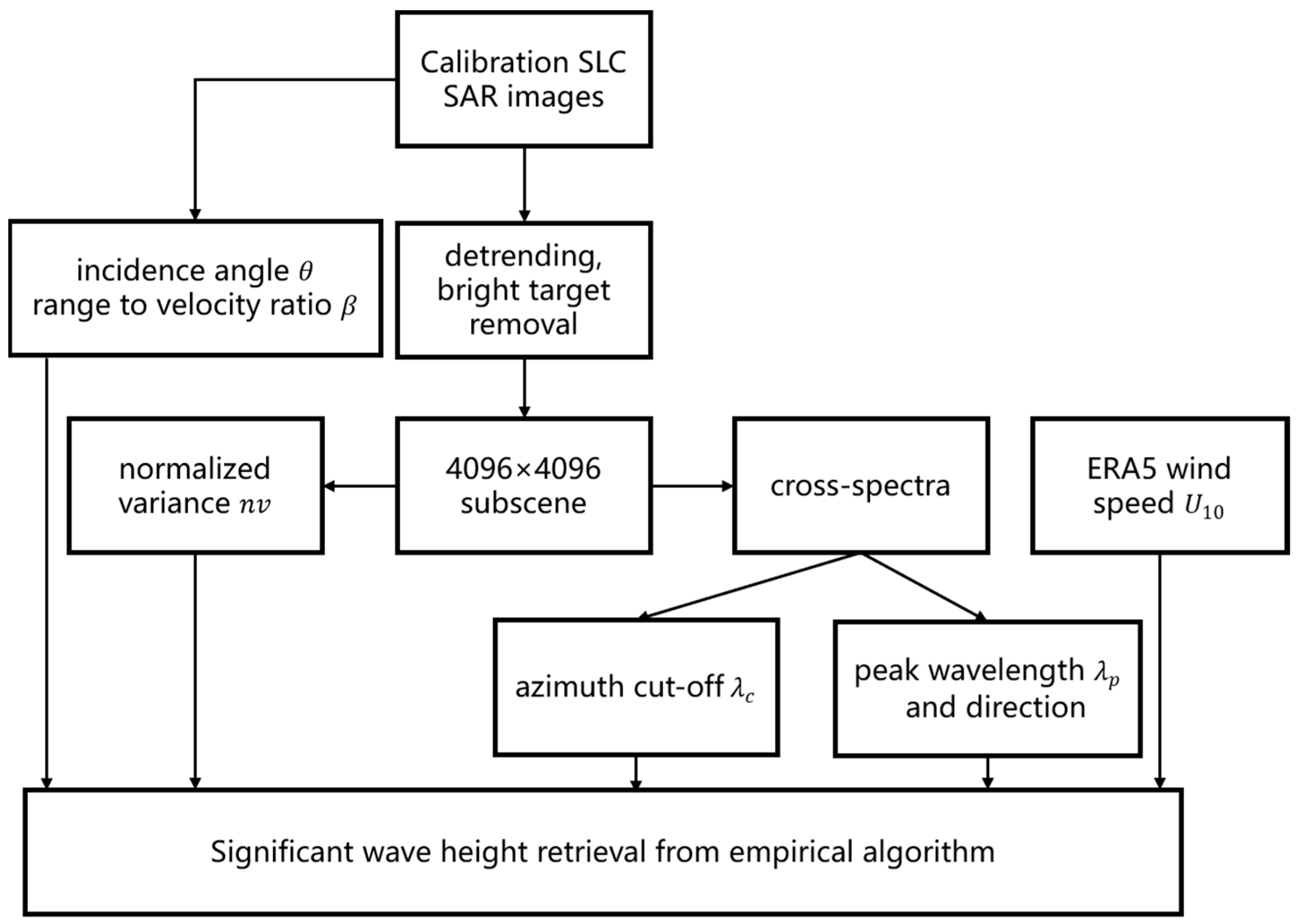
The peak direction in the cross-spectrum was extracted using the Sentinel-1 OSW inversion algorithm [41]. First, the cartesian to logarithmic polar grid transformations converts the cartesian wavenumber into a log–polar grid using bilinear interpolation. Then, spectral partitioning [42] is applied to the cross-spectrum, removing the negative imaginary part. Finally, an integration strategy for extracting the maximum value is employed instead of the simple maximum value extraction to extract peak wave direction and wavelength (see Equations (43)–(46) in [42]).

3.4. Flowchart

Figure 7 presents the general flowchart of the extraction of the SAR and wave parameters, with detailed explanations provided earlier in the text. The main process can be summarized as follows. First, preprocessing includes the calibration and prefiltering of the non-wave information which is a procedure of quality control. Then, the subscene of 4096 × 4096 pixels is used to estimate the cross-spectra that extracted the peak wave information. Finally, the significant wave height can also be extracted from the empirical model.

4. Validation and Performance

The HISEA-1 SAR data were categorized into tuning sets (34%) and validation sets (66%). The six empirical coefficients C1–C6 (see

Table 2. Coefficient of empirical algorithm.

${\mathit{C}}_1$	${\mathit{C}}_2$	${\mathit{C}}_3$	${\mathit{C}}_4$	${\mathit{C}}_5$	${\mathit{C}}_6$
0.04	0.17	0.86	0.11	0.24	−1.74

) were obtained using the least-squares method with WW3 SWH as the reference data. All the histograms of the tuning and validation parameters as well as the comparison results of the tuning dataset are shown in Figure 8, and 89% of collocations of matched U10 from ERA5 are below 15 m/s. A deviation of 0 m, a correlation of 0.88, and a scattering index of 17% were obtained by fitting 5353 SAR subscenes, indicating a good fit of the empirical algorithm to the WW3 model. However, there are only 5 SAR-buoy collocations within three months, we present the results in Appendix B, and we focus on the comparison with the model data and altimeter measurements.

4.1. Comparison with Model Data

The HISEA-1 data from July 2022 to February 2023 were compared with the WW3 data to validate the results of the empirical algorithm. As shown in Figure 9, the results display the RMSE of 0.45 m, correlation of 0.86, and SI of 18%. Compared with the independent MFWAM model, the RMSE, and correlation are 0.54 and 0.83, respectively, which are slightly worse than the values obtained by WW3. Both indicators of validation are close to the accuracy of the CWAVE_S1A inversion of Sentinel-1, indicating that the proposed empirical algorithm can retrieve SWH with good accuracy.

4.2. Comparison with Altimeter Observation

The satellite altimeter spatial sampling is approximately 7 km, which is close to the coverage of the HISEA-1 subscene, which can be formed for comparison. At 02:16 UTC on 23 February 2023, HISEA-1 acquired a set of 38 descending images. Sentinel-3A and Jason-3 passed through the same region at 2:03 and 1:19 UTC, respectively. The time difference between the data of Sentinel-3A altimeter and HISEA-1 was less than 15 min and the tracks were largely parallel (Figure 10a). The meridional variation in the SWH of the altimeter and SAR can be observed spatially across approximately 8° latitude (20°N to 28°N), and the overall lower SWH of the WW3 mode data is displayed in Figure 10. As observed, on the eastern side of Taiwan Island at 24°N 124°E, the wave height between this island and Taiwan Island is relatively small owing to the presence of islands. Further, from 20°N to 24°N, the variation in wave height by HISEA-1 is the same as that measured by the altimeter, both being approximately 1 m higher than the SWH obtained through WW3. Overall, the SAR inversion wave heights are overestimated compared to those by WW3 and are closer to the altimeter results. In addition, the meridional variation of the satellite data is more pronounced compared to that of the WW3 model. In Figure 10a, the orbit of HISEA-1 between Jason-3 and Sentinel-3A is cross and parallel, resulting in approximately 10, and 110 matchups, respectively.

A total of 268 matchups were collated from nine missions of HISEA-1 with four different altimeters. Figure 11 shows the comparison displaying a correlation of 0.86, an RMSE of 0.41 m, and an SI of 17%. The independent altimeter data show good agreement with that of HISEA-1, and the comparison results are close to those of the WW3 model.

5. Application and Case Studies

5.1. Coastal Wave Field Extraction

On 30 December 2022, in a low-medium sea state, HISEA-1 was imaged in the striping mode range from 17.5°N to 25°N in a descending track. A buoy SWH of 3 m was recorded at 2:40, a mere 8 min before SAR imaging, in one of the SAR images in this mission, as shown in Figure 12a. The result of the empirical algorithm from the subscene of A1 is 3 m, which is consistent with the buoy measurement.

To make more effective use of high-resolution images to represent the variability of waves, we extracted sub-subscenes of 2048 × 2048 (A2) and 1024 × 1024 (A3) pixels (shown in Figure 13) from A1. SAR subscenes with different pixels affect the results of the azimuth cut-off wavelength estimation [43]. The spectral information, cut-off wavelength, and SWH of A1, A2, and A3 are listed in

Table 3. Wave information for SAR subscenes with different pixels.

Subscene	Cut-Off (m)	The Peak Direction (°)	Peak Wavelength (m)
A1	164	220.1	158
A2	155	230.0	167.6
A3	119	254.9	142.1

. In this case, the difference in the SWH results from the three different subimages was not significant, differing from the buoy by 0, 0.3, and 0.1 m, respectively.

By splitting into smaller subscenes, a refined spatial variation of the nearshore waves can be depicted. The black frame in Figure 14a shows the SWH from 1024 × 1024 pixels of HISEA-1. Although SWH retrieved from HISEA-1 is slightly lower than that from WW3 in the SAR descending coverage, the buoy located in the SAR image shows a similar SWH with HISEA-1, with only 0.1 m deviation. In contrast, the WW3 data show a difference with respect to several buoys in the Taiwan Strait.

The wave variation evident near the land is shown in Figure 14b. A few sub-subscenes were filtered out by homogeneity detection, with some outliers, demonstrating that image processing can resolve much of the non-wave information nearshore. Some outliers may result from the dark pixels at the edges of the original SAR image. This aspect will need further improvement when processing the images.

Nevertheless, in this case, HISEA-1 can provide much detail and a reliable source of high-resolution data for nearshore wave studies.

5.2. Wave Retrieval under Typhoon

At 12:58 p.m. UTC on 15 September 2022, HISEA-1 acquired 10 SM SAR images, with the typhoon center located to the southeast of the SAR coverage, and the wave propagation direction from the mode data almost following the SAR range direction. Figure 15a shows the SWHs of the MFWAM model at 12:00, ranging from 4.5 to 6.5 m within the SAR coverage. The black arrow indicates the peak wave direction of the model, and the scatters represent the SWH of the SAR images. The wave propagation directions from the SAR crossspectra (white arrow) are almost consistent with the MFWAM peak wave direction. The results of the empirical algorithm for this mission of SAR data show an overall bias in the inversion under a typhoon of approximately −1 m in Figure 15b. Li et al. [44] proved that the ERA5 wind speed exhibits a significant underestimation under high wind conditions, which partly explains the error. By using the wind field from the cross-calibrated multiplatform (CCMP) instead of the ERA5 at 12:00 on 15 September, the empirical algorithm results are shown in Figure 15c. The RMSE is reduced from 1.09 to 0.73 m along with the deviation and scattering coefficients. By replacing the CCMP wind speed with the ERA5 wind speed, the empirical algorithm results correspond more closely with the SWH of the MFWAM.

This case uses the empirical algorithm to retrieve the SWH under typhoon Nanmadol, showing that the SWH is consistent with MFWAM data under high sea states but is more dependent on the external wind speed input.

6. Conclusions

In this paper, we developed a new semi-automatic empirical model for wave information retrieval and successfully obtained ocean wave parameters from HISEA-1 SAR satellite for the first time.

We started with a series of prefiltering methods to filter non-wave information in SAR images and spectra. It was shown that the filtering scheme is able to improve the SAR images utilization in nearshore, and we proposed an empirical algorithm with considering multiply controlling factors, including azimuth cut-off, incidence angle, the normalized variance of SAR image, peak wavelength, wave direction to platform heading, and wind speed. The validation and evaluation based on WW3 data show that the new model can accurately retravel SWH, with RMSE, R, and SI being 0.45 m, 0.87, and 17%, respectively. The evaluations based on two independent data sources, MFWAM model data and altimeter measurements, indicate that the proposed model are stable and reliable. All those performances significantly outperform the semi-empirical algorithm for SWH retrieval, which only considered limited variables.

Moreover, the nearshore wave fields with obvious spatial variation were extracted from high-resolution striping-mode images by HISEA-1. The results show that the HISEA-1 SAR provides more details for offshore wave monitoring, based on the validation with buoy data. In the case of typhoon Nanmadol, HISEA-1 demonstrated its capability to provide comprehensive wave information, including the SWH, and peak wave direction. These valuable data serve as a significant reference for future typhoon observation studies, despite the current reliance of the empirical algorithm on external wind speed input.

The proposed empirical model and nearshore data-processing approach described in this paper can also be applied to future miniaturized SAR satellites, such as Chaohu-1. With first miniaturized C-band SAR HISEA-1 measurements and great results in coastal wave observation, we are looking forward to the exploration of wave break and diffraction through space observation and more practical applications.

References

1. Odériz, I.; Mori, N.; Shimura, T.; Webb, A.; Silva, R.; Mortlock, T. Transitional wave climate regions on continental and polar coasts in a warming world. Nat. Clim. Change 2022, 12, 662–671. [Google Scholar] [CrossRef]
2. Vanem, E.; Walker, S.-E. Identifying trends in the ocean wave climate by time series analyses of significant wave heightdata. Ocean. Eng. 2013, 61, 148–160. [Google Scholar] [CrossRef]
3. Podgorski, K.; Rychlik, I. A model of significant wave height for reliability assessment of a ship. J. Mar. Syst. 2014, 130, 109–123. [Google Scholar] [CrossRef]
4. Alpers, W.R.; Ross, D.B.; Rufenach, C.L. On the detectability of ocean surface waves by real and synthetic aperture radar. J. Geophys. Res. Ocean. 1981, 86, 6481–6498. [Google Scholar] [CrossRef]
5. Hasselmann, K.; Raney, R.; Plant, W.; Alpers, W.; Shuchman, R.; Lyzenga, D.R.; Rufenach, C.; Tucker, M. Theory of synthetic aperture radar ocean imaging: A MARSEN view. J. Geophys. Res. Ocean. 1985, 90, 4659–4686. [Google Scholar] [CrossRef]
6. Alpers, W.R.; Bruening, C. On the relative importance of motion-related contributions to the SAR imaging mechanism of ocean surface waves. IEEE Trans. Geosci. Remote Sens. 1986, GE-24, 873–885. [Google Scholar] [CrossRef]
7. Hasselmann, K.; Hasselmann, S. On the nonlinear mapping of an ocean wave spectrum into a synthetic aperture radar image spectrum and its inversion. J. Geophys. Res. Ocean. 1991, 96, 10713–10729. [Google Scholar] [CrossRef]
8. Hasselmann, S.; Brüning, C.; Hasselmann, K.; Heimbach, P. An improved algorithm for the retrieval of ocean wave spectra from synthetic aperture radar image spectra. J. Geophys. Res. Ocean. 1996, 101, 16615–16629. [Google Scholar] [CrossRef]
9. Mastenbroek, C.; De Valk, C. A semiparametric algorithm to retrieve ocean wave spectra from synthetic aperture radar. J. Geophys. Res. Ocean. 2000, 105, 3497–3516. [Google Scholar] [CrossRef]
10. Engen, G.; Johnsen, H. SAR-ocean wave inversion using image cross spectra. IEEE Trans. Geosci. Remote Sens. 1995, 33, 1047–1056. [Google Scholar] [CrossRef]
11. Schulz-Stellenfleth, J.; Lehner, S.; Hoja, D. A parametric scheme for the retrieval of two-dimensional ocean wave spectra from synthetic aperture radar look cross spectra. J. Geophys. Res. Ocean. 2005, 110, C05004. [Google Scholar] [CrossRef] [Green Version]
12. Chapron, B.; Johnsen, H.; Garello, R. Wave and wind retrieval from sar images of the ocean. Ann. Telecommun. 2001, 56, 682–699. [Google Scholar] [CrossRef]
13. Schulz-Stellenfleth, J.; König, T.; Lehner, S. An empirical approach for the retrieval of integral ocean wave parameters from synthetic aperture radar data. J. Geophys. Res. Ocean. 2007, 112, C03019. [Google Scholar] [CrossRef]
14. Li, X.-M.; Lehner, S.; Bruns, T. Ocean wave integral parameter measurements using Envisat ASAR wave mode data. IEEE Trans. Geosci. Remote Sens. 2010, 49, 155–174. [Google Scholar] [CrossRef] [Green Version]
15. Stopa, J.E.; Mouche, A. Significant wave heights from S entinel-1 SAR: Validation and applications. J. Geophys. Res. Ocean. 2017, 122, 1827–1848. [Google Scholar] [CrossRef] [Green Version]
16. Beal, R.; Tilley, D.; Monaldo, F. Large-and small-scale spatial evolution of digitally processed ocean wave spectra from SEASAT synthetic aperture radar. J. Geophys. Res. Ocean. 1983, 88, 1761–1778. [Google Scholar] [CrossRef]
17. Stopa, J.E.; Ardhuin, F.; Chapron, B.; Collard, F. Estimating wave orbital velocity through the azimuth cutoff from space-borne satellites. J. Geophys. Res. Ocean. 2015, 120, 7616–7634. [Google Scholar] [CrossRef] [Green Version]
18. Ren, L.; Yang, J.; Zheng, G.; Wang, J. Significant wave height estimation using azimuth cutoff of C-band RADARSAT-2 single-polarization SAR images. Acta Oceanol. Sin. 2015, 34, 93–101. [Google Scholar] [CrossRef]
19. Shao, W.; Zhang, Z.; Li, X.; Li, H. Ocean wave parameters retrieval from Sentinel-1 SAR imagery. Remote Sens. 2016, 8, 707. [Google Scholar] [CrossRef] [Green Version]
20. Grieco, G.; Lin, W.; Migliaccio, M.; Nirchio, F.; Portabella, M. Dependency of the Sentinel-1 azimuth wavelength cut-off on significant wave height and wind speed. Int. J. Remote Sens. 2016, 37, 5086–5104. [Google Scholar] [CrossRef]
21. Shao, W.; Hu, Y.; Yang, J.; Nunziata, F.; Sun, J.; Li, H.; Zuo, J. An empirical algorithm to retrieve significant wave height from Sentinel-1 synthetic aperture radar imagery collected under cyclonic conditions. Remote Sens. 2018, 10, 1367. [Google Scholar] [CrossRef] [Green Version]
22. Sheng, Y.; Shao, W.; Zhu, S.; Sun, J.; Yuan, X.; Li, S.; Shi, J.; Zuo, J. Validation of significant wave height retrieval from co-polarization Chinese Gaofen-3 SAR imagery using an improved algorithm. Acta Oceanol. Sin. 2018, 37, 1–10. [Google Scholar] [CrossRef]
23. Fan, C.; Song, T.; Yan, Q.; Meng, J.; Wu, Y.; Zhang, J. Evaluation of Multi-Incidence Angle Polarimetric Gaofen-3 SAR Wave Mode Data for Significant Wave Height Retrieval. Remote Sens. 2022, 14, 5480. [Google Scholar] [CrossRef]
24. Wu, K.; Li, X.M.; Huang, B. Retrieval of ocean wave heights from spaceborne SAR in the Arctic Ocean with a neural network. J. Geophys. Res. Ocean. 2021, 126, e2020JC016946. [Google Scholar] [CrossRef]
25. Wang, H.; Zhu, J.; Yang, J.; Shi, C. A semiempirical algorithm for SAR wave height retrieval and its validation using Envisat ASAR wave mode data. Acta Oceanol. Sin. 2012, 31, 59–66. [Google Scholar] [CrossRef]
26. Wang, C.; Mouche, A.; Tandeo, P.; Stopa, J.E.; Longépé, N.; Erhard, G.; Foster, R.C.; Vandemark, D.; Chapron, B. A labelled ocean SAR imagery dataset of ten geophysical phenomena from Sentinel-1 wave mode. Geosci. Data J. 2019, 6, 105–115. [Google Scholar] [CrossRef] [Green Version]
27. Rikka, S.; Pleskachevsky, A.; Jacobsen, S.; Alari, V.; Uiboupin, R. Meteo-marine parameters from Sentinel-1 SAR imagery: Towards near real-time services for the baltic sea. Remote Sens. 2018, 10, 757. [Google Scholar] [CrossRef] [Green Version]
28. Pleskachevsky, A.; Jacobsen, S.; Tings, B.; Schwarz, E. Estimation of sea state from Sentinel-1 Synthetic aperture radar imagery for maritime situation awareness. Int. J. Remote Sens. 2019, 40, 4104–4142. [Google Scholar] [CrossRef] [Green Version]
29. Pleskachevsky, A.; Rosenthal, W.; Lehner, S. Meteo-marine parameters for highly variable environment in coastal regions from satellite radar images. ISPRS J. Photogramm. Remote Sens. 2016, 119, 464–484. [Google Scholar] [CrossRef]
30. Xue, S.; Geng, X.; Meng, L.; Xie, T.; Huang, L.; Yan, X.-H. HISEA−1: The First CBand SAR Miniaturized Satellite for Ocean and Coastal Observation. Remote Sens. 2021, 13, 2076. [Google Scholar] [CrossRef]
31. Xu, P.; Li, Q.; Zhang, B.; Wu, F.; Zhao, K.; Du, X.; Yang, C.; Zhong, R. On-board real-time ship detection in HISEA-1 SAR images based on CFAR and lightweight deep learning. Remote Sens. 2021, 13, 1995. [Google Scholar] [CrossRef]
32. Lv, S.; Meng, L.; Edwing, D.; Xue, S.; Geng, X.; Yan, X.-H. High-Performance Segmentation for Flood Mapping of HISEA-1 SAR Remote Sensing Images. Remote Sens. 2022, 14, 5504. [Google Scholar] [CrossRef]
33. Zheng, J.; Chen, Q.; Yan, X.; Ren, W. HISEA−1: China’s First Miniaturized Commercial C-Band SAR Satellite. In Proceedings of the IGARSS 2022–2022 IEEE International Geoscience and Remote Sensing Symposium, Kuala Lumpur, Malaysia, 17–22 July 2022; pp. 4133–4136. [Google Scholar]
34. Ardhuin, F.; Rogers, E.; Babanin, A.V.; Filipot, J.-F.; Magne, R.; Roland, A.; Van Der Westhuysen, A.; Queffeulou, P.; Lefevre, J.-M.; Aouf, L. Semiempirical dissipation source functions for ocean waves. Part I: Definition, calibration, and validation. J. Phys. Oceanogr. 2010, 40, 1917–1941. [Google Scholar] [CrossRef] [Green Version]
35. Pramudya, F.S.; Pan, J.; Devlin, A.T.; Lin, H. Enhanced estimation of significant wave height with dual-polarization Sentinel-1 SAR imagery. Remote Sens. 2021, 13, 124. [Google Scholar] [CrossRef]
36. Wang, H.; Wang, J.; Yang, J.; Ren, L.; Zhu, J.; Yuan, X.; Xie, C. Empirical algorithm for significant wave height retrieval from wave mode data provided by the Chinese satellite Gaofen-3. Remote Sens. 2018, 10, 363. [Google Scholar] [CrossRef] [Green Version]
37. Shao, W.; Sheng, Y.; Sun, J. Preliminary assessment of wind and wave retrieval from Chinese Gaofen-3 SAR imagery. Sensors 2017, 17, 1705. [Google Scholar] [CrossRef] [Green Version]
38. Bruck, M.; Lehner, S. TerraSAR-X/TanDEM-X sea state measurements using the XWAVE algorithm. Int. J. Remote Sens. 2015, 36, 3890–3912. [Google Scholar] [CrossRef]
39. Kerbaol, V.; Chapron, B.; Vachon, P.W. Analysis of ERS-1/2 synthetic aperture radar wave mode imagettes. J. Geophys. Res. Ocean. 1998, 103, 7833–7846. [Google Scholar] [CrossRef]
40. Johnsen, H.; Collard, F. Sentinel-1 Ocean Swell Wave Spectra (OSW) Algorithm Definition; Tech. Rep. 13; Northern Research Institute (NORUT): Tromsø, Norway, 2009. [Google Scholar]
41. Johnsen, H.; Husson, R.; Vincent, P.; Hajduch, G. Sentinel-1 Ocean Swell Wave Spectra (OSW) Algorithm Definition. Issue 1.4, 17 December 2021. Available online: https://sentinel.esa.int/documents/247904/4766202/DI-MPC-IPF-OSW_1_4_OSWAlgorithmDefinition.pdf/92c301e6-d8e7-fb38-0706-bb4e521b8a76 (accessed on 28 April 2023).
42. Portilla, J.; Ocampo-Torres, F.J.; Monbaliu, J. Spectral partitioning and identification of wind sea and swell. J. Atmos. Ocean. Technol. 2009, 26, 107–122. [Google Scholar] [CrossRef]
43. Corcione, V.; Grieco, G.; Portabella, M.; Nunziata, F.; Migliaccio, M. A novel azimuth cutoff implementation to retrieve sea surface wind speed from SAR imagery. IEEE Trans. Geosci. Remote Sens. 2018, 57, 3331–3340. [Google Scholar] [CrossRef]
44. Li, X.; Yang, J.; Han, G.; Ren, L.; Zheng, G.; Chen, P.; Zhang, H. Tropical Cyclone Wind Field Reconstruction and Validation Using Measurements from SFMR and SMAP Radiometer. Remote Sens. 2022, 14, 3929. [Google Scholar] [CrossRef]
Figure 1. (a) Buoy locations. (b) Location map of the HISEA-1 SM data.
Remotesensing 15 03486 g001
Figure 2. Validation of model data with buoys. Scatter plots of (a) U10 for ERA5 versus buoy and (b) SWH for WW3 versus buoy. The red dotted line represents a least square linear regression.
Remotesensing 15 03486 g002
Figure 3. Examples of HISEA-1 striping mode (HISEA-1 SM) images (in VV polarization) under different sea states: (a) low wind speed without clear wave stripes; (b) moderate sea state with obvious wave stripes and wind streaks; and (c) strong backward scattering of waves in high sea states at 20 m/s U10. (d) Wave diffraction on a small island under high sea state.
Remotesensing 15 03486 g003
Figure 4. Bright target removal. (a,b) Before removing artificial bright target. (c,d) After removal of artificial bright target, where (a,c) are the HISEA-1 subscene with 4096 × 4096 pixels. and (b,d) are their corresponding real part of the cross-spectrum. In this case, the bright target in (a) is a ship.
Remotesensing 15 03486 g004
Figure 5. The comparison results of semi-empirical algorithm with (a) WW3 and (b) MFWAM.
Remotesensing 15 03486 g005
Figure 6. (a) HISEA-1 subimage acquired on 10 December 2022; (b) estimation of azimuth cut-off by Gaussian fitting. (c) The real part of the cross-spectrum. (d) The imaginary part of the cross-spectrum.
Remotesensing 15 03486 g006
Figure 7. Flowchart of SWH retrieval from HISEA-1 SAR.
Remotesensing 15 03486 g007
Figure 8. Histogram of parameters. (a) Azimuth cut-off wavelength; (b) peak wavelength; (c) incidence angle; (d) normalized variance (nv); (e) wave direction to azimuth; (f) comparison results of SWH to tuning dataset to WW3 results.
Remotesensing 15 03486 g008
Figure 9. Validation of the empirical algorithm with (a) WW3 and (b) MFWAM.
Remotesensing 15 03486 g009
Figure 10. Illustration of an SAR-altimeter matchup at 2:16 a.m. on 23 February 2023. (a) WW3 wave height at 2:00 a.m. in the background, the square scatter is the SAR SWH, and the dot is the altimeter data. (b) Meridional distribution of SWH based on the WW3, HISEA-1, and altimeter.
Remotesensing 15 03486 g010
Figure 11. Scatter plot of the altimeter and SAR SWH. The different colors represent the different SAR-altimeters match-ups in Appendix A.
Remotesensing 15 03486 g011
Figure 12. (a) SAR image acquired by HISEA-1 in striping mode at 24.5°N 119.8°E in the Taiwan Strait on 30 December 2022. The yellow dot is the location of the buoy; the platform direction is 191.8°; and the incidence angle is 24.4°. (b) The red area corresponds to the subimage. (c) Real part of the cross-spectra of A1.
Remotesensing 15 03486 g012
Figure 13. (a) Subimage A2 with 2048 × 2048 pixels and a distance direction of approximately 3.1 km. (b) Real part of the cross-spectra corresponding to A2. (c) Subimage A3 with 1024 × 1024 pixels and a distance direction of 1.5 km. (d) Real part of the cross-spectra corresponding to A3.
Remotesensing 15 03486 g013
Figure 14. (a) SWH (in solid black frame) of HISEA-1 at 2:48 on 30 December 2022, where the dot is the buoy and the background is WW3; (b) SWH corresponding to the dashed black box position in (a), where the dot is the buoy position.
Remotesensing 15 03486 g014
Figure 15. (a) SAR inversion wave height and wave direction distribution; the black box scatter is the empirical algorithm-based SWH, the white arrow shows the SAR inversion wave direction, the background is the 12:00 MFWAM data, and the black arrow is the peak wave direction of the model. (b) SWH scatter plot, where the scatter colors represent the azimuthal truncation wavelength and the scatter size is the ERA5 wind speed. (c) SWH scattergram and scatter sizes are CCMP wind speed.
Remotesensing 15 03486 g015