Abstract
The construction year of road bridges plays an important role in bridge management systems. Based on the age of road bridges and other factors, deterministic and probabilistic deterioration models can be used to calculate deterioration rates and predict the future physical condition of road bridges. Two new techniques are proposed in this manuscript for estimating the construction year of road bridges by analyzing the normalized difference water index 2 (NDWI_2). Technique 1 uses both the target bridge point (TBP) and a selected optimal reference control point, while Technique 2 uses only the TBP. Landsat 5 Thematic Mapper NDWI_2 data were analyzed at all 44 road bridges in Nago City, Japan of the bridges’ overall length ≤ 100 m and construction year between 1990 and 2006. The sequential t-test analysis of the regime shift method, at a significance level = 0.05 and cutoff length l = 2 to l = 27, was used to interpret the estimated construction year from the NDWI_2 for both techniques. Both techniques successfully determined the estimated construction year, which was statistically significant with p-values < 0.05, except for seven road bridges in Technique 1 and one road bridge in Technique 2. The correlation and comparative analysis of the actual and estimated construction years yielded = 0.24 and = 0.33, as well as an average deviation of S = 5.81 years and S = 4.08 years for Technique 1 and Technique 2, respectively. The findings suggest that Technique 2 is more accurate and provides a better estimate than Technique 1. It was observed that, as the cutoff length l increased, the absolute error between the actual and estimated construction year increased. Therefore, as a measure of accuracy, the upper limit of cutoff length l was set to 12. It was also observed that the increase in the bridge’s overall length and forested area contributed to the accuracy of the results. By using the construction year as one of the inputs into bridge management systems, bridge managers can make more informed decisions about how best to maintain and improve road bridges to ensure user safety and road bridge preservation for the future.
1. Introduction
The construction year of road bridges plays an important role in bridge management systems (BMSs). The BMS helps extend the life of road bridges and reduce the total life-cycle cost of maintenance, repair, rehabilitation, and replacement by prioritizing road bridge rehabilitation and replacement, predicting the future deterioration of road bridges, and optimizing repair costs [1].
Road bridge managers can assess the current condition of a bridge, identify potential problems, and plan for the necessary maintenance, repair, rehabilitation, or replacement of a bridge by using the bridge’s construction year. One of the most important indicators of a bridge’s physical condition is its age. This information is used to identify priority bridges, plan and budget for future work, and develop plans for routine maintenance and inspection. The two most commonly used types of deterioration models to calculate deterioration rates and predict the future physical condition of road bridges are deterministic and probabilistic models. The deterministic deterioration model uses regression analysis to create a curve based on the relationship between the age and condition rating of road bridges and other factors such as environmental conditions. The probabilistic deterioration models, such as the Markov chain method, use the condition ratings in conjunction with the age of the road bridge to determine the deterioration rate [2]. Second, the age of the road bridge and other factors help road bridge managers determine the damage rates of bridge components, such as the corrosion rates of steel girders, and diagnose long-term damage and deterioration, such as delayed ettringite formation in concrete structures that may not become apparent for 20 years [3]. Third, the construction year is critical for budgeting and financing. One of the most important inputs into the optimal cost estimates and rehabilitation models that help road bridge managers estimate the cost of maintaining and repairing the road bridge over its expected life is the age of the road bridge. For example, older road bridges nearing the end of their expected life may require more expensive repair and replacement than newer road bridges. Fourth, legal and insurance issues are also influenced by the construction year. For example, the age of the road bridge can be used to determine who would be liable in the event of an accident and whether the road bridge was built in accordance with the safety regulations in effect at the time it was built. To effectively determine the risk associated with insuring the road bridge, insurance companies often require comprehensive information, which includes the age of the road bridge. Finally, the construction year is also important for cultural and historical reasons. The construction year can reveal important details about the people and society that built the road bridge. This is important because road bridges often have historical and cultural significance. Knowing the construction year of a road bridge can help preserve it as a historic landmark and identify past engineering achievements.
There are few known methods for estimating the construction year of road bridges, although some approaches include the following: (a) Historical document analysis is a widely used technique. This technique involves searching for contracts, construction documents, maintenance and repair records, old maps, photographs, and written records of the road bridge or road network adjacent to the road bridge. However, the feasibility of this approach depends on the availability of reliable historical records. (b) Another possibility is to ask local settlers or local bridge engineers when the road bridges were built. Unfortunately, the information obtained in this way may prove to be approximate, so it cannot be fully relied upon [4]. (c) Another method is to check the construction year on the bridge nameplate. However, this method may not provide accurate information if the construction of the road bridge was delayed or completed earlier than planned [4]. (d) Some clues to the construction year of the road bridge can be obtained by analyzing the materials and construction methods used in its construction. The era in which the road bridge was built can be inferred from the use of certain construction materials and techniques. For example, a bridge made of stone was probably built earlier than a bridge made of iron. The same is true if a bridge was built using the most modern construction methods, such as prestressed concrete, since it was most likely built after these methods were developed. However, this approach cannot provide an exact construction year of the road bridge, but only the period in which the construction methods or materials were used. (e) Analysis of the layout and architectural design of the road bridge is another alternative method. An important source of information about the period in which the road bridge was built is the design and architectural style of the structure. For example, a gothic-style bridge was probably built in the middle ages, while a modernist-style bridge was likely built in the 20th century. Again, this approach cannot provide the exact construction year of the road bridge, but only the period in which the architectural design was used. (f) Visual inspection of Landsat satellite imagery on an annual basis [4] can also be used as a technique to estimate the construction year. This method can be used provided that the road bridges have an overall length > 100 m, the surface of the road bridge is not obscured by natural or human-made cover, the region in which the road bridge is located is covered by Landsat or any related satellites, and the satellite imagery in the region is not severely attenuated by atmospheric absorption and scattering effects. (g) In the previous study [4], a method for estimating the construction year of road bridges was developed using the normalized difference water index (NDWI), a function of visible green and near-infrared (NIR), and an NDWI = (green − NIR)/(green + NIR). The previous method states that the NDWI remains the same at both the target bridge point (TBP) and two reference control points before the road bridge is built. After the road bridge is built, only the NDWI at the TBP changes, while the NDWI at the two reference control points remains the same as before. The year in which the NDWI for the TBP changes is the estimated construction year of the road bridge. The results of this method after comparing the actual construction year with the estimated construction year showed an = 0.31 for the road bridges with an overall length > 100 m, an = 0.40 for bridges with an overall length ≤ 100 m but < 20 m, and an = 0.41 for bridges with an overall length ≤ 20 m. The trends for the final results were not very clear, perhaps because both cloud masking and cloud cover control were not performed to reduce noise in the data. The data points were not averaged annually to reduce seasonal variation, and, finally, no method was used to interpret the estimated construction year from the NDWI plots.
Previous studies have used remote sensing techniques with an interferometric synthetic aperture radar (InSAR) and high-resolution satellites to extract features and monitor structural deformations of bridge infrastructures on the Earth’s surface. With increasing traffic loads on bridges, challenging environmental conditions such as flooding, wind loads, and other factors, and limited capital investment for bridge maintenance, repair, and rehabilitation, InSAR techniques can complement visual inspections as a source of timely information regarding early signs of bridge infrastructure damage. InSAR techniques can monitor infrastructure both day and night, penetrate cloud cover, produce accurate and high-resolution imagery, provide high-density measurements, have a relatively short satellite repetition time, and be a cost-effective and near real-time method. However, processing the collected InSAR data is time consuming and requires expertise [5,6,7,8,9,10].
In this study, two new techniques are proposed for estimating the construction year of road bridges by analyzing the normalized difference water index 2 (NDWI_2). Technique 1 uses both the target bridge point (TBP) and a selected optimal reference control point, while Technique 2 uses only the TBP. An optimal reference control point was selected from the 18 reference control points. The two techniques, in the current method, are an improvement of the previous method [4]. Technique 1 states that the NDWI_2 remains the same at both the TBP and a selected optimal reference control point before the road bridge is built. After the road bridge is built, only the NDWI_2 at the TBP changes, while the NDWI_2 at a selected optimal reference control point remains the same. Technique 2 states that the NDWI_2 differs only at the TBP before and after the road bridge is built. The year in which the NDWI_2 changes for both techniques is the estimated construction year of the road bridge. The objectives of the study are the following: (1) to analyze the 12 indices at the target bridge point using Technique 2, (2) to compare the results between Technique 1 and Technique 2, and (3) to compare the method design and results between the previous method and the current method. The current method consists of both Technique 1 and Technique 2.
The construction year plays a crucial role in the management of bridges. By incorporating the construction year of road bridges into bridge management systems, bridge managers can make more informed decisions about how best to maintain and improve road bridges to ensure user safety and bridge preservation for the future.
2. Materials and Methods
2.1. Study Area
The study area is Nago City, which is located in the northern part of Okinawa Prefecture, Japan, as shown in Figure 1. The city was selected because of its diverse landscapes, forested areas, built-up areas, coastal and built-up areas, and cropland areas. This diverse environment makes the area a suitable place to test the two techniques proposed in this study. Nago City has a subtropical oceanic climate with hot and humid summers, mild winters, and temperatures that rarely reach 35 degrees celcius or more [11]. In addition to Nago City, there are 8 other major cities and 3 villages shown on the map in Figure 1. The City of Nago has a population of 63,554, or 4.3% of the total population of Okinawa Prefecture, and a surface area of 211 km, or 9.2% of the total surface area of Okinawa Prefecture, and 330 road bridges [12,13], as shown in Figure 2a and Figure 2b, respectively.
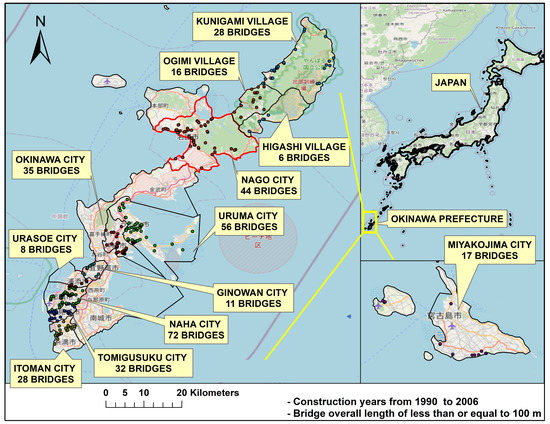
Figure 1.
Road bridges in Nago City, 8 major cities, and 3 villages in Okinawa Prefecture built between 1990 and 2006. Each bridge’s overall length ≤ 100 m.
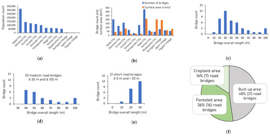
Figure 2.
Nago City, 8 major cities and 3 villages in Okinawa Prefecture. (a) Population for Nago City, 8 major cities and 3 villages in Okinawa Prefecture. (b) Road bridges and surface area for Nago City, 8 major cities, and 3 villages in Okinawa Prefecture. (c) Distribution of all 44 road bridges in Nago City of each bridge’s overall length ≤ 100 m. (d) Total of 23 medium road bridges with each bridge’s overall length between 30 m and 100 m. (e) Total of 21 short road bridges with each bridge’s overall length less than 30 m. (f) 44 road bridges in Nago City with each bridge’s overall ≤ 100 m.
The 330 road bridges in Nago City were filtered out of a total of about 700,000 road bridges in Japan. The 44 road bridges were filtered out of 330 road bridges based on construction year between 1990 and 2006 and each bridge’s overall length ≤ 100 m. The 44 road bridges were classified by surface cover type, which resulted in 21 road bridges in built-up areas, 16 in forested areas, and 7 in cropland areas, as shown in Figure 2f. Bridges were also classified by each bridge’s overall length, which resulted in 23 medium road bridges and 21 short bridges, as shown in Figure 2d and Figure 2e, respectively.
2.2. Landsat Mission
The Landsat mission is the longest-running space-based record of the Earth’s surface and atmosphere [14]. The mission is managed by both the National Aeronautics and Space Administration (NASA) and the United States Geological Survey (USGS). The goal of the mission is to monitor, manage, and understand the Earth’s resources that are necessary for sustaining human life and other living organisms. The mission consists of 8 successful operational Earth observation satellites that use remote sensors to collect data and images of our planet, as well as 1 failed satellite mission, as shown in Figure 3.
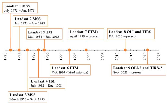
Figure 3.
The Landsat mission began in 1972, and Landsat 5 TM was used for this study. The following sensors are mounted on the Landsat satellites: MSS—Multispectral Scanner System; TM—Thematic Mapper; ETM—Enhanced Thematic Mapper; ETM+—Enhanced Thematic Mapper Plus; OLI—Operational Imager, OLI-2—Operational Imager 2; TIRS—Thermal Infrared Sensor; and TIRS-2—Thermal Infrared Sensor 2.
In the current study, the Landsat 5 Thematic Mapper was used to analyze data in Google Earth Engine.
2.3. Spectral Bands and Indices
Spectral bands in remote sensing are parts of the electromagnetic spectrum from visible radiation to optical and infrared radiation to microwave radiation that are used by various sensors to collect information from the Earth [15]. In the Landsat 5 Thematic Mapper (TM), there are 3 visible bands, 3 infrared bands, and 1 thermal infrared band, as shown in Table 1.

Table 1.
Band characteristics for Landsat 5 Thematic Mapper.
A spectral index in remote sensing is a function of two or more spectral bands of an image per pixel, as shown in Table 2. Indices are used to enhance the observation of Earth’s features such as vegetation, water, and soil, to distinguish one feature from other features in an image and to model, predict, or infer surface processes [16]. For example, the normalized difference vegetation index (NDVI) is a function of the near-infrared (NIR) band and the visible red band, expressed mathematically as NDVI = (NIR − red)/(NIR + red), and is used as an indicator of healthy vegetation [17,18]. Additionally, normalized difference water index 2 (NDWI_2) is a function of NIR and shortwave infrared 2 (SWIR2), mathematically expressed as NDWI_2 = (NIR − SWIR2)/(NIR + SWIR2), and is used as an indicator of seasonal water dynamics in wetlands [19]. Various indices have been explored in the past, some of which are listed in Table 2, and have been used in various fields such as agriculture, water resource management, and others.
In the current study, bands 1 to 5 and band 7 in Landsat 5 TM were used to analyze data in Google Earth Engine.
2.4. Data Collection and Analysis
The United States Geological Survey (USGS) produces Landsat data in three tiers for each satellite: Tier 1, Tier 2, and Real-Time (RT) [20]. Tier 1 data meet geometric and radiometric quality requirements; Tier 2 data do not meet Tier 1 quality standards; and RT data have not yet been assessed. Based on quality and other factors, the collected data are classified into Collection 1—Level 1, Collection 1—Level 2, Collection 2—Level 1, and Collection 2—Level 2 [20,21]. The data are then processed into raw or digital numbers (DNs), top of atmosphere (ToA), and surface reflectance (SR). DN represent scaled and calibrated sensor radiance, ToA represents calibrated reflectance, and SR represents atmospheric-corrected reflectance.
In the current study, 836 image pixels were collected and analyzed using Google Earth Engine. The current study consists of both Technique 1 and Technique 2, as shown in Figure 4b, and the characteristics of the current method are shown in Table 3. The data type used was Landsat 5 Thematic Mapper, SR—Level 2—Collection 2—Tier 1. The 836 image pixels were calculated as follows: 19 pixels per bridge × 44 road bridges × 1 Landsat satellite × 1 index = 836 image pixels. The 44 road bridges are shown in Table 4 and Figure 5. The applied 12 indices are shown in Figure 6 and Figure A5, for Kuroyama road bridge, and Kamiyama road bridge, respectively. The pixel satellite images for Kuroyama road bridge and Kamiyama road bridge are shown in Figure 7b and Figure A1b, respectively.
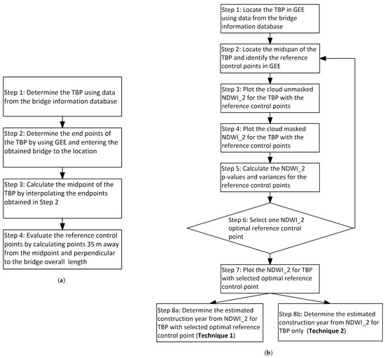
Figure 4.
Method flowchart for the previous work and current work. In the current method, Technique 1 uses both the target bridge point (TBP) and a selected optimal reference control point, while Technique 2 uses only the TBP to determine the estimated construction year. The previous method uses both the TBP and two reference control points to determine the estimated construction year. GEE is Google Earth Engine, and NDWI_2 is the normalized difference water index 2. (a) Method flowchart for the previous work [4]. (b) Method flowchart for the current work consists of both Technique 1 and Technique 2.
Table 3.
Differences between the previous method and the current method.
Table 4.
Characteristics and STARS results for all 44 road bridges.
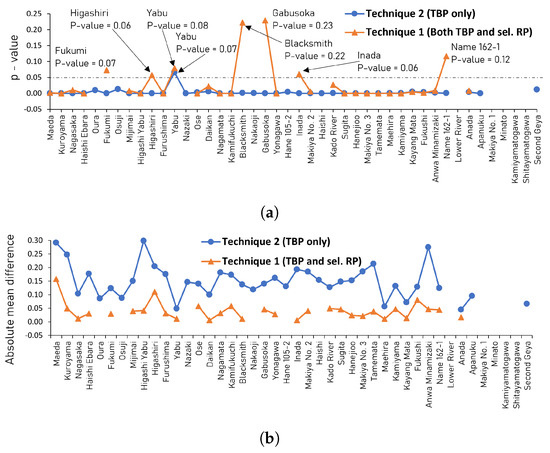
Figure 5.
The p-values and absolute mean differences for Technique 1 and Technique 2. TBP is target bridge point, and sel. RP is a selected optimum reference control point. (a) The p-values for Technique 1 and Technique 2. (b) The absolute mean differences for Technique 1 and Technique 2.
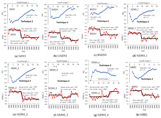
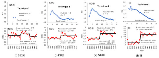
Figure 6.
GEE and STARS results for Kuroyama TBP by analyzing the 12 indices. GEE is Google Earth Engine, and STARS is a sequential t-test analysis of regime shift. The blue dots represent the absolute maximum values of regime index shift (RSI) against the cutoff length l. The red dots represent the target bridge point (TBP) only. The black line is the final optimal mean difference of the TBP data, which determines the estimated construction year. The 12 indices are presented in Table 2. Actual constr. year is actual construction year, est. constr. year is estimated construction year, and abs. mean diff. is absolute mean difference.
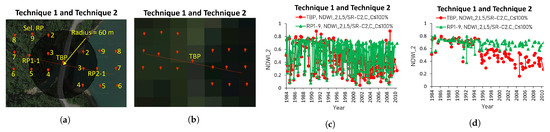
Figure 7.
Kuroyama target bridge point (TBP) and the 18 reference control points are both shown in (a,b), and Kuroyama TBP and a selected optimal reference control point (sel. RP) are shown in both (c,d). RP1-9 is a selected optimal reference control point. All four figures are used for both Technique 1 and Technique 2 in the current method. (a) Google Earth Engine image. (b) Satellite image. (c) Before cloud masking at 100% cloud cover, the trend for TBP and RP1-9 was not clear due to the presence of noise data. (d) After cloud masking at 100% cloud cover, the trend for TBP and RP1-9 was clear due to the decrease in noise data.
Table 2.
Indices attempted in the study.
Table 2.
Indices attempted in the study.
| Notation | Index Name | Formula | Application |
|---|---|---|---|
| NDVI | Normalized difference vegetation index | The study in [17] is one of the earliest papers on the use of the NDVI. The study used NDVI using Landsat 1 data to monitor and measure vegetation conditions over wide regions. Other applications include estimating crop yields, dry biomass, and changes in surface conditions [18]. | |
| GNDVI | Green normalized difference vegetation index | According to the study in [22], the difference between the NDVI and GNDVI is that the latter is more chlorophyll sensitive. If you arrange the bands in GNDVI so that the index is (green − NIR)/(green + NIR), you obtain a different index; the normalized difference water index (NDWI) is an indicator of water resources [23]. | |
| BNDVI | Blue normalized difference vegetation index | BNDVI performs the same task as the NDVI and GNDVI. The only drawback is that the blue band is easily affected by the atmosphere due to its relatively short wavelength and the resulting high relative scattering effects [24]. | |
| NDMI_1 | Normalized difference water index 1 | NDWI_1 easily maps liquid water in vegetation and is less affected by scattering effects than the NDVI [25]. | |
| NDWI_2 | Normalized difference water index 2 | The index is a good indicator of the water dynamics of seasonal wetlands [19]. | |
| NDWI_3 | Normalized difference water index 3 | The index is an indicator of open water bodies [26] but is no better than the NDWI_4 [27]. | |
| NDWI_4 | Normalized difference water index 4 | The index in [27] is a good indicator of open water features, and it suppresses vegetation, soil, and the built environment noise; it is better than the NDWI in [23]. The index also serves as an indicator of snow cover [28], which is also called the normalized difference snow index. | |
| NBR2 | Normalized burn ratio 2 | The index is an indicator of burned areas and also measures the severity of burned areas [29]. | |
| NDSI | Normalized difference soil index | The index enhances the soil information [30]. | |
| DBSI | Dry bare-soil index | The index maps built-up and bare areas in a dry climate [31]. | |
| NDBI | Normalized difference built-up index | The index maps urban built-up areas and, in some cases, barren, wooded, and agricultural areas [32]. | |
| BI | Built-up index | The index maps only the built-up and barren areas [33]. |
Note: Using Landsat 5 Thematic Mapper in Google Earth Engine, the 12 indices, which include normalized difference water index 2 (NDWI_2), were analyzed at two road bridges (Kuroyama and Kamiyama). The results for all 12 indices were accurate with a cutoff length 9, an absolute error ≤ 5, and statistically significant with p-values < 0.05, and the trends for all 12 indices were clear. In this study, the NDWI_2 was adopted and used to analyze all 44 road bridges. In the future, the other indices can be analyzed and compared along with the NDWI_2 to determine the most accurate index using Technique 2.
2.5. Cloud Masking and Cloud Shadow Masking
Cloud masking and cloud shadow masking are filtering techniques used in remote sensing to remove pixels contaminated with clouds and cloud shadows. Cloud masking technique uses the difference between the reflectance of the clear images and the reflectance of the cloud contaminated images to detect the clouds. The cloud shadow masking technique uses the difference between the reflectance of the clear images and the reflectance of the cloud shadow contaminated images to detect the cloud shadows. Both cloud masking and cloud shadow masking reduce the errors caused by erroneous mapping, improve the visibility, and, thus, increase the reflectivity of the Earth’s surface and objects on the Earth’s surface [34,35].
In the current study, the collected Landsat 5 Thematic Mapper (TM) data were cloud masked in Google Earth Engine using a Google Earth Engine open source code, and a cloud cover of 30% was used. Plots of Kuroyama road bridge and Kamiyama road bridge, before and after cloud masking at 100% cloud cover, are shown in Figure 7c and Figure 7d, as well as Figure A1c and Figure A1d, respectively. Due to noise in the data, the trends were not clear. Landsat satellites collect data every 16 days, so the Landsat 5 TM should have about 600 data points per bridge from 1984 to 2010. Before cloud masking at 100% cloud cover, about 52% of the data points were collected, and after cloud masking at 100% cloud cover, about 21% of the data points were collected. The 100% cloud cover was reduced to 30% cloud cover, and about 14% of the data points were collected. At 30% cloud cover and after the data points were averaged annually, the trends were clear, as shown in Figure 8a and Figure A2a for Kuroyama road bridge and Kamiyama road bridge, respectively. Both cloud masking and cloud cover control reduce noise in the data, and annual averaging of the data reduces seasonal variations.
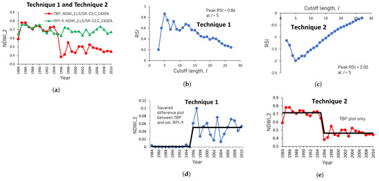
Figure 8.
Technique 1 and Technique 2 results for Kuroyama road bridge. RSI is regime shift index, and GEE is Google Earth Engine. The blue dots in (b,c) represent the absolute maximum values of regime index shift (RSI) against the cutoff length l. The blue diamonds in (d) represent the squared difference between the target bridge point (TBP) and a selected optimal reference control point (RP1-9). The red dots in (e) represent the TBP only. The black lines in (d,e) are the final optimal mean differences, which determines the estimated construction year. (a) GEE results for Technique 1 and Technique 2. (b) Peak RSI for Technique 1. (c) Peak RSI for Technique 2. (d) Estimated construction year for Technique 1 is 1996, while the actual construction year is 1997. (e) Estimated construction year for Technique 2 is 1996, while the actual construction year is 1997.
2.6. Sequential t-Test Analysis of Regime Shift (STARS) Method
Sequential t-test analysis of regime shift (STARS) is a statistical method for detecting change points in time series data [36,37,38,39]. The method identifies the point in time when the mean of the time series data changes significantly. The change in the mean can be either a single change or multiple changes within a time series. The STARS method is based on the statistical technique of the Student’s t-test, and [38,39] describes the algorithm. The algorithm was coded in Visual Basic for use in a Microsoft Excel add-in and is available for download as freeware at www.BeringClimate.noaa.gov. The STARS method can be set to detect regimes with specific time scales and magnitudes. The inputs to the STARS Microsoft Excel add-in were the cutoff length l, the significance level , and the Huber weight parameter H. The cutoff length l and the significance level are the main inputs that affect the magnitude of the regime shifts [40].
The STARS method uses Equations (1)–(6) to analyze and determine the regime shift of the mean in the time series data.
where is the absolute difference between the mean of the current and new regime, is the mean of the current regime, is the mean of the new regime, l is the cutoff length, is the degree of freedom, is the significance level, and t is the value of the t-distribution, which is a function of and . It is assumed that the variance at any given value of l is the same and equal to the average variance for the running l year intervals in the time series . Therefore, for the entire session of the time series at each given value of l. At the current time , the mean value of the new regime is unknown, but it is known that it should be equal or greater than the critical level if the shift is upward or equal or less than if the shift is downward, where
If the current value is greater than or less than , the current time is marked as a potential change point c, and subsequent data are used to reject or accept this hypothesis. The null hypothesis states that “there is an existence of a regime shift”. The test has three possible outcomes: accept , reject , or keep testing. The testing process consists of calculating the so-called regime shift index that represents a cumulative sum of the normalized anomalies relative to the critical level :
If at any time during the testing period from to , the index turns negative in the case of or positive in the case of , the null hypothesis about the existence of a regime shift at the current time is rejected, and the value is included in the current regime . Otherwise, the time is declared a change point c.
In the current study, the STARS method was used to interpret the estimated construction year from NDWI for both techniques. The inputs, cutoff length l = 2 to l = 27, significance level = 0.05, and Huber’s weight parameter H = 1 were used. The numbers 2 to 27 were used for l, because the total number of data points in the time series data was 27. The number 1 could not be used, because it had no value of t in the t-distribution because the . From the cutoff length l = 2 to l = 27, the optimal absolute maximum regime shift index was determined and thus used to identify the estimated construction year. There are three possible outcomes of the STARS method test: fail to reject the null hypothesis , reject the null hypothesis , or keep testing. The null hypothesis is a regime shift in the time series data.
2.7. Flowchart and Description of the Current Method
The flowchart for the current method is shown in Figure 4b. The current method consists of both Technique 1 and Technique 2. Technique 1 uses both the TBP and a selected optimal reference control point, while Technique 2 only uses the TBP to determine the estimated construction year of the road bridge. Japan has about 700,000 road bridges. From about 700,000 road bridges, 330 road bridges in Nago City were filtered out. Nago City is located in the northern part of Okinawa Prefecture. From 330 road bridges, 44 road bridges were filtered out based on each bridge’s overall length between 0 m and 100 m and construction year between 1990 and 2006, as shown in Table 4.
In Step 1 and Step 2, we used Google Earth Engine (GEE) and global positioning system (GPS) coordinates, from the Japan bridge database [13] to locate the midspan of the bridge’s overall length for all 44 road bridges, which we called the target bridge point (TBP). After we located the TBP in Google Earth Engine (GEE), the new GPS coordinates at the midspan were collected and entered in GEE. A perpendicular line to the bridge’s overall length was drawn 60 m from the TBP, and 18 reference control points were established, with 9 points on each side of the TBP. Each reference control point and TBP occupied an independent and unique image pixel with a spatial resolution of 30 m, as shown in Figure 7a and Figure 7b, as well as Figure A1a and Figure A1b, for Kuroyama road bridge and Kamiyama road bridge, respectively. The 60 m distance was chosen, because it had less interference from the TBP image pixel. The GPS coordinates for the 18 reference control points were collected and entered into GEE. GEE is a cloud computing program for geospatial data analysis and visualization [41].
In Step 3, we analyzed the cloud unmasked data at 100% cloud cover in GEE at the TBP and 18 reference control points, as shown in Figure 7c and Figure A1c for Kuroyama road bridge and Kamiyama road bridge, respectively. Landsat 5 Thematic Mapper (TM) was used for the analysis. Cloud unmasked data are data points whose pixels are contaminated with clouds and cloud shadows and, therefore, obscure the visibility of the surface cover due to the noise in the data.
In Step 4, we used GEE to cloud mask the data at 100% cloud cover at the TBP and 18 reference control points, as shown in Figure 7d and Figure A1d for Kuroyama road bridge and Kamiyama road bridge, respectively. Landsat 5 Thematic Mapper (TM) was used for the analysis. The cloud cover was reduced from 100% to 30%, and the data were averaged annually, as shown in Figure 8a and Figure A2a for Kuroyama road bridge and Kamiyama road bridge, respectively. Both cloud masking and cloud cover control reduce noise in the data, and annual averaging of the data reduces seasonal variations.
In Step 5, we calculated the p-values and variances at the TBP and 18 reference control points. This step was performed to check the normality and variation of the data points at the TBP and the reference control points. Homogeneity of the data is assumed when the variance is minimal and the p-value > 0.05.
In Step 6 and Step 7, we selected an optimal reference control point from the 18 reference control points. The reference control point with the lowest minimum variance and p-value > 0.05 was considered an optimal reference control point. If two or more reference points had the same variance values and p-value > 0.05, the reference control point farthest from the TBP was selected as the optimal point, because it was considered to be least affected by the interference from the TBP. The TBP and a selected optimal reference control point were plotted together, as shown in Figure 8a and Figure A2a for Kuroyama road bridge and Kamiyama road bridge, respectively.
In Step 8a, Technique 1, which uses both the TBP and a selected optimal reference control point, was used to determine the estimated construction year. The sequential t-test analysis of regime shift (STARS) method [40] was used to interpret the estimated construction year from NDWI for the squared difference between TBP and a selected optimal reference control point, as shown in Figure 8b and Figure 8d, as well as Figure A2b and Figure A2d, for Kuroyama road bridge and Kamiyama road bridge, respectively.
In Step 8b, Technique 2, which uses only the TBP, was used to determine the estimated construction year. The STARS method [40] was used to interpret the estimated construction year from NDWI for the TBP only, as shown in Figure 8c and Figure 8e, as well as Figure A2c and Figure A2e, for Kuroyama road bridge and Kamiyama road bridge, respectively.
2.8. Comparison of Methods between the Previous Method and the Current Method
The current method is an improvement of the previous method [4]. The current method consists of both Technique 1 and Technique 2. Technique 1 uses both the target bridge point (TBP) and a selected optimal reference control point, while Technique 2 uses only the TBP, to determine the estimated construction year of the road bridge. The previous method uses both the TBP and two reference control points to determine the estimated construction year. The flowchart for the previous method is shown in Figure 4a, and that for the current method is shown in Figure 4b. The summary of the differences between the previous method and the current method are presented in Table 3.
Step 1 of the previous method in Figure 4a describes how the location of the TBP was determined using data from the bridge information database, which was similar to Step 1 of the current method in Figure 4b. Step 2 of the previous method in Figure 4a describes how the TBP endpoints were determined in Google Earth Engine (GEE), and this Step was included in Step 2 of the current method, as shown in Figure 4b. Step 3 of the previous method in Figure 4a describes how the midspan of the TBP was determined, and this Step was also included in Step 2 of the current method, as shown in Figure 4b. Finally, Step 4 of the previous method describes how the two reference control points were established on either side of the TBP at 35 m from the TBP perpendicular to each bridge’s overall length. This step was included in Step 2 of the current method, as shown in Figure 4b, where 60 m from the TBP and perpendicular to each bridge’s overall length was used, because it had less interference from the TBP.
The current method in Figure 4b differs from the previous method in Figure 4a in that the current method (a) performs cloud masking of the data, (b) reduces cloud cover from 100% to 30%, (c) averages the data annually, (d) selects an optimal reference control point with the lowest minimum variance and p-value > 0.05, and (e) uses the sequential t-test analysis of the regime shift method to interpret the estimated construction year from the NDWI. Both cloud masking and cloud cover control reduce noise in the data, and annual averaging of the data reduces seasonal variations. Homogeneity of the data is assumed when the variance is minimal and p-value is >0.05.
3. Results
A total of 836 image pixels were analyzed in the Google Earth Engine, which were calculated as follows: 19 pixels per bridge × 44 road bridges in Nago City × 1 Landsat satellite × 1 index = 836 image pixels. Each analyzed road bridge was unique and had its own characteristics and behaviors. The Landsat satellite collects data on the Earth’s surface every 16 days per image pixel. For the period from 1984 to 2010, the Landsat 5 Thematic Mapper is expected to collect about 600 data points per image pixel. The average total percentage of data points collected in the Nago City for each road bridge in Landsat 5 TM was about 52% for cloud unmasked data at 100% cloud cover, about 21% for cloud masked data at 100% cloud cover, and about 14% for cloud masked data at 30% cloud cover. Summaries of the results, p-values, and absolute mean differences for all 44 road bridges are presented in Table 4, Figure 5a and Figure 5b, respectively.
3.1. Sensitivity Analysis for Sequential t-Test Analysis of Regime Shift (STARS) Method
The sequential t-test analysis of the regime shift (STARS) method was used to interpret the estimated construction year from the NDWI_2 for both Technique 1 and Technique 2. Technique 1 uses both the target bridge point (TBP) and a selected optimal reference control point, while Technique 2 uses only the TBP. The STARS method has three inputs: the
Huber’s weight parameter H, the significance level , and the cutoff length l. The values of the Huber’s weight parameter at H = 1, 3, and 6 were tested, and the results obtained were the same, or the differences were negligible. A similar trend was observed by [42]; therefore, H = 1 was assumed for all road bridges. The inputs cutoff length l = 2 to l = 27 and significance level = 0.05 were used for all road bridges. The numbers 2 to 27 were used for l because the total number of data points in the time series was 27. The number 1 could not be used because it had no value of t in the t-distribution, since . From the cutoff length l = 2 to l = 27, the optimal absolute maximum regime shift index was determined and, thus, used to identify the estimated construction year. A time series with a downward shift results in a negative , and an upward shift results in a positive . An example of the cutoff length l and optimal absolute maximum regime shift index results are shown in Figure 8b and Figure 8c, as well as Figure A2b and Figure A2c for the Kuroyama road bridge and Kamiyama road bridge, respectively.
3.2. Analysis and Results of 12 Indices at 2 Road Bridges
Technique 2 was used in the analysis of 12 indices. Technique 2 uses only the target bridge point (TBP) to determine the estimated construction year of the road bridge. This analysis was performed to gain an understanding of the trends of the 12 indices in Table 2.
Two road bridges, the Kuroyama road bridge and Kamiyama road bridge, were analyzed using the 12 indices at the TBP. The trends and results for the two road bridges are shown in Figure 6 and Figure A5 for the Kuroyama road bridge and Kamiyama road bridge, respectively. The absolute errors between the actual and estimated construction year were comparable and ranged from 0 to 5 years. The cutoff length was 9, and the p-value was < 0.05 for all 12 indices. However, no results were recorded for the normalized difference water index 3 (NDWI_3) and the normalized difference soil index (NDSI), as shown in Figure A5f,i for the Kamiyama road bridge.
In this study, the normalized difference water index 2 (NDWI_2) was used to analyze all 44 road bridges. In the future, the other indices can be analyzed and compared along with the NDWI_2 to determine the most accurate index.
3.3. Analysis and Results of Normalized Difference Water Index 2 at All 44 Road Bridges
Technique 1 and Technique 2 were used in the analysis of all 44 road bridges. Technique 1 uses both the target bridge point (TBP) and a selected optimal reference control point, while Technique 2 only uses the TBP, to determine the estimated construction year of the road bridge.
The 44 road bridges were analyzed using the normalized difference water index 2 (NDWI). The summarized results in terms of the p-values and absolute mean differences for all 44 road bridges are shown in Table 4, Figure 5a and Figure 5b, respectively. The absolute errors between the actual and estimated construction year ranged from 0 to 17 years, the cutoff length 25, and the p-value ≤ 0.23.
For brevity, only the results for three road bridges are presented. The three road bridges are the Kuroyama, Kamiyama, and Shitayamatogawa. The trends and results for the Kuroyama road bridge, Kamiyama road bridge, and Shitayamatogawa road bridge are shown in Figure 7 and Figure 8, Figure A1 and Figure A2, and Figure A3 and Figure A4, respectively.
The Kuroyama road bridge is shown in both Figure 7 and Figure 8. The Google image and satellite image of the road bridge are shown in Figure 7a and Figure 7b, respectively. The trends in Figure 7c were not clear because of noise in the data that were not cloud-masked. After cloud masking, the trends in Figure 7d were clear, because the noise in the data was reduced. The trends were even clearer when cloud cover was reduced from 100% to 30%, and the data were averaged annually, as shown in Figure 8a. Both cloud masking and cloud cover control reduce noise in the data, and annual averaging of the data reduces seasonal variations. The results for Technique 1 are shown in Figure 8b,d, and the results for Technique 2 are shown in Figure 8c,e. Both Technique 1 and Technique 2 recorded an absolute error between the actual and estimated construction year of 1 year; the cutoff length 5, and the p-value < 0.05, as shown in Figure 5a and Figure 8d,e.
Similar trends and results were observed for the Kamiyama road bridge. Figure A1, Figure A2, Figure A3 and Figure A4 show the results for the Shitayamatogawa road bridge. Using the STARS method, no regime shift was detected for the Shitayamatogawa road bridge for both Technique 1 and Technique 2, as shown in Figure A4b, and Figure A4c, respectively. The results for the rest of the road bridges for both techniques are shown in Table 4 and Figure 5a,b.
3.4. Comparison of Results between the Previous Method and the Current Method
The previous method used both the TBP and the two reference control points to determine the estimated construction year of the road bridge. The current method consists of both Technique 1 and Technique 2. Technique 1 uses both the target bridge point (TBP) and a selected optimal reference control point, while Technique 2 only uses the TBP, to determine the the estimated construction year of the road bridge.
In the previous method, the data were contaminated with noise, because there was no cloud masking or cloud cover control; therefore, the trends were not clear. Additionally, no technique was used to interpret the estimated constructed year from the NDWI. Figure 9a shows the trends and results for the previous method compared to the trends and results for the current method in Figure 9b. The result for the current method in Figure 9b was clear and was further analyzed using the STARS method for both Technique 1 and Technique 2, as shown in Figure 8d and Figure 8e, respectively. Table 5 presents a summary of the comparative advantages between the results of the previous method and the current method.
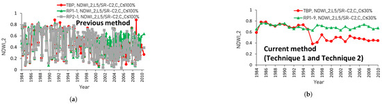
Figure 9.
Comparison of results for Kuroyama road bridge between the previous method and current method. (a) Kuroyama road bridge in the previous method [4]. Neither cloud masking nor cloud cover control were performed. The actual construction year was 1997, and the estimated construction year was unclear due to noise in the data. (b) Kuroyama road bridge in the current method. Both cloud masking and cloud cover control were performed. The actual construction year was 1997, and the estimated construction year was 1996 for both Technique 1 and Technique 2, as shown in Figure 8d and Figure 8e, respectively.
Table 5.
Comparative advantages between the results of the previous method and current method.
4. Discussion
We found that the mean differences for all 44 road bridges in Table 4 were statistically significant with p-values < 0.05, except for seven road bridges in Technique 1 and one road bridge in Technique 2, as shown in Figure 5a. The absolute mean differences for Technique 1 and Technique 2 are shown in Figure 5b. Technique 1 uses both the target bridge point (TBP) and a selected optimal reference control point, while Technique 2 uses only the TBP, to determine the estimated construction year of the road bridge.
Table 6 shows the summary of the results of the correlation analysis. The correlation analysis yielded an = 0.24 and an = 0.33, as well as an average deviation of S = 5.81 years and S = 4.08 years for Technique 1 and Technique 2, respectively, as shown in Figure 10a and Figure 10b, respectively. The results suggest that Technique 2 is more accurate and provides a better estimate than Technique 1, but the values were low. One of the possible explanations that may have contributed to low values, as indicated by the gap between the actual and estimated construction year in Figure 10, is that the planned construction year recorded in the database may not have corresponded to the actual construction year due to construction delays [4].
Table 6.
Summary of the coefficient of determination for all 44 road bridges in Table 4 according to overall length and surface cover.
Table 6.
Summary of the coefficient of determination for all 44 road bridges in Table 4 according to overall length and surface cover.
| Coefficient of Determination | ||
|---|---|---|
| Technique 1 | Technique 2 | |
| 44 road bridges in Figure 10a, and Figure 10b, resp. | 0.24 | 0.33 |
| 23 road bridges in forested and cropland areas Figure 11a, and Figure 11b, resp. | 0.23 | 0.42 |
| 21 road bridges in the built-up areas Figure 11c, and Figure 11d, resp. | 0.09 | 0.05 |
| 23 medium road bridges in Figure 12a, and Figure 12b, resp. | 0.09 | 0.41 |
| 21 short road bridges Figure 12c, and Figure 12d, resp. | 0.40 | 0.20 |
| Mean value | 0.21 | 0.28 |
Note: Resp. is respectively. Technique 1 uses both the target bridge point (TBP) and a selected optimal reference control point, while Technique 2 uses only the TBP, to determine the estimated construction year of the road bridge.

Figure 10.
Correlation results of the actual construction year against estimated construction year. S is standard error of the regression, which represents the average distance that the observed values fall from the regression line. (a) Technique 1 correlation results for all 44 road bridges. (b) Technique 2 correlation results for all 44 road bridges.


Figure 11.
Correlation results of the actual construction year against estimated construction year. S is the standard error of the regression, which represents the average distance that the observed values fall from the regression line. (a) Technique 1 correlation results for 23 road bridges in the forested and cropland areas. (b) Technique 2 correlation results for 23 road bridges in the forested and cropland areas. (c) Technique 1 correlation results for 21 road bridges in the built-up areas. (d) Technique 2 correlation results for 21 road bridges in the built-up areas.


Figure 12.
Correlation results of the actual construction year against estimated construction year. S is the standard error of the regression, which represents the average distance that the observed values fall from the regression line. (a) Technique 1 correlation results for 23 medium road bridges in Figure 2d. (b) Technique 2 correlation results for 23 medium road bridges in Figure 2d. (c) Technique 1 correlation results for 21 short road bridges in Figure 2e. (d) Technique 2 correlation results for 21 short road bridges in Figure 2e.


The 44 road bridges were classified and analyzed, for both Technique 1 and Technique 2, according to each bridge’s overall length and surface cover type, as shown in Figure 2 and Table 6. For Technique 1, an = 0.40 was determined for the short road bridges, as shown in Figure 12c, but the number of data points was small. For Technique 2, an = 0.41 was higher for medium road bridges than an = 0.20 for short road bridges, and an = 0.42 was higher for road bridges in forested and cropland areas than an = 0.05 for road bridges in built-up areas, as shown in Table 6.
The results suggest that a greater overall length of road bridges and road bridges in forested areas contributed to accuracy. One of the possible explanations is that a road bridge with a greater overall length and a reasonable road width has a large surface area that results in a higher reflectance value, provided that the reflectance is minimally attenuated by scattering and absorption effects, and the image pixel is sufficiently covered by the road bridge surface. No analysis of the relationship between road width and accuracy was performed in this study. The normalized difference water index 2 (NDWI_2) is a function of near-infrared band (NIR) and shortwave infrared band 2 (SWIR2) values. Green healthy vegetation has a higher reflectance value in the NIR than in the SWIR2, and green healthy vegetation also has a higher reflectance value than asphalt or concrete surfaces in the NIR [43]. Therefore, the reflectance is expected to be higher before the bridge is built, assuming that the original surface cover was green healthy vegetation. After the road bridge is built, the reflectance decreases significantly, which in turn increases the mean difference between the current and new regimes in the sequential t-test analysis of the regime shift method assuming that the reflectance is minimally attenuated due to scattering and absorption effects.
The increase in the regime shift index had an insignificant effect on the absolute error between the actual and estimated construction year, as shown in Figure 13a,b. However, as the cutoff length l increased, the absolute error between the actual and estimated construction year increased, as shown in Figure 13c,d. The degree of freedom also increases as the cutoff length l increased, thus leading to a decrease in the statistically significant difference between the means of the two successive regimes [38,39], as shown in Equations (1)–(3). To increase the accuracy of the estimated construction year, we may consider setting the upper limit of the cutoff length l to 12 from Figure 13d. Based on the clustered results with minimum absolute errors in Figure 13d, 12 was selected as the working limit from the linear regression analysis between the cutoff length l and the absolute error between the actual and estimated construction year for Technique 2.
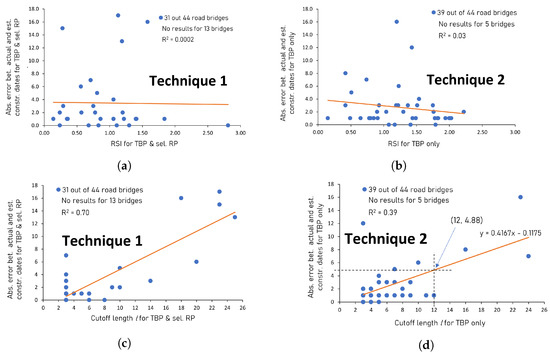
Figure 13.
Correlation results of the and cutoff length l versus absolute error between the actual and estimated construction year. Abs. is absolute, bet. is between, constr. is construction, est. is estimated, sel. RP is the optimum selected reference control point, RSI is the regime shift index, TBP is the target bridge point, and S is the standard error of the regression, which represents the average distance that the observed values fall from the regression line. (a) Technique 1 results for versus absolute error of all 44 road bridges. (b) Technique 2 results for versus absolute error of all 44 road bridges. (c) Technique 1 results for cutoff length l versus absolute error of all 44 road bridges. (d) Technique 2 results for cutoff length l versus absolute error of all 44 road bridges.
The 12 indices in Table 2 were analyzed at the two road bridges (Kuroyama, and Kamiyama), as shown in Figure 6 and Figure A5. Additionally, the following results were obtained: cutoff length ≤ 9, absolute error ≤ 5, and p-values < 0.05. Using the adopted measure of accuracy, 12, the results for the 12 indices were accurate and statistically significant. However, for the two indices, the normalized difference water index 3 and normalized difference soil index, no regime shifts were detected at the Kamiyama road bridge, as shown in Figure A5f,i. The lack of results could be due to seasonal variations and inadequate reflectance.
Technique 1, which uses both the TBP and a selected optimal reference control point to determine the estimated construction year, found inaccurate and statistically insignificant results for five road bridges, statistically insignificant results for two road bridges, and no results for thirteen road bridges. The five road bridges with inaccurate and statistically insignificant results were the Fukumi, Yabu, Blacksmith, Gabusoka, and Inada, and the two road bridges with statistically insignificant results were the Name 162-1 and Higashiri, which are collectively shown in Figure 5a, Figure 10a, Figure 11a,c and Figure 12a,c. Additionally, the thirteen road bridges without results were the Osuji, Second Geya, Kamiyamatogawa, Shitayamatogawa, Haishi, Hane 105-2, Oura, Nazaki, Nakaoji, Apanuku, Lower River, Makiya No. 1, and Minato, as shown in Table 4. The upper limits 12, and p-value ≤ 0.05 were used as measures of accurate results and statistically significant results, respectively. The Fukumi, Yabu, Blacksmith, Gabusoka, and Inada all recorded 12 and a p-values > 0.05, and the Name 162-1 and Higashiri both recorded p-values > 0.05, as shown in Figure 5a and Table 4. The inaccurate results and the lack of results for the road bridges could be due to seasonal variations and inadequate reflectance. Excessive seasonal variations were observed at the Fukumi road bridge, which may have contributed to inaccurate results. Excessive seasonal variation at all selected optimal reference control points for five road bridges with inaccurate results may have also contributed to the inaccurate results. The Haishi Ebara road bridge was found to have l = 14 > 12, absolute error = 3, and p-value < 0.05. The absolute error was low, but l was high, which could be due to a small mean difference between successive regimes, as shown in Table 4 and Figure 5.
Technique 2, which uses only TBP to determine the estimated construction year, found inaccurate results for three road bridges, a statistically insignificant result for one road bridge, and no result for five road bridges. The three road bridges with inaccurate results were the Fukumi, Kayang Mata, and Maehira, and the one road bridge with statistically insignificant result was the Yabu, which are collectively shown in Figure 5a, Figure 10b, Figure 11b,d and Figure 12b,d. And five road bridges without results were the Kamiyamatogawa, Shitayamatogawa, Lower River, Makiya No. 1, and Minato, as shown in Table 4. The upper limits 12 and p-value ≤ 0.05 were used as measures of accurate results and statistically significant results, respectively. The Fukumi, Kayang Mata, and Maehira all recorded 12, and the Yabu recorded a p-value > 0.05, as shown in Table 4 and Figure 5a. The inaccurate results and the lack of results for the road bridges could be due to seasonal variation and inadeqaute reflectance. All three road bridges with inaccurate results had seasonal variations that could have contributed to the inaccurate results. Of the three road bridges, the Fukumi had excessive seasonal variations. The overall lengths of both the Maehira road bridge and the Kayang Mata road bridge were less than 30 m and may have contributed to inaccurate results in the STARS method due to inadequate reflectance.
Table 5 shows the comparative advantages between the results for the previous method and the current method. The previous method used both the TBP and two reference control points to determine the estimated construction year. The current method consists of Technique 1 and Technique 2. Technique 1 uses both the TBP and a selected reference control point, while Technique 2 uses only the TBP, to determine the estimated construction year of the road bridge. Among the three methods in Table 5, Technique 2 is the better estimate.
The 44 road bridges in Table 4 were classified according to their surface cover and each bridge’s overall length for Technique 1 and Technique 2, and the summary of the results are shown in Table 6. For Technique 2, an = 0.42 was obtained for the forested and cropland areas, which was higher than the = 0.23 value for Technique 1. In the built-up areas, both Techniques recorded comparatively low values of = 0.09 and = 0.05 for Technique 1 and Technique 2, respectively. For Technique 2, an = 0.41 was obtained for medium road bridges, which was higher than the = 0.09 value for Technique 1. For Technique 1, an = 0.40 was obtained for short road bridges, which was higher than the = 0.20 value for Technique 2. The results indicate that an increase in the bridge’s overlength length, as well as forested and cropland areas, contributed to the accuracy of the results. All five road bridges in Technique 2 that did not produce results had bridge overall lengths of less than 30 m. Additionally, of the thirteen road bridges in Technique 2 that did not produce results, eight out of thirteen road bridges had bridge overall lengths of less than 30 m.
Nevertheless, the two proposed techniques have a number of limitations and challenges. Seasonal variations and inadequate reflectance at the TBP and the selected optimal reference control points are not easily controled. Neither technique can be readily applied in regions where the TBP is obscured by natural or artificial cover for extended periods. Neither technique can be readily applied in regions not covered by Landsat or related satellites, and neither technique can be readily applied in regions where Landsat or related satellite data are severely attenuated by atmospheric absorption and scattering effects.
In the future, the STARS method could be extended to automatically cycle through all values of a certain cutoff length l in the time series data and then produce an optimal peak at a given value of l. In future research, some correction factors could be determined using statistics or mathematical formulas to account for seasonal variations and inadequate reflectance at the TBP, as well as using all image pixels across the whole span of the TBP to increase reflectance. The cutoff length 12 is a working limit; therefore, in the future, there is a need to develop a robust reliability method for these proposed techniques. Finally, the generality of these two proposed techniques needs to be tested in other geographic areas.
5. Conclusions
The correlation analysis showed that increasing the cutoff length l increased the absolute error between the actual and estimated construction years. Therefore, as a measure of accuracy, the upper limit of cutoff length l was set to 12. Based on the clustered results with minimum absolute errors, 12 was selected as the working limit from the linear regression analysis between the absolute error between the actual and estimated construction year and the cutoff length l for Technique 2.
Landsat 5 Thematic Mapper (TM) in Google Earth Engine (GEE) was used for the analysis. The 12 indices, which included the normalized difference water index 2 (NDWI_2), were analyzed at two road bridges (Kuroyama and Kamiyama). The results for all 12 indices were accurate with a cutoff length 9, an absolute error ≤ 5, and statistically significant with p-values < 0.05. The trends for all 12 indices were clear. The NDWI_2 was adopted and used for the analysis of all 44 road bridges. In the future, the remaining indices can be analyzed and compared along with the NDWI_2 to determine the most accurate index using Technique 2. Sequential t-test analysis of regime shift (STARS) with a significance level of = 0.05 and cutoff lengths of l = 2 to l = 27 was used to interpret the estimated construction year from Landsat 5 TM data generated from all 12 indices.
Landsat 5 TM in GEE was used for the analysis. The NDWI_2 data were cloud masked in GEE, the cloud cover was reduced from 100% to 30% in GEE, and the data were averaged annually for both techniques. Both cloud masking and cloud cover control reduce noise in the data, and averaging the data annually reduces seasonal variations. Technique 1 uses both the target bridge point (TBP) and a selected optimal reference control point, while Technique 2 uses only the TBP, to determine the estimated construction year of the road bridge. The STARS method was used at = 0.05 and l = 2 to l = 27 to interpret the estimated construction year from Landsat 5 TM NDWI_2 data.
Both techniques successfully determined the estimated construction year, which was statistically significant with p-values < 0.05, except for seven bridges in Technique 1 and one road bridge in Technique 2. The correlation analysis of all 44 road bridges yielded an = 0.24 and an = 0.33, as well as an average deviation of S = 5.81 years and S = 4.08 years, for Technique 1 and Technique 2, respectively. The results suggest that Technique 2 is more accurate and is a better estimate than Technique 1, but the values were low. One of the possible explanations that may have contributed to low values, as indicated by the gap between the actual and estimated construction year, is that the planned construction year recorded in the database may not have corresponded to the actual construction year due to construction delays.
For Technique 1, the Haishi Ebara road bridge was found to have an l = 14 > 12, an absolute error = 3, and a p-value < 0.05. The absolute error was low, but l was high, which could be due to a small mean difference between successive regimes. The cutoff length 12 is a working limit; therefore, in the future, there is a need to develop a robust reliability method for these proposed techniques.
Some of the advantages of Technique 2 over Technique 1 are that (a) the analysis time was relatively shorter with Technique 2 than with Technique 1 and (b) Technique 2 did not use a selected optimal reference point, which in most cases negatively affected the final results due to seasonal variations.
A longer bridge’s overall length and road bridges in forested areas contribute to the accuracy of the results. One of the possible explanations is that a larger surface area corresponds to a higher reflectance, and the near-infrared in normalized difference water index 2 has a higher reflectance for green vegetation than for asphalt or concrete surface areas.
The comparative analysis indicated that the results for the previous technique were not clear when compared to the results of the current Technique 1 and Technique 2. Due to the lack of cloud masking and control of cloud cover, the data were contaminated with noise in the previous method.
The proposed techniques can be applied to detect any significant mean difference on the Earth’s surface, whether natural or man-made. The region must be covered by Landsat or related satellites, the features on the Earth’s surface must not be obscured by natural or human cover for extended periods, and the data from the Landsat or related satellites must not be severely attenuated by atmospheric absorption and scattering effects.
By using the construction year as one of the inputs for bridge management systems, bridge managers can make more informed decisions about how best to maintain and improve road bridges to ensure user safety and bridge preservation for the future.
Author Contributions
Conceptualization, B.H., K.M. and K.N.; Methodology, B.H.; Validation, B.H., K.M. and K.N.; Formal analysis, B.H.; Investigation, B.H.; Resources, B.H. and K.M.; Data curation, B.H.; Writing—original draft, B.H.; Writing—review and editing, B.H.; Supervision, K.M. and K.N. All authors have read and agreed to the published version of the manuscript.
Funding
The authors disclosed receipt of the following financial support for the research, authorship, and/or publication of this article: The research has been funded by the Japan International Cooperation Agency.
Data Availability Statement
The data that support the findings of this study are available in the public domain in Google Earth Engine at https://code.earthengine.google.com/, and the Japan National Road Facility Inspection Database at https://road-structures-map.mlit.go.jp/FacilityList.aspx, all accessed on 21 December 2022.
Acknowledgments
The authors would like to thank four anonymous reviewers for their comments that helped to improve the manuscript.
Conflicts of Interest
The authors declare no potential conflicts of interest with respect to the research, authorship, and/or publication of this article.
Abbreviations
The following abbreviations are used in this manuscript:
| NDWI_2 | Normalized Difference Water Index 2 |
| TBP | Target Bridge Point |
| GEE | Google Earth Engine |
| STARS | Sequential t-test Analysis of Regime Shift |
| Sel. RP | Selected Optimal Reference Point |
Appendix A
The appendix contains additional information on the Kamiyama road bridge, Shitayamatogawa road bridge, and the 12 indices at the Kamiyama road bridge. All the figures in the appendix have been referenced in the main document.
Figure A1: Kamiyama road bridge (before and after cloud masking).
Figure A2: Kamiyama road bridge (estimated construction year).
Figure A3: Shitayamatogawa road bridge (before and after cloud masking).
Figure A4: Shitayamatogawa road bridge (estimated construction year).
Figure A5: the 12 indices at Kamiyama road bridge.

Figure A1.
Kamiyama target bridge point (TBP) and the 18 reference control points are both shown in (a,b), and the Kamiyama TBP and a selected optimal reference control point (sel. RP) are shown in both (c,d). RP1-5 is a selected optimal reference control point. All four figures are used for both Technique 1 and Technique 2 in the current method. (a) Google Earth Engine image. (b) Satellite image. (c) Before cloud masking at 100% cloud cover, the trend for TBP and RP1-9 was not clear due to the presence of noise data. (d) After cloud masking at 100% cloud cover, the trend for TBP and RP1-9 was clear due to the decrease in noise data.


Figure A2.
Technique 1 and Technique 2 results for Kamiyama road bridge. RSI is regime shift index, and GEE is Google Earth Engine. The blue dots in (b,c) represent the absolute maximum values of regime index shift (RSI) against the cutoff length l. The blue diamonds in (d) represent the squared difference between the target bridge point (TBP) and a selected optimal reference control point (RP1-5). The red dots in (e) represent the TBP only. The black lines in (d,e) are the final optimal mean differences, which determines the estimated construction year. (a) GEE results for Technique 1 and Technique 2. (b) Peak RSI for Technique 1. (c) Peak RSI for Technique 2. (d) Estimated construction year for Technique 1 is 1992, while the actual construction year is 1993. (e) Estimated construction year for Technique 2 is 1992, while the actual construction year is 1993.


Figure A3.
Shitayamatogawa target bridge point (TBP) and the 18 reference control points are both shown in (a,b), and the Shitayamatogawa TBP and a selected optimal reference control point (sel. RP) are shown in both (c,d). RP2-5 is a selected optimal reference control point. All four figures are used for both Technique 1 and Technique 2 in the current method. (a) Google Earth Engine image. (b) Satellite image. (c) Before cloud masking at 100% cloud cover, the trend for TBP and RP1-9 was not clear due to the presence of noise data. (d) After cloud masking at 100% cloud cover, the trend for TBP and RP1-9 was clear due to the decrease in noise data.


Figure A4.
Technique 1 and Technique 2 results for Shitayamatogawa road bridge. RSI is regime shift index, and GEE is Google Earth Engine. The blue diamonds in (b) represent the squared difference between the target bridge point (TBP) and a selected optimal reference control point (RP2-5). The red dots in (c) represent the TBP only. The black lines in (b,c) are the final optimal mean differences, which determines the estimated construction year. No mean differrence was detected, therefore, no estimated construction year. (a) GEE results for Technique 1 and Technique 2. (b) Estimated construction year for Technique 1. (c) Estimated construction year for Technique 2.


Figure A5.
GEE and STARS results for Kamiyama TBP by analyzing the 12 indices.GEE is Google Earth Engine, and STARS is a sequential t-test analysis of regime shift. The blue dots represent the absolute maximum values of regime index shift (RSI) against the cutoff length l. The red dots represent the target bridge point (TBP) only. The black line is the final optimal mean difference of the TBP data, which determines the estimated construction year. The 12 indices are presented in Table 2. Actual constr. year is actual construction year, est. constr. year is estimated construction year, and abs. mean diff. is absolute mean difference.

References
- Yari, N. New model for Bridge Management System (BMS). Ph.D. Thesis, University of New Hampshire, Durham, NH, USA, 2018. [Google Scholar]
- Jiang, Y.; Sinha, K.C. Bridge Service Life Prediction Model using the Markov Chain. Transp. Res. Rec. 1989, 1223, 24–30. [Google Scholar]
- Dayarathne, W.H.R.S.; Galappaththi, G.S.; Perera, K.E.S.; Nanayakkara, S.M.A. Evaluation of the Potential for Delayed Ettringite Formation in Concrete. In Proceedings of the 19th ERU SYMPOSIUM National Engineering Conference, Moratuwa, Sri Lanka, 26 November 2013; pp. 59–66. [Google Scholar]
- Sovisoth, E.; Kuntal, V.S.; Misra, P.; Takeuchi, W.; Nagai, K. Estimation of Year of Construction of Bridges in Cambodia by Analyzing the Landsat Normalized Difference Water Index. Infrastructures 2023, 8, 77. [Google Scholar] [CrossRef]
- Soergel, U.; Thiele, A.; Gross, H.; Thoennessen, U. Extraction of bridge features from high-resolution InSAR data and optical images. In Proceedings of the 2007 Urban Remote Sensing Joint Event, Paris, France, 11–13 April 2007; pp. 1–6. [Google Scholar]
- Abraham, L.; Sasikumar, M. Analysis of satellite images for the extraction of structural features. IETE Tech. Rev. 2014, 31, 118–127. [Google Scholar] [CrossRef]
- Nettis, A.; Massimi, V.; Nutricato, R.; Nitti, D.O.; Samarelli, S.; Uva, G. Satellite-based interferometry for monitoring structural deformations of bridge portfolios. Autom. Constr. 2023, 147, 104707. [Google Scholar] [CrossRef]
- Macchiarulo, V.; Milillo, P.; Blenkinsopp, C.; Giardina, G. Monitoring deformations of infrastructure networks: A fully automated GIS integration and analysis of InSAR time-series. Struct. Health Monit. 2022, 21, 1849–1878. [Google Scholar] [CrossRef]
- Cusson, D.; Rossi, C.; Ozkan, I.F. Early warning system for the detection of unexpected bridge displacements from radar satellite data. J. Civ. Struct. Health Monit. 2021, 11, 189–204. [Google Scholar] [CrossRef]
- Aswathi, J.; Binojkumar, R.B.; Oommen, T.; Bouali, E.H.; Sajinkumar, K.S. InSAR as a tool for monitoring hydropower projects: A review. Energy Geosci. 2022, 3, 160–171. [Google Scholar] [CrossRef]
- Japan Meteorological Agency. Available online: https://www.data.jma.go.jp/gmd/cpd/longfcst/en/tourist.html (accessed on 25 January 2023).
- Nago City Population Statistics. Available online: https://www.citypopulation.de (accessed on 24 January 2023).
- National Road Facility Inspection Database for Japan. Available online: https://road-structures-map.mlit.go.jp/FacilityList.aspx (accessed on 21 December 2022).
- Landsat Science. Available online: https://landsat.gsfc.nasa.gov/ (accessed on 21 December 2022).
- Laake, A. Electromagnetic spectral bands used for remote Sensing. In Remote Sensing for Hydrocarbon Exploration; Springer: Cham, Switzerland, 2022; pp. 21–35. [Google Scholar]
- Prasad, A.D.; Ganasala, P.; Hernández-Guzmán, R.; Fathian, F. Remote sensing satellite data and spectral indices: An initial evaluation for the sustainable development of an urban area. Sustain. Water Resour. Manag. 2022, 8, 19. [Google Scholar] [CrossRef]
- Rouse, J.W., Jr.; Haas, R.H.; Schell, J.A.; Deering, D.W. Monitoring vegetation systems in the Great Plains with ERTS. NASA 1974, 1, 9. [Google Scholar]
- Tucker, C.J.; Justice, C.O.; Prince, S.D. Monitoring the grasslands of the Sahel 1984–1985. Int. J. Remote Sens. 1986, 7, 1571–1581. [Google Scholar] [CrossRef]
- Lefebvre, D.; Willm, C.; Redmond, M.; Guelmami, P. Introducing WIW for detecting the presence of water in wetlands with landsat and sentinel satellites. Remote Sens. 2019, 11, 2210. [Google Scholar] [CrossRef]
- Landsat Collection 1 vs. Collection 2 Summary U.S. Geological Survey. Available online: https://www.usgs.gov/landsat-missions/news/landsat-7-nominal-science-mission-ending (accessed on 22 December 2022).
- Landsat Full Resolution Browse Images U.S. Geological Survey. Available online: https://www.usgs.gov/landsat-missions/landsat-full-resolution-browse-images (accessed on 22 December 2022).
- Gitelson, A.A.; Kaufman, Y.J.; Merzlyak, M.N. Use of a green channel in remote sensing of global vegetation from EOS-MODIS. Remote Sens. Environ. 1996, 58, 289–298. [Google Scholar] [CrossRef]
- Mcfeeters, S.K. The use of the Normalized Difference Water Index (NDWI) in the delineation of open water features. Int. J. Remote Sens. 1996, 17, 1425–1432. [Google Scholar] [CrossRef]
- Wang, F.; Huang, J.; Tang, Y.; Wang, X. New Vegetation Index and Its Application in Estimating Leaf Area Index of Rice. Rice Sci. 2007, 14, 195–203. [Google Scholar] [CrossRef]
- Gao, B. NDWI—A normalized difference water index for remote sensing of vegetation liquid water from space. Remote Sens. Environ. 1996, 58, 257–266. [Google Scholar] [CrossRef]
- Ozelkan, E. Water body detection analysis using NDWI indices derived from landsat-8 OLI. Pol. J. Environ. Stud. 2020, 29, 1759–1769. [Google Scholar] [CrossRef] [PubMed]
- Xu, H. Modification of normalized difference water index (NDWI) to enhance open water features in remotely sensed imagery. Int. J. Remote Sens. 2006, 27, 3025–3033. [Google Scholar] [CrossRef]
- Normalized Difference Snow Index. Available online: https://www.usgs.gov/landsat-missions/normalized-difference-snow-index (accessed on 22 January 2023).
- Normalized Difference Burn Ratio 2 Index. Available online: https://www.usgs.gov/landsat-missions/landsat-normalized-burn-ratio-2 (accessed on 21 January 2023).
- Deng, Y.; Wu, C.; Li, M.; Chen, R. RNDSI: A ratio normalized difference soil index for remote sensing of urban/suburban environments. Int. J. Appl. Earth Obs. Geoinf. 2015, 39, 40–48. [Google Scholar] [CrossRef]
- Rasul, A.; Balzter, H.; Ibrahim, G.; Hameed, H.; Wheeler, J.; Adamu, B.; Ibrahim, S.; Najmaddin, P. Applying built-up and bare-soil indices from Landsat 8 to cities in dry climates. Land 2018, 7, 81. [Google Scholar] [CrossRef]
- Zha, Y.; Gao, J.; Ni, S. Use of normalized difference built-up index in automatically mapping urban areas from TM imagery. Int. J. Remote Sens. 2003, 24, 583–594. [Google Scholar] [CrossRef]
- He, C.; Shi, P.; Xie, D.; Zhao, Y. Improving the normalized difference built-up index to map urban built-up areas using a semiautomatic segmentation approach. Remote. Sens. Lett. 2010, 1, 213–221. [Google Scholar] [CrossRef]
- Huang, C.; Thomas, N.; Goward, S.N.; Masek, J.G.; Zhu, Z.; Townshend, J.R.G.; Vogelmann, J.E. Automated masking of cloud and cloud shadow for forest change analysis using Landsat images. Int. J. Remote Sens. 2010, 31, 5449–5464. [Google Scholar] [CrossRef]
- Candra, D.S.; Phinn, S.; Scarth, P. Cloud and cloud shadow masking using multi-temporal cloud masking algorithm in tropical environment. Int. Arch. Photogramm. Remote Sens. Spat. Inf. Sci. 2016, XLI-B2, 95–100. [Google Scholar] [CrossRef]
- Van den Burg, G.J.J.; Williams, C.K.I. An evaluation of change point detection algorithms. arXiv 2020, arXiv:2003.06222. [Google Scholar]
- Rodionov, S.N. A brief overview of the regime shift detection methods, Large-Scale Disturbances (Regime Shifts) and Recovery in Aquatic Ecosystems: Challenges for Management toward Sustainability. In Proceedings of the UNESCO-ROSTE/BAS Workshop on Regime Shifts, Varna, Bulgaria, 14–16 June 2005; pp. 17–24. [Google Scholar]
- Rodionov, S.N. A sequential method for detecting regime shifts in the mean and variance, Large-Scale Disturbances (Regime Shifts) and Recovery in Aquatic Ecosystems: Challenges for Management toward Sustainability. In Proceedings of the UNESCO-ROSTE/BAS Workshop on Regime Shifts, Varna, Bulgaria, 14–16 June 2005; pp. 68–72. [Google Scholar]
- Rodionov, S.N. A sequential algorithm for testing climate regime shifts. Geophys. Res. Lett. 2004, 31. [Google Scholar] [CrossRef]
- Rodionov, S.N.; Overland, J.E. Application of a sequential regime shift detection method to the Bering Sea ecosystem. ICES J. Mar. Sci. 2005, 62, 328–332. [Google Scholar] [CrossRef]
- Google Earth Engine. Available online: https://www.google.com/earth/education/tools/google-earth-engine/ (accessed on 19 December 2022).
- Howard, J.A.E.; Jarre, A.; Clark, A.E.; Moloney, C.L. Application of the sequential t-test algorithm for Analyzing regime shifts to the southern Benguela ecosystem. Afr. J. Mar. Sci. 2007, 29, 437–451. [Google Scholar] [CrossRef]
- AHerold, M.; Gardner, M.E.; Noronha, V.; Roberts, D.A. Spectrometry and hyperspectral remote sensing of urban road infrastructure. Online J. Space Commun. 2003, 2, 9. [Google Scholar]


Disclaimer/Publisher’s Note: The statements, opinions and data contained in all publications are solely those of the individual author(s) and contributor(s) and not of MDPI and/or the editor(s). MDPI and/or the editor(s) disclaim responsibility for any injury to people or property resulting from any ideas, methods, instructions or products referred to in the content. |
© 2023 by the authors. Licensee MDPI, Basel, Switzerland. This article is an open access article distributed under the terms and conditions of the Creative Commons Attribution (CC BY) license (https://creativecommons.org/licenses/by/4.0/).