Figure 1.
Study sites located in Minnesota, USA; (A) Delano wastewater treatment facility, (B) Delano City Park, (C) Chisago City property, (D) Wabasha property (2021), (E) Wabasha Property (2022), (F) Chatfield wastewater treatment facility (2021), (G) Chatfield wastewater treatment facility (2022), and (H) Swan Lake Wildlife Management Area.
Figure 2.
RGB orthomosaics for each study site: (A) Delano wastewater treatment facility, (B) Delano City Park, (C) Chisago City property, (D) Wabasha property (2021), (E) Wabasha Property (2022), (F) Chatfield wastewater treatment facility (2021), (G) Chatfield wastewater treatment facility (2022), and (H) Swan Lake Wildlife Management Area.
Figure 3.
Location of Phragmites within each study site (highlighted in red): (A) Delano wastewater treatment facility, (B) Delano City Park, (C) Chisago City property, (D) Wabasha property (2021), (E) Wabasha Property (2022), (F) Chatfield wastewater treatment facility (2021), (G) Chatfield wastewater treatment facility (2022), and (H) Swan Lake Wildlife Management Area.
Figure 4.
Classification workflow used in this study. The UAS mosaic was segmented to produce image objects, the image objects were classified using a voting-based ensemble classifier, and then the classified objects were further refined using a post-ML OBIA rule set within the Trimble eCognition Developer software (v. 10.2).
Figure 5.
Location of validation points by cover class for the Delano City Park (B), Chisago City property (C), Wabasha property (2022) (E), Chatfield WWTF (2021) (F), and the Swan Lake WMA (H). Seventy-five Phragmites validation points and one hundred Not Phragmites validation points were randomly selected for the Chisago City property, Wabasha property (2022), and the Swan Lake WMA. Thirty-five Phragmites validation points and seventy Not Phragmites validation points were randomly selected for the Delano City Park and Chatfield WWTF (2021).
Figure 6.
Classification of Phragmites (red) using the multispectral imagery without a canopy height model (MS Classifier), multispectral imagery with a canopy height model (MS/CHM Classifier), and the MS/CHM Classifier results after the application of the post-ML OBIA rule set (MS/CHM Classifier + OBIA) at the three validation sites: Chisago City property (Site C), Wabasha property (2022) (Site E), and the Swan Lake WMA (Site H). Everything not classified as Phragmites was predicted to be Not Phragmites. The true Phragmites location is provided as a reference (orange).
Figure 7.
Classification of Phragmites (red) using the multispectral imagery without a canopy height model (MS Classifier), multispectral imagery with a canopy height model (MS/CHM Classifier), and the MS/CHM Classifier results after application of the post-ML OBIA rule set (MS/CHM Classifier + OBIA) at the two withheld validation sites: Delano City Park (Site B) and the Chatfield WWTF (2021) (Site F). Everything not classified as Phragmites was predicted to be Not Phragmites. The true Phragmites location is provided as a reference (orange).
Figure 8.
Classification of Phragmites (red) using the RGB imagery with a canopy height model (RGB Classifier) and the RGB Classifier results after application of the post-ML OBIA rule set (RGB Classifier + OBIA) at the three validation sites: Chisago City property (Site C), Wabasha property (2022) (Site E), and the Swan Lake WMA (Site H). Everything not classified as Phragmites was predicted to be Not Phragmites. The true Phragmites location is provided as a reference (orange).
Figure 9.
Classification of Phragmites (red) using the RGB imagery with a canopy height model (RGB Classifier) and the RGB Classifier results after application of the post-ML OBIA rule set (RGB Classifier + OBIA) at the two withheld validation sites: Delano City Park (Site B) and the Chatfield WWTF (2021) (Site F). Everything not classified as Phragmites was predicted to be Not Phragmites. The true Phragmites location is provided as a reference (orange).
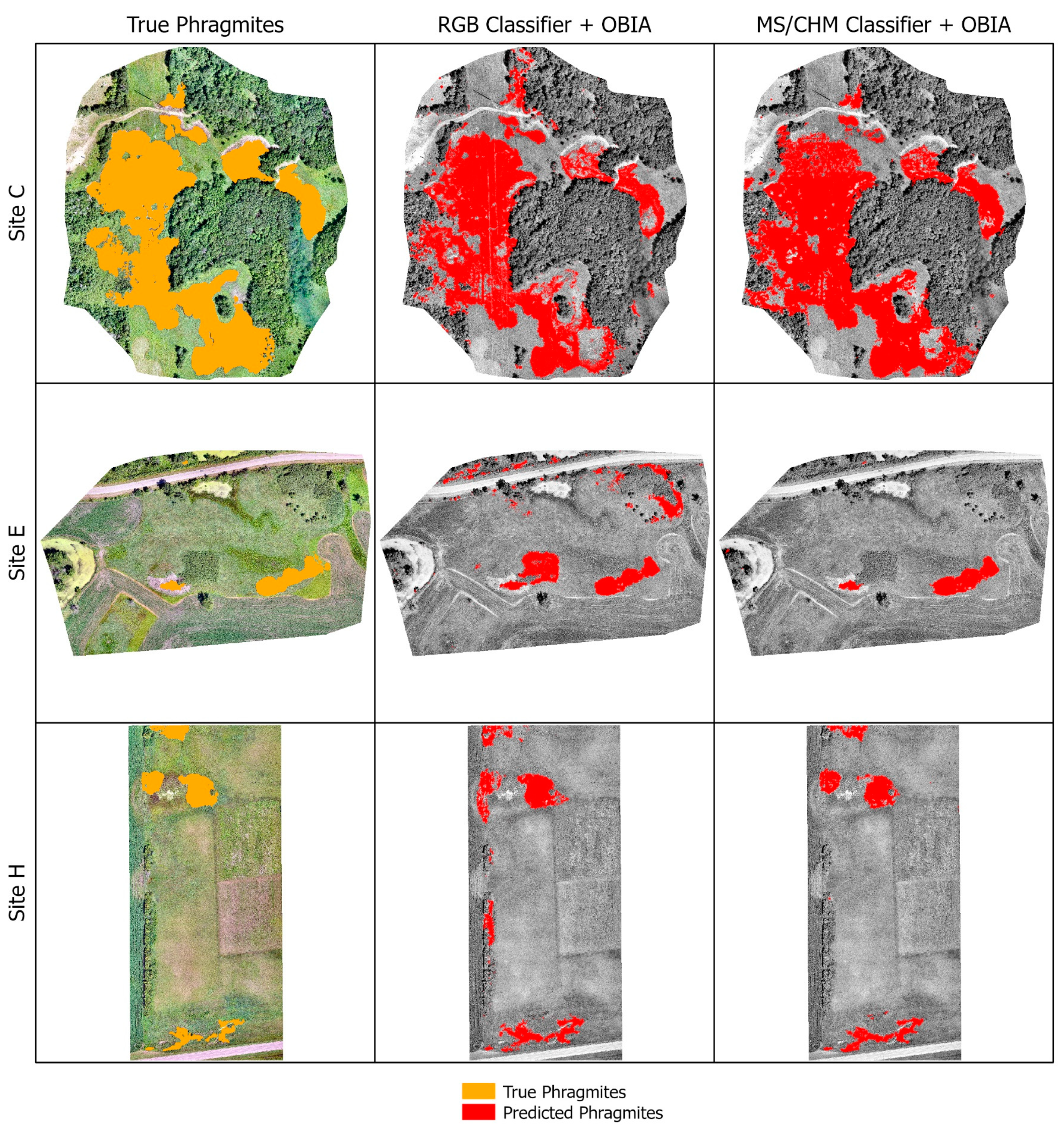
Figure 10.
Classification of Phragmites (red) using the RGB classifier with the post-ML OBIA rule set and the MS/CHM classifier with the post-ML OBIA rule set at the three validation sites: Chisago City Property (Site C), Wabasha property (Site E), and the Swan Lake Wildlife Management Area (Site H). Everything not identified as Phragmites was classified as Not Phragmites. The true Phragmites location is provided as a reference (orange).
Table 1.
UAS collections at each study area. All RGB imagery (red, green, and blue spectral bands) was acquired at 121 m above ground level with 85% endlap and 70% sidelap. All multispectral (MS) imagery was acquired at 121 m above ground level with 75% endlap and sidelap.
Table 1.
UAS collections at each study area. All RGB imagery (red, green, and blue spectral bands) was acquired at 121 m above ground level with 85% endlap and 70% sidelap. All multispectral (MS) imagery was acquired at 121 m above ground level with 75% endlap and sidelap.
| Study Area | Collection Date | Hectares | RGB Resolution | MS Resolution | Weather |
|---|
| Delano WWTF | 15 July 2022 | 10.8 | 1.68 cm | 8.7 cm | Partly cloudy and light wind |
| Delano City Park | 15 July 2022 | 11.0 | 1.7 cm | 8.8 cm | Partly cloudy and light wind |
| Chisago City | 21 July 2022 | 23.4 | 1.66 cm | 8.4 cm | Partly cloudy and moderate wind |
| Wabasha | 12 August 2021 | 11.6 | 1.66 cm | 8.6 cm | Clear skies and moderate wind |
| Wabasha | 4 August 2022 | 11.3 | 1.5 cm | 7.5 cm | Clear skies and light wind |
| Chatfield WWTF | 3 August 2021 | 8.6 | 1.61 cm | 8.4 cm | Clear skies with light haze from wildfire smoke |
| Chatfield WWTF | 2 August 2022 | 13.2 | 1.5 cm | 7.3 cm | Clear skies and moderate wind |
| Swan Lake WMA | 19 July 2021 | 15.5 | 1.68 cm | 8.8 cm | Mostly clear and light wind |
Table 2.
Lidar collection periods for each study area.
Table 2.
Lidar collection periods for each study area.
| Study Area | County | Collection Period |
|---|
| Delano WWTF | Wright | 23 April–28 May 2008 |
| Delano City Park | Wright | 23 April–28 May 2008 |
| Chisago City | Chisago | 18–28 April 2007 |
| Wabasha | Wabasha | 18–24 November 2008 |
| Chatfield WWTF | Olmsted | 18–24 November 2008 |
| Swan Lake WMA | Nicollet | 8 April–5 May; 2–19 November 2010 |
Table 3.
Number of training image objects per cover class for the multispectral classification (MS) and RGB (red, green, and blue spectral bands) classification. Training samples were created using the multi-resolution segmentation in the Trimble eCognition Developer software. The RGB and MS training samples cover the same spatial extent, but the number of training samples per cover class varies due to different multi-resolution segmentation parameters.
| | Cover Class |
|---|
| Classification Type | Mowed Grass | Phragmites | Tree | Short Tree | Wetland | Agriculture |
|---|
| RGB | 9597 | 93,744 | 49,061 | 24,044 | 258,554 | 130,773 |
| MS | 68,546 | 294,178 | 111,684 | 58,093 | 809,093 | 198,417 |
Table 4.
Parameters included for the classification using the RGB UAS imagery (RGB classifier), the multispectral classification without a canopy height model (MS classifier), and the multispectral classification with a canopy height model derived from the RGB UAS imagery (MS/CHM classifier).
Table 4.
Parameters included for the classification using the RGB UAS imagery (RGB classifier), the multispectral classification without a canopy height model (MS classifier), and the multispectral classification with a canopy height model derived from the RGB UAS imagery (MS/CHM classifier).
| | RGB Classifier | MS Classifier | MS/CHM Classifier |
|---|
| Parameter |
|---|
| Brightness | X | X | X |
| Edge Contrast of Blue Band (Window: 10) | X | X | X |
| Edge Contrast of Green Band (Window: 10) | X | X | X |
| Edge Contrast of NDVI (Window: 10) | | X | X |
| Edge Contrast of NIR Band (Window: 10) | | X | X |
| Edge Contrast of CHM (Window: 10) | X | | X |
| Edge Contrast of Red Band (Window: 10) | X | X | X |
| Edge Contrast of Red Edge Band (Window: 10) | | X | X |
| Grey-Level Co-occurrence Matrix: Contrast | X | X | X |
| Grey-Level Co-occurrence Matrix: Homogeneity | X | X | X |
| Maximum Difference | X | X | X |
| Mean of Blue Band | X | X | X |
| Mean of Green Band | X | X | X |
| Mean of Green-Blue Ratio | X | X | X |
| Mean of NDRE | | X | X |
| Mean of CHM | X | | X |
| Mean of NDVI | | X | X |
| Mean of NIR Band | | X | X |
| Mean of Red Band | X | X | X |
| Mean of Red-Blue Ratio | X | X | X |
| Mean of Red Edge Band | | X | X |
| Mean of VARI | X | X | X |
| Mean of VDVI | X | | |
| Short Bitmask | X | | X |
| Standard Deviation of Blue Band | X | X | X |
| Standard Deviation of Green Band | X | X | X |
| Standard Deviation of NDRE | | X | X |
| Standard Deviation of CHM | X | | X |
| Standard Deviation of NDVI | | X | X |
| Standard Deviation of NIR Band | | X | X |
| Standard Deviation of Red Band | X | X | X |
| Standard Deviation of Red-Blue Ratio | X | X | X |
| Standard Deviation of Red Edge Band | | X | X |
| Standard Deviation of VARI | X | X | X |
| Standard Deviation of VDVI | X | | |
| 25th Quantile of CHM | X | | X |
| 90th Quantile of CHM | X | | X |
| Tall Bitmask | X | | X |
Table 5.
Validation points per cover class for each validation collection. A total of 150 points were created for the Phragmites class, and 200 points were created for the Not Phragmites class. The number of verified points and the number randomly selected from the verified points are provided.
Table 5.
Validation points per cover class for each validation collection. A total of 150 points were created for the Phragmites class, and 200 points were created for the Not Phragmites class. The number of verified points and the number randomly selected from the verified points are provided.
| Phragmites Class | Generated | Verified | Selected |
| Chisago City Property | 150 | 98 | 75 |
| Swan Lake WMA | 150 | 88 | 75 |
| Wabasha Property (2022) | 150 | 88 | 75 |
| Chatfield WWTF (2021) | 150 | 43 | 35 |
| Delano City Park | 150 | 43 | 35 |
| Not Phragmites Class | Generated | Verified | Selected |
| Chisago City Property | 200 | 151 | 100 |
| Swan Lake WMA | 200 | 191 | 100 |
| Wabasha Property (2022) | 200 | 196 | 100 |
| Chatfield WWTF (2021) | 200 | 194 | 70 |
| Delano City Park | 200 | 199 | 70 |
Table 6.
Validation assessment points for each of the three validation sites for the multispectral ensemble classification without a canopy height model and a post-ML OBIA rule set.
Table 6.
Validation assessment points for each of the three validation sites for the multispectral ensemble classification without a canopy height model and a post-ML OBIA rule set.
| | Phragmites Class | Not Phragmites Class |
|---|
| Site | Correct | Incorrect | Correct | Incorrect |
|---|
| Chisago City Property | 6 | 69 | 92 | 8 |
| Swan Lake WMA | 0 | 75 | 100 | 0 |
| Wabasha Property | 0 | 75 | 94 | 6 |
| Combined | 6 | 219 | 286 | 14 |
Table 7.
User’s Accuracy (UA), Producer’s Accuracy (PA), Overall Accuracy (OA), and Matthews Correlation Coefficient (MCC) values for the multispectral ensemble classification without a canopy height model and a post-ML OBIA rule set.
Table 7.
User’s Accuracy (UA), Producer’s Accuracy (PA), Overall Accuracy (OA), and Matthews Correlation Coefficient (MCC) values for the multispectral ensemble classification without a canopy height model and a post-ML OBIA rule set.
| | Phragmites Class | Not Phragmites Class | | |
|---|
| Site | UA (%) | PA (%) | UA (%) | PA (%) | OA (%) | MCC |
|---|
| Chisago City Property | 43 | 8 | 57 | 92 | 56 | 0 |
| Swan Lake WMA | N/A | 0 | 57 | 100 | 57 | 0 |
| Wabasha Property | 0 | 0 | 56 | 94 | 54 | −0.16 |
| Combined | 30 | 3 | 57 | 95 | 56 | −0.05 |
Table 8.
Validation assessment points for the multispectral ensemble classification with a canopy height model but without a post-ML OBIA rule set.
Table 8.
Validation assessment points for the multispectral ensemble classification with a canopy height model but without a post-ML OBIA rule set.
| Site | Phragmites Class | Not Phragmites Class |
|---|
| Correct | Incorrect | Correct | Incorrect |
|---|
| Chisago City Property | 43 | 32 | 98 | 2 |
| Swan Lake WMA | 47 | 28 | 99 | 1 |
| Wabasha Property | 41 | 34 | 98 | 2 |
| Combined | 131 | 94 | 295 | 5 |
Table 9.
User’s Accuracy (UA), Producer’s Accuracy (PA), Overall Accuracy (OA), and Matthews Correlation Coefficient (MCC) values for the multispectral ensemble classification with a canopy height model but without a post-ML OBIA rule set.
Table 9.
User’s Accuracy (UA), Producer’s Accuracy (PA), Overall Accuracy (OA), and Matthews Correlation Coefficient (MCC) values for the multispectral ensemble classification with a canopy height model but without a post-ML OBIA rule set.
| | Phragmites Class | Not Phragmites Class | | |
|---|
| Site | UA (%) | PA (%) | UA (%) | PA (%) | OA (%) | MCC |
|---|
| Chisago City Property | 96 | 57 | 75 | 98 | 81 | 0.63 |
| Swan Lake WMA | 98 | 57 | 75 | 98 | 83 | 0.68 |
| Wabasha Property | 95 | 55 | 74 | 98 | 79 | 0.61 |
| Combined | 96 | 58 | 76 | 98 | 81 | 0.64 |
Table 10.
Validation assessment points for the multispectral ensemble classification with both a canopy height model and post-ML OBIA rule set.
Table 10.
Validation assessment points for the multispectral ensemble classification with both a canopy height model and post-ML OBIA rule set.
| | Phragmites Class | Not Phragmites Class |
|---|
| Site | Correct | Incorrect | Correct | Incorrect |
|---|
| Chisago City Property | 66 | 9 | 90 | 10 |
| Swan Lake WMA | 52 | 23 | 100 | 0 |
| Wabasha Property | 69 | 6 | 100 | 0 |
| Combined | 187 | 38 | 290 | 10 |
Table 11.
User’s Accuracy (UA), Producer’s Accuracy (PA), Overall Accuracy (OA), and Matthews Correlation Coefficient (MCC) values for the multispectral ensemble classification with both a canopy height model and a post-ML OBIA rule set.
Table 11.
User’s Accuracy (UA), Producer’s Accuracy (PA), Overall Accuracy (OA), and Matthews Correlation Coefficient (MCC) values for the multispectral ensemble classification with both a canopy height model and a post-ML OBIA rule set.
| | Phragmites Class | Not Phragmites Class | | |
|---|
| Site | UA (%) | PA (%) | UA (%) | PA (%) | OA (%) | MCC |
|---|
| Chisago City Property | 87 | 88 | 91 | 90 | 89 | 0.78 |
| Swan Lake WMA | 100 | 69 | 81 | 100 | 87 | 0.75 |
| Wabasha Property | 100 | 92 | 94 | 100 | 97 | 0.93 |
| Combined | 95 | 83 | 88 | 97 | 91 | 0.82 |
Table 12.
Validation assessment points for each of the three multispectral ensemble classifications at the two withheld validation sites: the 2021 Chatfield WWTF collection and the Delano City Park.
Table 12.
Validation assessment points for each of the three multispectral ensemble classifications at the two withheld validation sites: the 2021 Chatfield WWTF collection and the Delano City Park.
| | Phragmites Class | Not PhragmitesClass |
| Delano City Park | Correct | Incorrect | Correct | Incorrect |
| MS | 5 | 30 | 60 | 10 |
| MS/CHM | 15 | 20 | 64 | 6 |
| MS/CHM + OBIA | 1 | 34 | 70 | 0 |
| Chatfield WWTF (2021) | Correct | Incorrect | Correct | Incorrect |
| MS | 27 | 8 | 64 | 6 |
| MS/CHM | 31 | 4 | 68 | 2 |
| MS/CHM + OBIA | 27 | 8 | 70 | 0 |
Table 13.
User’s Accuracy (UA), Producer’s Accuracy (PA), Overall Accuracy (OA), and Matthews Correlation Coefficient (MCC) values for the three multispectral ensemble classification at the two withheld validation sites: the 2021 Chatfield WWTF collection and the Delano City Park.
Table 13.
User’s Accuracy (UA), Producer’s Accuracy (PA), Overall Accuracy (OA), and Matthews Correlation Coefficient (MCC) values for the three multispectral ensemble classification at the two withheld validation sites: the 2021 Chatfield WWTF collection and the Delano City Park.
| | PhragmitesClass | NotPhragmites Class | | |
| Delano City Park | UA (%) | PA (%) | UA (%) | PA (%) | OA (%) | MCC |
| MS | 50 | 14 | 67 | 86 | 62 | 0 |
| MS/CHM | 71 | 43 | 76 | 91 | 75 | 0.4 |
| MS/CHM + OBIA | 100 | 3 | 67 | 100 | 68 | 0.14 |
| Chatfield WWTF (2021) | UA (%) | PA (%) | UA (%) | PA (%) | OA (%) | MCC |
| MS | 82 | 77 | 89 | 91 | 87 | 0.7 |
| MS/CHM | 94 | 89 | 94 | 89 | 94 | 0.87 |
| MS/CHM + OBIA | 100 | 77 | 90 | 100 | 92 | 0.83 |
Table 14.
Validation assessment points for the RGB ensemble classification without the post-ML OBIA rule set.
Table 14.
Validation assessment points for the RGB ensemble classification without the post-ML OBIA rule set.
| | Phragmites Class | Not Phragmites Class |
|---|
| Site | Correct | Incorrect | Correct | Incorrect |
|---|
| Chisago City Property | 58 | 17 | 92 | 8 |
| Swan Lake WMA | 40 | 35 | 94 | 6 |
| Wabasha Property | 68 | 7 | 97 | 3 |
| Combined | 166 | 59 | 283 | 17 |
Table 15.
User’s Accuracy (UA), Producer’s Accuracy (PA), Overall Accuracy (OA), and Matthews Correlation Coefficient (MCC) values for the RGB ensemble classification without a post-ML OBIA rule set.
Table 15.
User’s Accuracy (UA), Producer’s Accuracy (PA), Overall Accuracy (OA), and Matthews Correlation Coefficient (MCC) values for the RGB ensemble classification without a post-ML OBIA rule set.
| | Phragmites Class | Not Phragmites Class | | |
|---|
| Site | UA (%) | PA (%) | UA (%) | PA (%) | OA (%) | MCC |
|---|
| Chisago City Property | 88 | 77 | 84 | 92 | 86 | 0.71 |
| Swan Lake WMA | 87 | 53 | 73 | 94 | 77 | 0.56 |
| Wabasha Property | 96 | 91 | 93 | 97 | 94 | 0.88 |
| Combined | 91 | 80 | 86 | 94 | 86 | 0.74 |
Table 16.
Validation assessment points for the RGB ensemble classification with the post-ML OBIA rule set.
Table 16.
Validation assessment points for the RGB ensemble classification with the post-ML OBIA rule set.
| | Phragmites Class | Not Phragmites Class |
|---|
| Site | Correct | Incorrect | Correct | Incorrect |
|---|
| Chisago City Property | 60 | 15 | 93 | 7 |
| Swan Lake WMA | 49 | 26 | 97 | 3 |
| Wabasha Property | 68 | 7 | 97 | 3 |
| Combined | 177 | 48 | 287 | 13 |
Table 17.
User’s Accuracy (UA), Producer’s Accuracy (PA), Overall Accuracy (OA), and Matthews Correlation Coefficient (MCC) values for the RGB ensemble classification with the post-ML OBIA rule set.
Table 17.
User’s Accuracy (UA), Producer’s Accuracy (PA), Overall Accuracy (OA), and Matthews Correlation Coefficient (MCC) values for the RGB ensemble classification with the post-ML OBIA rule set.
| | Phragmites Class | Not Phragmites Class | | |
|---|
| Site | UA (%) | PA (%) | UA (%) | PA (%) | OA (%) | MCC |
|---|
| Chisago City Property | 90 | 80 | 86 | 93 | 87 | 0.74 |
| Swan Lake WMA | 94 | 65 | 79 | 97 | 83 | 0.67 |
| Wabasha Property | 96 | 91 | 93 | 97 | 94 | 0.88 |
| Combined | 93 | 79 | 86 | 96 | 88 | 0.76 |
Table 18.
Validation assessment points for the RGB classifier both with and without the post-ML OBIA rule set at the two withheld validation sites: the 2021 Chatfield WWTF collection and the Delano City Park.
Table 18.
Validation assessment points for the RGB classifier both with and without the post-ML OBIA rule set at the two withheld validation sites: the 2021 Chatfield WWTF collection and the Delano City Park.
| | Phragmites Class | Not Phragmites Class |
| Delano City Park | Correct | Incorrect | Correct | Incorrect |
| RGB Classifier | 28 | 7 | 55 | 15 |
| RGB Classifier + OBIA | 24 | 11 | 69 | 1 |
| Chatfield WWTF (2021) | Correct | Incorrect | Correct | Incorrect |
| RGB Classifier | 34 | 1 | 68 | 2 |
| RGB Classifier + OBIA | 34 | 1 | 68 | 2 |
Table 19.
User’s Accuracy (UA), Producer’s Accuracy (PA), Overall Accuracy (OA), and Matthews Correlation Coefficient (MCC) values for the RGB classifier both with and without the post-ML OBIA rule set at the two withheld validation sites: the 2021 Chatfield WWTF collection and the Delano City Park.
| | Phragmites Class | Not Phragmites Class | | |
| Delano City Park | UA (%) | PA (%) | UA (%) | PA (%) | OA (%) | MCC |
| RGB Classifier | 65 | 80 | 89 | 79 | 79 | 0.56 |
| RGB Classifier + OBIA | 96 | 69 | 86 | 99 | 89 | 0.74 |
| Chatfield WWTF (2021) | UA (%) | PA (%) | UA (%) | PA (%) | OA (%) | MCC |
| RGB Classifier | 94 | 97 | 99 | 97 | 97 | 0.94 |
| RGB Classifier + OBIA | 94 | 97 | 99 | 97 | 97 | 0.94 |


