Inversion of Leaf Area Index in Citrus Trees Based on Multi-Modal Data Fusion from UAV Platform

Abstract

The leaf area index (LAI) is an important growth indicator used to assess the health status and growth of citrus trees. Although LAI estimation based on unmanned aerial vehicle (UAV) platforms has been widely used for field crops, mainly focusing on food crops, less research has been reported on the application to fruit trees, especially citrus trees. In addition, most studies have used single-modal data for modeling, but some studies have shown that multi-modal data can be effective in improving experimental results. This study utilizes data collected from a UAV platform, including RGB images and point cloud data, to construct single-modal regression models named VoVNet (using RGB data) and PCNet (using point cloud data), as well as a multi-modal regression model called VPNet (using both RGB data and point cloud data). The LAI of citrus trees was estimated using deep neural networks, and the results of two experimental hyperparameters (loss function and learning rate) were compared under different parameters. The results of the study showed that VoVNet had Mean Squared Error (MSE), Mean Absolute Error (MAE), and R-Squared (R²) of 0.129, 0.028, and 0.647, respectively. In comparison, PCNet decreased by 0.051 and 0.014 to 0.078 and 0.014 for MAE and MSE, respectively, while R² increased by 0.168 to 0.815. VPNet decreased by 0% and 42.9% relative to PCNet in terms of MAE and MSE to 0.078 and 0.008, respectively, while R² increased by 5.6% to 0.861. In addition, the use of loss function L1 gave better results than L2, while a lower learning rate gave better results. It is concluded that the fusion of RGB data and point cloud data collected by the UAV platform for LAI estimation is capable of monitoring citrus trees’ growth process, which can help farmers to track the growth condition of citrus trees and improve the efficiency and quality of orchard management.

1. Introduction

Citrus trees are an important cash crop belonging to the genus Citrus (Rutaceae). It has a wide area of cultivation worldwide and is an economic pillar in many developing countries [1]. The healthy growth and development of citrus trees is an important guarantee of yield [2]. In order to ensure the high yield and quality of citrus trees, their growth needs to be monitored in a timely manner.

In the field of agriculture, UAVs equipped with various intelligent sensors and devices [3] can be utilized for multiple tasks, including pesticide spraying [4], harvesting [5], field planning [6], and crop growth monitoring [7,8,9]. Among them, the monitoring of crop growth is an important function of UAVs [10]. By using various sensors and cameras to acquire crop growth data, and subsequently processing and analyzing the data [11], information such as plant height [12], yield prediction [13], leaf area index [14], and carotenoid content [15] can be obtained. Particularly, the leaf area index is crucial for monitoring crop growth [16] as it enables the accurate diagnosis and management of crop growth conditions.

The leaf area index (LAI) is the sum of plant leaf area per unit of land area and is an important indicator of plant growth and ecosystems [17]. LAI is very important in ecological biophysics. By monitoring and analyzing LAI, it is possible to assess the growth rate, health status, and growth potential of crops and to take timely management measures, such as applying fertilizers, irrigation, and pest control, to maximize crop yield and quality [18]. Generally, the measurement of LAI is divided into direct and indirect methods [19]. The direct method is traditional and destructive, and although it gives the most accurate results, it is difficult to apply it to large-scale farmland measurements [20]. Indirect methods mainly use optical methods and inclined point sampling methods to obtain LAI [20]. The current widely used optical instruments are classified as radiation-based and image-based measurements. Representative instruments of the former are LAI-2000 (Licor Inc., Lincoln, NE, USA), TRAC (Wave Engineering Co., Nepean, ON, Canada), Sunscan (Delta-T Inc., Cambridge, UK), etc. The advantage of radiation measurement instruments is that they are fast and easy to measure, but they are susceptible to weather and often need to work on sunny days and correct for aggregation effects [21]. Typical instruments for image-based measurements are CI-110 (CID Inc., Washington, DC, USA), Image Analysis System (Delta-T Inc., Cambridge, UK), WinScanopy (Regent Inc., Thunder Bay, ON, Canada), etc. Among them, CI-110 is suitable for a low plant canopy and has high measurement accuracy, which is popular for LAI measurements in agricultural fields [22,23,24].

For estimating the LAI of citrus trees, optical instruments are currently the common measurement tools, but they require labor-intensive and costly efforts to measure the LAI of each citrus tree. In contrast, the use of remote sensing to estimate the LAI of citrus trees can save significant time and labor costs, where multiple data sources are often utilized for estimation. For instance, vegetation feature parameters such as the leaf area and leaf distribution density can be extracted from RGB images to calculate the LAI [25,26]. Additionally, point cloud data can be utilized to estimate the leaf area index by measuring the height and density of the plant canopy [27]. Hyperspectral data, on the other hand, can infer the leaf area index by continuously acquiring spectral reflectance information of vegetation within a narrow wavelength range [28]. Furthermore, vegetation indices can be employed to estimate the leaf area index by analyzing the spectral reflectance of vegetation [29].

In terms of data type selection, the use of remotely sensed images taken by UAVs for estimation can reduce the time to obtain LAI and reduce the effects of topographic difficulties [30]. Hasan et al. [31] used parameters from UAV RGB images to estimate the LAI of winter wheat. Based on gray correlation analysis, five vegetation indices, such as Visible Atmospheric Resistance Index (VARI), were selected to develop models for estimating the LAI of winter wheat. The results showed that partial least squares regression (PLSR) models based on VARI, RGBVI, B, and GLA had the best prediction accuracy among all regression models (R² = 0.776, root mean square error (RMSE) = 0.468, and residual prediction deviation (RPD) = 1.838). Yamaguchi et al. [32] compared the LAI estimation model developed via deep learning (DL) using RGB images with three other practical methods: a plant canopy analyzer (PCA), regression models based on color indices (CIs) obtained from an RGB camera, and vegetation indices (VIs) obtained from a multispectral camera. The results showed that the estimation accuracy of the DL model built with RGB images (R² = 0.963, RMSE = 0.334) was higher than that of the PCA (R² = 0.934, RMSE = 0.555) and CIs-based regression models (R² = 0.802–0.947, RMSE = 0.401–1.13), and was comparable to that of the VIs-based regression models (R² = 0.917–0.976, RMSE = 0.332–0.644).

Point cloud data can provide very high measurement accuracy, which can avoid human error and measurement errors and improve the reliability and accuracy of data compared to traditional measurement methods [27,33,34]. Yang et al. [35] proposed a 3-D point cloud method using UAV to automatically calculate crop-effective LAI (LAIe). The method accurately estimated LAIe by projecting 3-D point cloud data of winter wheat onto the hemisphere and calculating the gap fraction using both single-angle inversion and multi-angle inversion methods. The results showed that the calculated LAIe had a good linear correlation with the LAIe measured via digital hemispheric photography in the field, and the stereographic projection multi-angle inversion method had the highest accuracy, with an R² of 0.63. Song et al. [36] used 3-D point cloud data based on UAVs to automatically calculate LAIe. The method used high-resolution RGB images to generate point cloud data and the 3-D spatial distribution of vegetation and bare ground points and calculate the gap fraction and LAIe from a UAV-based 3-D point cloud dataset. The results showed a strong correlation between the derived LAIe and ground-based digital hemispherical photography (R² = 0.76).

Although the estimation of LAI has been widely studied, it has been applied to fruit trees in large fields with relatively little and less than optimal results, and relatively little research has been conducted on citrus trees. Mazzini et al. [37] found that the leaf length, leaf width, and leaf length times leaf width were all strongly correlated with the leaf area and that a linear equation using leaf length times leaf width as a variable was the most accurate and reliable model. Dutra et al. [38] developed separate empirical equations for LAI for single and compound-leafed citrus trees. Raj et al. [39] used RGB images taken by UAV to estimate the LAI of a citrus canopy, and the R² of the estimated value with the LAI value measured by the ground instrument was 0.73.

In some studies, better estimation results can be obtained by fusing multi-modal data than using single-modal data. Maimaitijiang et al. [40] estimated soybean yields (R² = 0.72, RMSE = 0.159) using RGB and multispectral and thermal sensors within the framework of a deep neural network. Zhang et al. [41] used UAV spectral parameters with texture feature data to estimate the LAI of kiwifruit orchard via the stepwise regression method and random forest approach (R² = 0.947, RMSE = 0.048, nRMSE = 7.99%). Wu et al. [42] used UAV images and spectral, structural, and thermal characteristics of a wheat canopy to estimate the LAI of wheat using the random forest approach and support vector machine regression (R² = 0.679, RMSE = 1.231).

LAI estimation using deep neural networks is the main method for connecting different data sources, and the main advantage is its ability to learn complex, nonlinear mapping relationships. Compared to traditional linear models, deep neural networks have stronger capabilities in capturing the nonlinear mapping patterns between LAI and input data. By learning from large-scale training data, deep neural networks can accurately estimate LAI values. The multi-modal data fusion used in this study is a combination of RGB data and point cloud data, thus increasing the richness of the data. RGB data provide color and texture information, while point cloud data provide information on position, size, and orientation in 3-D space. This fusion enhances data robustness, reduces reliance on a single data source, and improves model stability and adaptability.

In this study, RGB data and point cloud data acquired by a UAV platform were used to construct regression models for single-modal data and multi-modal data to estimate the LAI of citrus trees using deep neural networks, and a comparative analysis was conducted to verify whether multi-modal data are more beneficial for estimating the LAI of citrus trees.

2. Materials and Methods

2.1. Study Area Overview

The study site is located in a citrus orchard plantation in Huangtian Town, Sihui City, Zhaoqing City, Guangdong Province, China (23°36′N, 112°68′E), as shown in Figure 1. The climatic conditions were subtropical monsoonal, with an average annual temperature of 21 °C and an annual precipitation of 1800 mm. The 110 citrus trees selected for this study were of similar age and growing in good environmental conditions in March of 2023. These citrus trees were at the stage of spring shoot growth. The management of this stage involves two aspects: promoting shoot growth and preventing pests and diseases, as well as managing the flowering of mature and young trees. Effective management at this stage is crucial for subsequent flowering and fruiting.

2.2. Data Acquisition

2.2.1. Measuring LAI of Citrus Trees

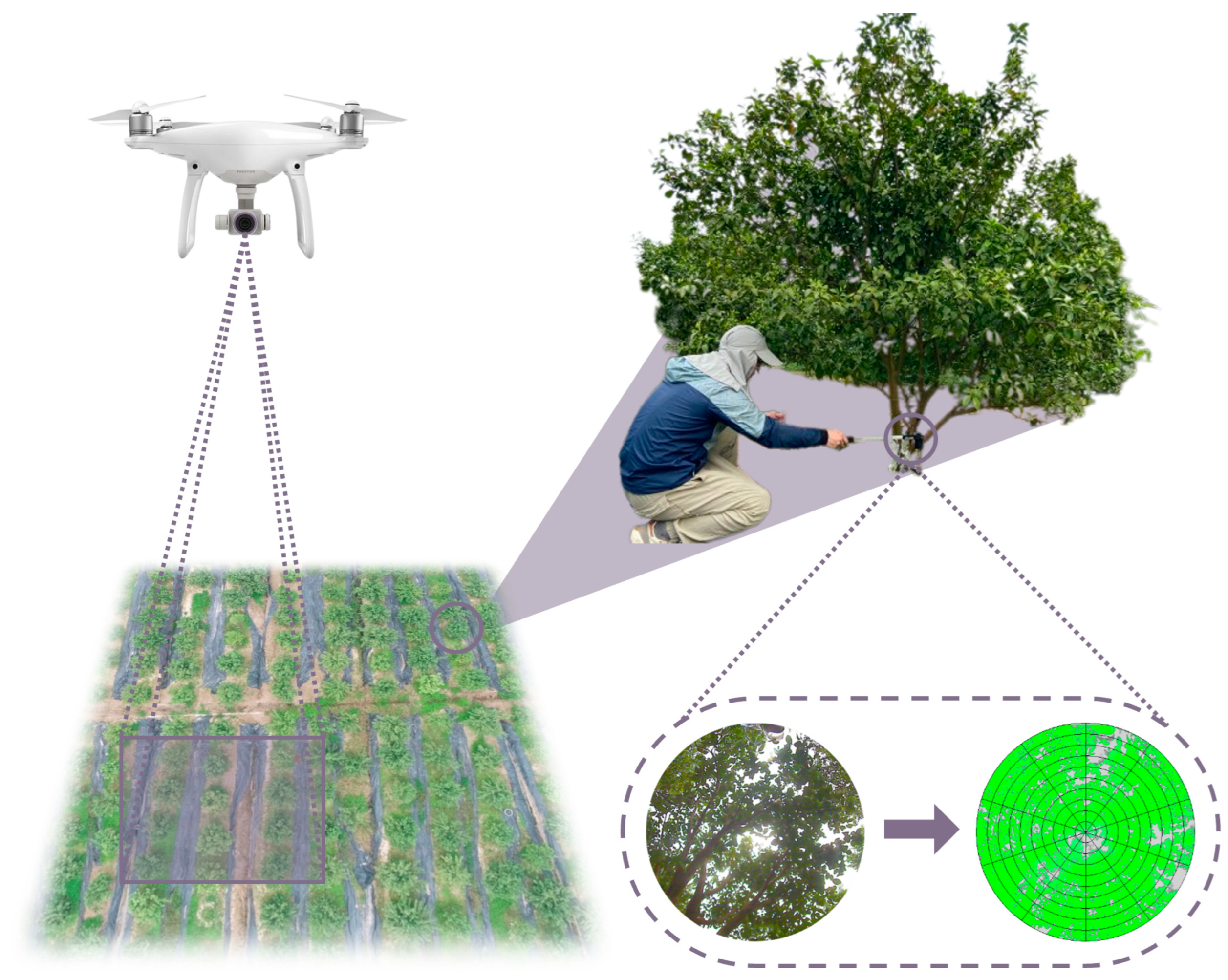
Two image-acquisition measurements were taken using Plant Canopy Imager CI-110 (CID Inc., Washington, DC, USA) on 110 citrus trees at approximately 20 cm from the ground and 20 cm from the trunk, and the average was taken as the LAI value of the citrus tree [22,43]. CI-110 is a non-destructive and efficient tool for measuring plant canopy characteristics with a self-leveling hemispherical lens, a built-in touchscreen display, a GPS and compass, and 24 PAR sensors. LAI was calculated using the CI-110 Plant Canopy Analysis software. During image acquisition, the brightness and contrast were adjusted so that all plant parts in the image appeared green to obtain an accurate processing section. The captured images were imported into this software for further processing by adjusting parameters such as brightness, contrast, and gamma to derive a more accurate LAI. The data collection was conducted on the mornings of 2–3 March 2023. The weather was overcast, which provided favorable lighting conditions for image acquisition and minimized the impact of intense sunlight [44].

2.2.2. UAV RGB Image Acquisition

The DJI Phantom 4 RTK (SZ DJI Technology Co., Shenzhen, China) was used for aerial oblique images to obtain high-quality RGB images for 3-D reconstruction and point cloud data generation of the citrus orchard. The UAV has a 1-inch, 20-megapixel CMOS sensor with a centimeter-level navigation and positioning system and a high-performance imaging system to accurately locate and photograph the area, thus ensuring image quality. The flight time was chosen at midday, with clear and stable weather and good lighting conditions. In this study, a GS RTK APP platform supporting route planning was used for setup to automate flight and route planning. This made the whole process more efficient, accurate, and safe. The specific flight parameters are shown in

Table 1. Flight parameter settings.

Parameter	Value/Method
Flight altitude	50 m
Flight speed	3 m/s
Shooting mode	Timed shooting
Pitch gimbal	−90, −60, −45
Side overlap rate	80%
Forward overlap rate	80%

. A total of 1072 images were captured, each with a size of 5472 × 3648 pixels. During the process, the UAV automatically recorded the latitude, longitude, and altitude at that time for subsequent 3-D reconstruction. The acquisition process is shown in Figure 2, which coincides with the LAI data collection time.

2.3. Data Pre-Processing

2.3.1. Acquisition of RGB Images of Citrus Trees

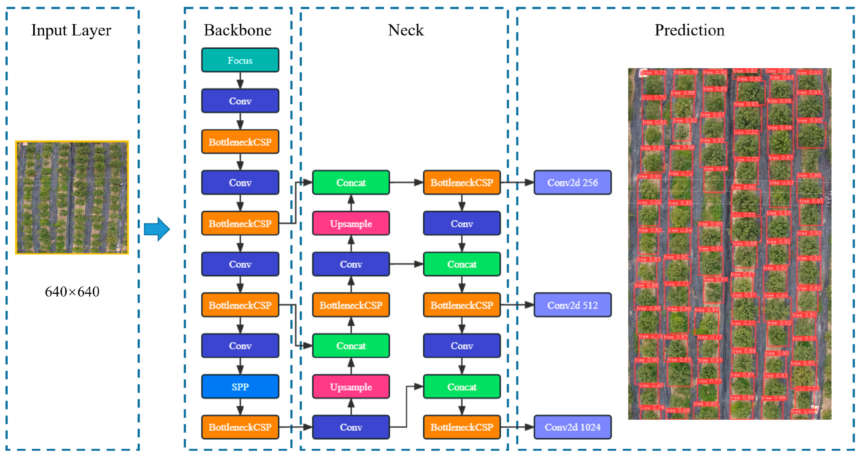
The You Only Look Once-v5s (YOLO-v5s) model [45] was used to accurately extract a single citrus tree from the UAV RGB image for target recognition. The model adopts a lightweight structure design and optimization, which can improve the detection speed while ensuring accuracy and achieving the requirement of real-time detection. The YOLO-v5s model has the advantages of high accuracy, high efficiency, and wide scalability and is an excellent target-detection algorithm with a weight size of 13.7 MB. The structural diagram is shown in Figure 3. A total of 635 images of citrus trees were used as the model training dataset, and the images were labeled with the labelImg software to label the location and category of citrus trees, with a total of 76,665 labeled boxes. The accuracy, recall, and map_0.5 of the model were 0.98, 0.98, and 0.99, respectively, which had good recognition accuracy. The recognized target citrus trees would be cropped and saved as RGB images with 3 channels of red, green, and blue, as shown in Figure 4.

2.3.2. Acquisition of Point Cloud Data of Citrus Tree

The first step was to reconstruct the 3-D model of the oblique images acquired by the UAV using Pix4Dmapper software (Pix4D Co., Prilly, Switzerland). Pix4Dmapper can convert UAV or other aerial image data into high-precision maps, models, and point cloud data and supports the input and output of multiple data formats. Import the oblique images into Pix4Dmapper, determine the datum as World Geodetic System 1984, the coordinate system as WGS 84, the camera model as FC6310R_8.8_5472×3648 (RGB), and select the “3D Models” processing option template. The 3-D reconstruction model of the citrus orchard was finally obtained after processing by the program. The point cloud data of the citrus orchard were imported into CloudCompare software, which provides powerful point cloud processing and analysis functions, including point cloud alignment, filtering, segmentation, reconstruction, analysis, and visualization operations. In the software, the citrus orchard was first cropped to remove point clouds outside the study area, which can be more convenient for manipulating the 3-D model. Next, the citrus trees were cropped to remove the ground point clouds to obtain the point cloud data of independent citrus trees. The specific process is shown in Figure 5. The citrus tree point cloud data were saved in txt file format, and each piece of point cloud data contained 6 parameter values, which were X-axis, Y-axis, Z-axis, red channel, green channel, and blue channel, as shown in

Table 2. Point cloud data display.

Point Cloud	X-Axis	Y-Axis	Z-Axis	Red	Green	Blue
1	655,215.95899963	2,592,974.80603027	6.21799994	113	138	92
2	655,215.96000671	2,592,974.75402832	6.15500021	146	178	123
3	655,215.96400452	2,592,974.74298096	6.14599991	149	178	123

.

2.3.3. RGB Data Model

When processing RGB image data, models need to effectively capture features of different scales because RGB images contain rich color and texture information. Additionally, models need to have fast training and inference capabilities and operate efficiently in situations with limited computing resources. Therefore, VoVNet [46] is a good choice. The VoVNet is a convolutional neural network based on One-Shot Aggregation (OSA) modules, which is mainly available in three different configurations, vovnet-27-slim, vovnet-39, and vovnet-57. vovnet-27-slim was chosen for this study. The VoVNet is a Stage 1 consisting of three 3 × 3 convolutional layers, followed by a max pooling layer and four OSA modules connected to form Stages 2–5, and finally, an adaptive average pooling layer and a fully connected layer to form Stage 6. The OSA module is a modified DenseNet [47]; it only aggregates all the previous layers at once at the end, which can reduce the memory access cost and improve the GPU computational efficiency, and it can capture the multiscale receptive domain and effectively present a diverse representation of features, which is good for handling multiscale objects. Its network diagram is shown in Figure 6.

2.3.4. Point Cloud Data Model

Point cloud data contain rich geometric and spatial information. To capture both local and global features of the point cloud, the model needs to incorporate one-dimensional convolutional layers for convolution operations on the data. However, due to the large quantity of point cloud data, not reducing or aggregating the data will result in a significant computational load and waste of computational resources. Therefore, PCNet was used as a model for point cloud data processing, as shown in Figure 7. The PCNet contains multiple convolutional layers, pooling layers, fully connected layers, and activation functions. Specifically, the first layer of the model is a 1-dimensional convolutional layer with 1 input channels, 10 output channels, a convolutional kernel size of 3, and a step size of 2, followed by a SELU activation function. The subsequent layers are similarly structured, where the number of input channels in each layer is the number of output channels in the previous layer. The last three layers of the model are fully connected layers, with 2048- and 1024-dimensional inputs and 1024- and 512-dimensional outputs for the first two layers, and each layer is followed by a ReLU activation function. The final fully connected layer has 512 and 1-dimensional inputs and outputs, respectively. It also includes an adaptive average pooling layer and a maximum pooling layer for extracting important information from the input features.

2.3.5. Multi-Modal Data Model

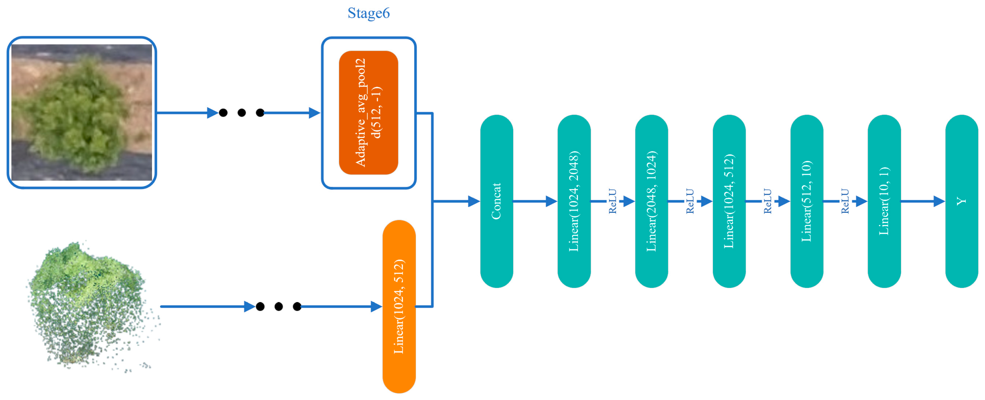
The network combining VoVNet and PCNet is VPNet, as shown in Figure 8. VoVNet removes the fully connected layer of Stage 6 from the original and keeps the adaptive level pooling layer, which is used for the adaptive connection between the convolutional layer and the fully connected layer to project high-dimensional features into the low-dimensional space. Stage 6 of VoVNet is connected to the penultimate fully connected layer of PCNet. The connection is followed by five fully connected layers, each of which has a ReLU activation function that enhances the nonlinear capability of the model. The input of the first fully connected layer is a vector of length 1024. The number of neurons in the fully connected layers is 2048, 1024, 512, and 10, and the last layer is 1 neuron for the output of the final prediction. The network is able to make full use of the features of different data, thus improving the prediction accuracy of the model.

2.4. Model Evaluation

In this study, three evaluation metrics, mean squared error (MSE), mean absolute error (MAE), and R-Squared (R²), were chosen to measure the predictive ability of the model.

MSE measures the predictive power of the model by calculating the squared difference between the predicted and true values. Its calculation formula is as follows:

$$\mathrm{MSE}=\frac{{\sum }_{\mathrm{i}=1}^{\mathrm{n}}{\left({\mathrm{y}}_{\mathrm{i}}-{\widehat{\mathrm{y}}}_{\mathrm{i}}\right)}^2}{\mathrm{n}}$$

(1)

MAE measures the predictive power of a model by calculating the absolute difference between the predicted and true values. It is calculated by the following formula:

$$\mathrm{MAE}=\frac{{\sum }_{\mathrm{i}=1}^{\mathrm{n}}\left|{\mathrm{y}}_{\mathrm{i}}-{\widehat{\mathrm{y}}}_{\mathrm{i}}\right|}{\mathrm{n}}$$

(2)

R² calculates the proportion of variance between the predicted and true values to measure the predictive power of the model. It is calculated by the following formula:

$${\mathrm{R}}^2=1-\frac{{\sum }_{\mathrm{i}=1}^{\mathrm{n}}{\left({\mathrm{y}}_{\mathrm{i}}-{\widehat{\mathrm{y}}}_{\mathrm{i}}\right)}^2}{{\sum }_{\mathrm{i}=1}^{\mathrm{n}}{\left({\mathrm{y}}_{\mathrm{i}}-{\stackrel{\mathrm{-}}{\mathrm{y}}}_{\mathrm{i}}\right)}^2}$$

(3)

where n denotes the number of samples and ${\mathrm{y}}_{\mathrm{i}}$ denotes the true value, ${\widehat{\mathrm{y}}}_{\mathrm{i}}$ denotes the predicted value, and ${\stackrel{-}{\mathrm{y}}}_{\mathrm{i}}$ denotes the average of the true values. Smaller MSE and MAE indicate better predictive ability of the model. Compared with MSE, MAE is more concerned with the absolute difference between the predicted and true values and has less influence on the outliers. R² has a range from 0 to 1, and the closer the value is to 1, the better the model’s prediction ability is.

3. Results

Different training hyperparameters can lead to different training results. Therefore, researchers typically refer to the experimental parameters used by others and combine them with their own experience to select appropriate model hyperparameters. In the preliminary experiments, different values and methods of hyperparameters were tried, and it was found that the loss function and learning rate were two hyperparameters that had a significant impact on the results. For the comparison experiments of these two hyperparameters, the full-scale experiment method was used, and the hyperparameters of the model were set as shown in

Table 3. Hyperparameter settings.

Parameter	Value/Method
Epochs	500
Batch Size	16
Optimizer	Adam
Loss Function	L1
	L2
Learning Rate	0.001
	0.0001
	0.00001

, with six sets of experiments. There were 110 groups of data in the dataset, and the ratio of the number of training, validation, and test set was 7:2:1.

3.1. Single-Modal Data for LAI Estimation of Citrus Trees

3.1.1. RGB Data for LAI Estimation of Citrus Trees

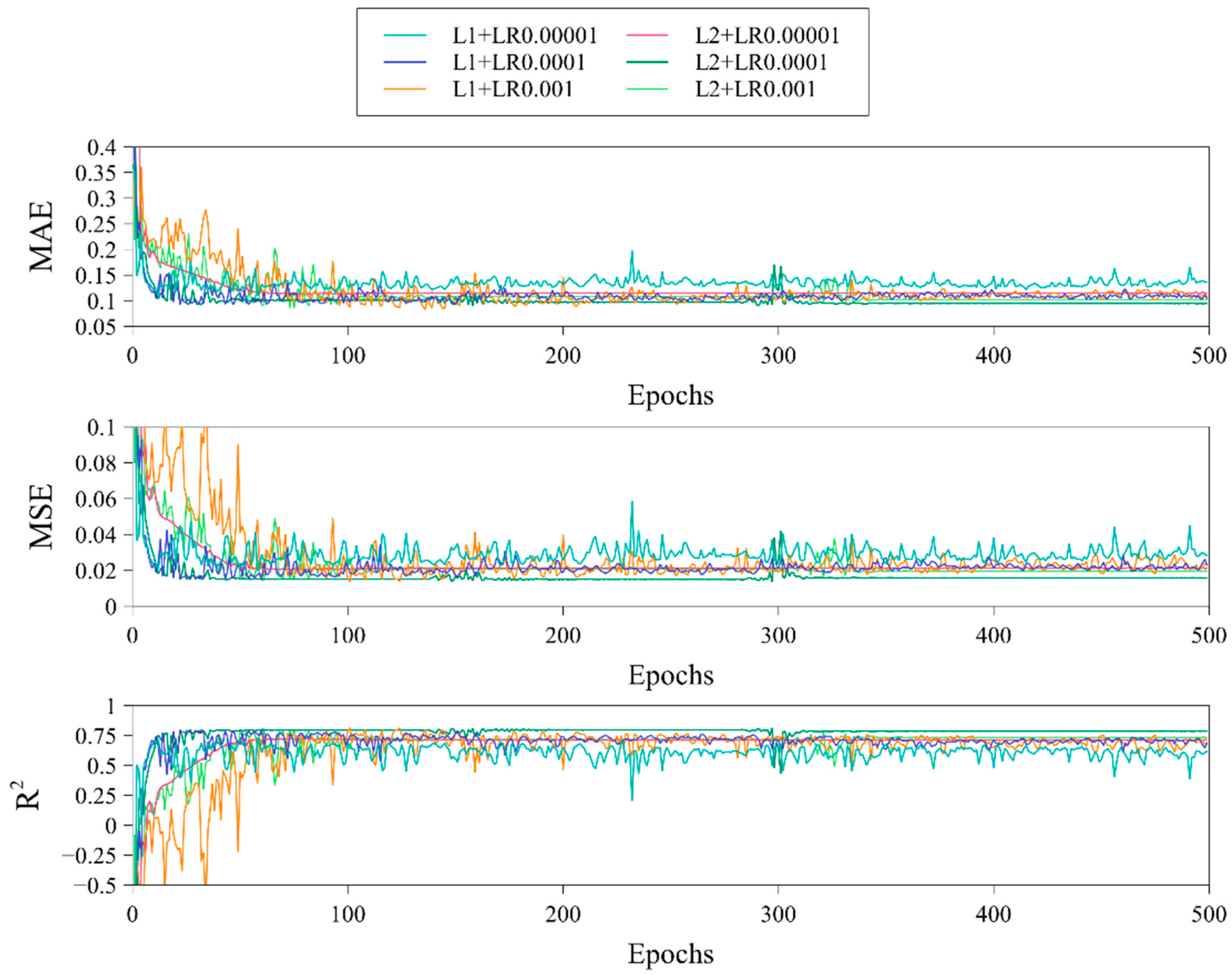
The training process of VoVNet using RGB data as training data is shown in Figure 9, and the results of the validation and test sets are shown in

Table 4. Training results of VoVNet with RGB images as training data.

Experimental Parameters	Validation			Test
	MAE	MSE	R2	MAE	MSE	R2
L1 + LR0.001	0.087	0.013	0.814	0.149	0.037	0.535
L1 + LR0.0001	0.092	0.015	0.795	0.15	0.034	0.575
L1 + LR0.00001	0.11	0.019	0.731	0.129	0.028	0.647
L2 + LR0.001	0.09	0.014	0.802	0.174	0.047	0.407
L2 + LR0.0001	0.092	0.013	0.813	0.149	0.035	0.561
L2 + LR0.00001	0.112	0.02	0.727	0.159	0.04	0.494

. Experimental parameter L1 + LR0.001 had larger data fluctuations during the training process than the other experimental parameters but had the best performance, possibly due to the larger learning rate setting, which caused the training data to constantly change during the search for the optimal solution, resulting in a strong fitting ability. The convergence speed of each experimental parameter group was relatively fast and had already converged before epoch 100. Experimental parameter L2 + LR0.00001 had the smallest data fluctuations during the training process and remained in a stable state, possibly due to the smaller learning rate setting, which found the local optimal solution and maintained a stable state.

The experimental results indicated that there was a significant difference between the evaluation metrics of the validation set and the test set. The MAE and MSE metrics of the validation set were between 0.087–0.112 and 0.013–0.02, respectively, and the R² metrics were between 0.727–0.814. However, the MAE and MSE metrics of the test set were between 0.129–0.174 and 0.028–0.047, respectively, and the R² metrics were between 0.407–0.647. Among them, the experimental parameters L1 + LR0.001 and L1 + LR0.00001 performed the best in the validation set and the test set, respectively. It was worth noting that the evaluation indicators on the test set were relatively lower than those on the validation set. This was because the test set was used to evaluate the generalization ability of the model, and the model may have overfit the training data during the training process, resulting in poor performance on the test set.

3.1.2. Point Cloud Data for LAI Estimation of Citrus Trees

The training process of PCNet using point cloud data as training data is shown in Figure 10, and the results of the validation and test sets are shown in

Table 5. PCNet training results with point cloud data as training data.

Experimental Parameters	Validation			Test
	MAE	MSE	R2	MAE	MSE	R2
L1 + LR0.001	0.079	0.01	0.864	0.123	0.021	0.74
L1 + LR0.0001	0.096	0.014	0.797	0.11	0.017	0.783
L1 + LR0.00001	0.085	0.01	0.863	0.078	0.014	0.815
L2 + LR0.001	0.133	0.026	0.644	0.194	0.058	0.279
L2 + LR0.0001	0.082	0.01	0.86	0.096	0.016	0.796
L2 + LR0.00001	0.093	0.015	0.791	0.126	0.026	0.671

. In the figure, it can be seen that the smaller the learning rate was, the slower the training convergence speed. Experimental parameter L1 + LR0.001 began to converge at about 50 epochs, while experimental parameter L1 + LR0.00001 began to converge at about 200 epochs. Experimental parameter L2 + LR0.001 showed significant data fluctuations during training, which may have been due to the large learning rate setting, hovering near the optimal value and accidentally causing gradient explosion.

In summary, the performance of experimental parameter L1 + LR0.00001 was the best. From the experimental data, the evaluation metrics of the test set were relatively lower than those of the validation set, indicating the possibility of overfitting, with the most obvious being experimental parameter L2 + LR0.001, which had MAE, MSE, and R² differences of −0.061, −0.032, and 0.365 between the validation and test sets, respectively. Compared with the results of point cloud data and RGB data, the test set of RGB data had more severe overfitting. In the test set, the MAE and MSE values of point cloud data were 0.051 and 0.014 lower than those of RGB data, respectively, and the R² value was 0.168 higher than that of RGB data. Overall, the results of point cloud data were better than those of RGB data, which may have been due to the fact that point cloud data are three-dimensional, while RGB data are two-dimensional, providing more information and resulting in better results.

3.2. Multi-Modal Data for LAI Estimation of Citrus Trees

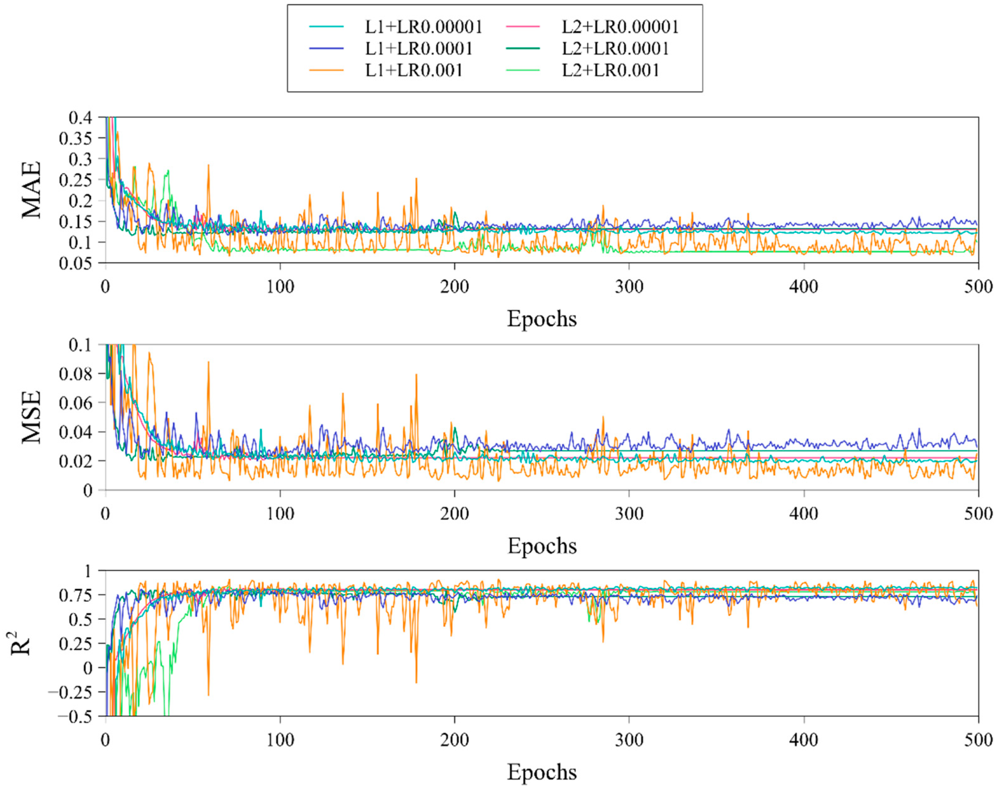
The training process of VPNet using RGB and point cloud data as training data is shown in Figure 11, and the results of the validation and test sets are presented in

Table 6. Training results of VPNet with multi-modal data as training data.

Experimental Parameters	Validation			Test
	MAE	MSE	R2	MAE	MSE	R2
L1 + LR0.001	0.062	0.005	0.914	0.078	0.008	0.861
L1 + LR0.0001	0.114	0.019	0.825	0.08	0.009	0.829
L1 + LR0.00001	0.117	0.017	0.841	0.066	0.010	0.805
L2 + LR0.001	0.076	0.009	0.834	0.079	0.009	0.849
L2 + LR0.0001	0.115	0.019	0.804	0.101	0.017	0.813
L2 + LR0.00001	0.124	0.02	0.816	0.081	0.012	0.765

. The training models of all experimental parameters converged quickly, with most of them having already converged by epoch 50. The amplitude of data fluctuations was generally small, with the most stable being the experimental parameter L2 + LR0.00001, which converged to a straight line after convergence, while the most volatile was the experimental parameter L1 + LR0.001, although it was the most effective. The training data of each experimental parameter were relatively close, and the results were better.

The MAE values in the test set data were generally below 0.1, the majority of the MSE values were below 0.01, and the majority of the R² values were above 0.8. The evaluation metrics were better than those of RGB and point cloud data, which may have been due to the fusion of data supplementing some information and achieving optimal training results. The performance of the experimental parameter L1 + LR0.001 was the best, possibly because the larger learning rate parameter setting made it easier for the model to avoid the limitations of locally optimal solutions and find better results, but the problem it brought was that the volatility of the training data was higher, and the stability was poorer.

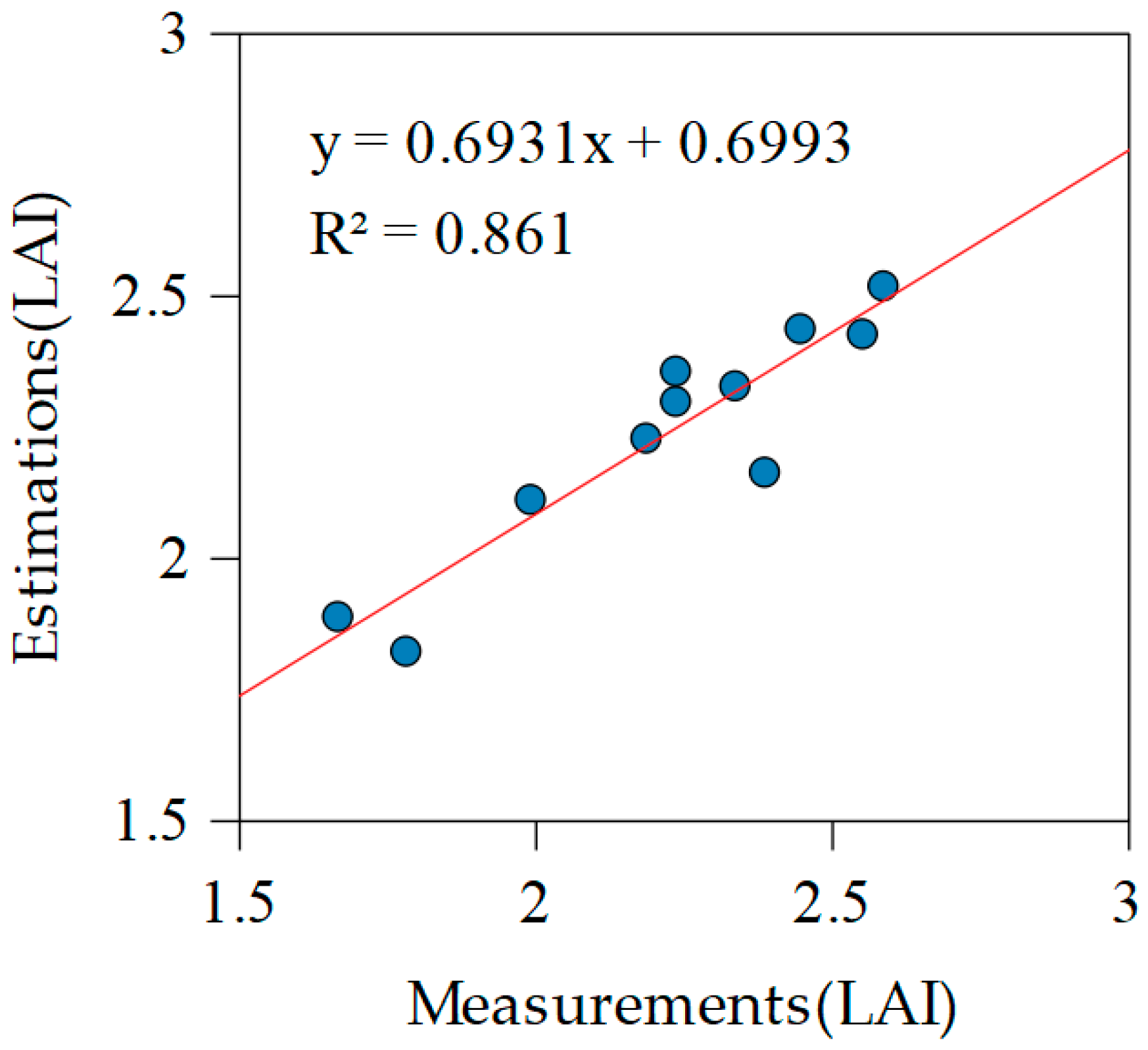
The multi-modal data were tested under the experimental parameter L1 + LR0.001, and the results are shown in Figure 12. By observing the graphs, it is clear that the fit of the multi-modal data is good.

3.3. Exploding and Vanishing Gradients of Multi-Modal Data Problem

In the experiments, it was found that the point cloud data have special properties, which may lead to the exploding gradients problem. The point cloud data consist of a large number of discrete points, each with 3-D coordinates and color information, for a total of six parameters. However, the values of these parameters vary greatly from one another, and this instability may be exacerbated when transformed into a 3-D tensor in a deep-learning model, leading to the emergence of the exploding gradients problem. Specifically, as the number of layers of the neural network increases, each layer of the activation function generates a certain amount of gradients. If these gradient values are large, the gradients accumulate during the backpropagation process, which may eventually cause the gradient values to become very large, even beyond the representation range of the computer, leading to the exploding gradients problem. This problem usually leads to models that do not converge or produce unstable results. To solve this problem, the data can be normalized to limit the values to the range of 0 to 1 to avoid the problems of neuron saturation and non-uniformity of the underlying metric units, thus avoiding the exploding gradients and speeding up the convergence of the neural network. The principle of normalization processing is shown in Formula (4). Examples of the normalization process are shown in

Table 7. Example of normalized point cloud data processing.

Method	Point Cloud	X-Axis	Y-Axis	Z-Axis	Red	Green	Blue
Original Data	1	655,215.95899963	2,592,974.80603027	6.21799994	113	138	92
	2	655,215.96000671	2,592,974.75402832	6.15500021	146	178	123
	3	655,215.96400452	2,592,974.74298096	6.14599991	149	178	123
Min-Max Normalization	1	0.010779881646158174	0.8936204728670418	0.049631731939932866	0.2924528301886793	0.3368983957219251	0.2431192660550459
	2	0.00040218885987997055	0.8812293692026287	0.018224273530279778	0.48584905660377353	0.588235294117647	0.408256880733945
	3	0.0019987597479484975	0.8763324494939297	0.014734433142619796	0.5	0.588235294117647	0.408256880733945

.

$$\mathrm{f}\left(\mathrm{x}\right)=\frac{\mathrm{x}-\min \left(\mathrm{x}\right)}{\max \left(\mathrm{x}\right)-\min \left(\mathrm{x}\right)}$$

(4)

In PCNet, the problem of vanishing gradients could occur when using the ReLU activation function after the convolution and pooling layers. This was due to the fact that the weights may have negative values during backpropagation, which would become 0 after ReLU processing, resulting in vanishing gradients. Additionally, if the number of network layers was too high, the signal would decay during propagation, causing the gradient to approach 0 in later layers, making the network unable to continue learning. To address this issue, PCNet used the SELU activation function after the convolution and pooling layers [48]. SELU did not have a dead zone when the weight was less than 0, while it could be scaled up when the weight was greater than 0, effectively avoiding vanishing gradients. Therefore, the use of the SELU activation function could effectively solve the problem of vanishing gradients in PCNet.

The experimental parameter L1 + LR0.001 was used as the basis, the activation function and batch normalization were used as the variable parameters, and the specific parameter settings are shown in

Table 8. Combinations of different parameter settings for PCNet.

Group	Activation Function	Batch Normalization
Group A	ReLU	YES
Group B	SELU	YES
Group C	SELU	NO

. As shown in Figure 13, different parameter settings can have a great impact on the performance of PCNet. When using the ReLU activation function, the MAE, MSE, and R² fluctuated slightly around 0.2, 0.08, and 0, respectively, due to vanishing gradients. When no normalization was used, the MAE fluctuated widely above 0.2, the MSE fluctuated widely above 0.08, and the R² fluctuated widely below 0. Therefore, proper activation function and normalization were crucial to the performance of PCNet. The principles of ReLU and SELU are shown in Formulas (5) and (6).

$$\mathrm{ReLU}\left(\mathrm{x}\right)=\max \left(0,\mathrm{x}\right)$$

(5)

$$\mathrm{SELU}\left(\mathrm{x}\right)=\mathsf{\lambda }\left\{\begin{array}{cc}\mathrm{x}\hfill & \mathrm{x}>0\hfill \\ \mathsf{\alpha }{\mathrm{e}}^{\mathrm{x}}-\mathsf{\alpha }\hfill & \mathrm{x}\le 0\hfill \end{array}\right.$$

(6)

where Formula (6) of α is 1.6732632423543772848170429916717, and λ is 1.0507009873554804934193349852946.

4. Discussion

4.1. Feasibility of Estimating LAI from RGB Data and Point Cloud Data

UAV RGB data can provide a wealth of information about vegetation, including vegetation color, texture, and morphology. Among the acquired images of citrus trees, new leaves appear in some images, which are characterized by a more lime green color, and older leaves appear darker in comparison. In addition, the new leaves are also relatively smaller in size, and these characteristics may help to estimate the LAI. Point cloud data are composed of a large number of discrete points, each containing 3-D coordinates and color information of the vegetation. These data can be used to construct a 3-D model of the vegetation, providing additional vegetation information, such as vegetation height, density, and structure, which can be used to further optimize the LAI estimation results. However, there may be some limitations and errors in using these two types of data alone, so fusing them to estimate LAI can improve the precision and accuracy of LAI estimation. The fused use of drone RGB data and point cloud data can make full use of the data and improve data utilization, thus better supporting agricultural production. Deep-learning networks have been very successful in areas such as image recognition and regression prediction [49], and their application in LAI estimation also has great potential. Deep-learning networks can learn features and relationships automatically without the need for manual feature extraction [50], thus improving the precision and accuracy of LAI estimation. By designing a suitable deep-learning network, the generalization ability and robustness of the model can be improved, making the results of LAI estimation more reliable and accurate.

4.2. Setting of Loss Function and Learning Rate Hyperparameters

In the training process of the three models, using L1 regularization and a larger learning rate (LR0.001) leads to optimal training results with the smallest MAE and MSE values and the highest R² value. In contrast, using L2 regularization and a smaller learning rate (LR0.00001) results in poorer training, with larger MAE and MSE and lower R². Overall, L1 regularization is more effective than L2 regularization, which indicates that L1 regularization can effectively control the complexity of the model and avoid overfitting. This may be due to the sparsity of L1 regularization, which can select some features with weight values of 0, thus reducing the complexity of the model, as well as having stronger penalties to better suppress the growth of weights. In addition, using a larger learning rate can also obtain better results. This may be due to the fact that a larger learning rate can better capture the information in the data when the data distribution is sparse or noisy, thus improving the model’s effectiveness and enabling a better convergence rate. However, it is important to note that a larger learning rate may lead to model instability, so the choice needs to be made on a case-by-case basis.

4.3. The Role of Multi-Modal Data in Estimation Result Improvement

Different data sources can provide different information; for example, RGB data can provide color and texture information, while point cloud data can provide shape and depth information. Using multi-modal data can combine this information to provide more comprehensive data, which in turn can improve the accuracy and precision of prediction results. In fact, prediction results using multi-modal data are more accurate than single data sources [41,51,52,53]. According to the experimental data, the results of using multi-modal data for estimation showed that compared to the estimation results of RGB data and point cloud data, the MAE was reduced by 0.024 and 0.016, the MSE was reduced by 0.008 and 0.005, and the R² was improved by 0.105 and 0.055, respectively. Our method was compared with the method of Raj [39], which used RGB images taken by UAV to estimate the LAI of the citrus canopy, and the results showed that the R² of our method was 0.131 higher than Raj’s method. These indicate that increasing the data types can improve the generalization ability and robustness of the model, making the estimation results more reliable. Another important advantage of using multi-modal data is that they can reduce the dependence of the model on a single data source, thus improving the robustness of the model. This means that the model can still operate normally even if there is an anomaly in a particular data type, thus making the model more robust to anomalous data. Therefore, adding more data sources can improve the expressiveness of the model, thus allowing the model to better adapt to complex real-world scenarios and improve the precision and accuracy of the prediction results. In practical applications, multi-modal data should be used as much as possible so as to improve the performance and reliability of the model.

4.4. Estimation Model Optimization for Multi-Modal Data

RGB data and point cloud data were used for the LAI estimation of citrus trees. The acquisition of point cloud data takes a long time for extraction, so in future studies, we can try to use faster LiDAR data or other fast-acquired data sources (thermal infrared images, hyperspectral images, etc.) instead to improve data acquisition efficiency and accuracy. This will provide new ideas and possibilities for the LAI estimation of citrus trees. In future research, more datasets with more time periods can be added. The current dataset was collected at a single time, and adding more data from different time periods can provide the model with a stronger generalization ability and improve the prediction ability of the model in different seasons and growth stages. Also, increasing the number of datasets can enhance the robustness of the model and reduce the risk of overfitting. Data fusion is the key to achieving LAI estimation of citrus trees in this study. The methods and techniques of data fusion need to be continuously optimized and improved. For example, attempts can be made to extract fewer features to reduce the amount of data and improve the accuracy and reliability of the data. Meanwhile, more efficient data-fusion algorithms can be explored to improve the accuracy and stability of estimation models. In addition, in the data-fusion network, a more lightweight estimation model can be attempted to achieve a function that can be loaded on the UAV platform for online real-time LAI estimation. This will provide more efficient and accurate decision support for agricultural production and improve the efficiency and quality of agricultural production. Therefore, future research can explore a variety of different lightweight models to achieve the need for real-time estimation of LAI.

5. Conclusions

RGB data and point cloud data collected by a UAV platform were used to estimate the LAI of citrus trees using deep neural networks, and three models, VoVNet, PCNet, and VPNet, were constructed for the LAI estimation of RGB data, point cloud data, and multi-modal data, respectively. The experimental results demonstrate that the use of multi-modal data yielded the best results in estimating the LAI of citrus trees, and it showed the highest performance in terms of evaluation metrics. Additionally, the use of point cloud data also yielded good results. Specifically, both types of data achieved an R² value above 0.8. This confirms that multi-modal data have a better predictive effect on LAI estimation for citrus trees compared to single-modal data, and they effectively improve the accuracy of prediction. Furthermore, the choice of the loss function and learning rate settings significantly impacted the results. In general, the use of the L1 loss function achieved better results than L2, and training with a smaller learning rate resulted in better performance. In conclusion, the proposed method of estimating the LAI of citrus trees via the fusion of RGB data and point cloud data collected by the UAV platform provides a new non-destructive means for agricultural production, which can help farmers better grasp the growth condition of citrus trees and improve the efficiency and quality of agricultural production. In the future, we will further explore the application of the UAV platform in agricultural production and make a greater contribution to the modernization and sustainable development of agriculture.

References

1. Rehman, A.; Deyuan, Z.; Hussain, I.; Iqbal, M.S.; Yang, Y.; Jingdong, L. Prediction of Major Agricultural Fruits Production in Pakistan by Using an Econometric Analysis and Machine Learning Technique. Int. J. Fruit Sci. 2018, 18, 445–461. [Google Scholar] [CrossRef]
2. Nawaz, R.; Abbasi, N.A.; Ahmad Hafiz, I.; Khalid, A.; Ahmad, T.; Aftab, M. Impact of Climate Change on Kinnow Fruit Industry of Pakistan. Agrotechnology 2019, 8, 2. [Google Scholar] [CrossRef] [Green Version]
3. Abdullahi, H.S.; Mahieddine, F.; Sheriff, R.E. Technology Impact on Agricultural Productivity: A Review of Precision Agriculture Using Unmanned Aerial Vehicles. In Proceedings of the Wireless and Satellite Systems; Pillai, P., Hu, Y.F., Otung, I., Giambene, G., Eds.; Springer: Cham, Switzerland, 2015; pp. 388–400. [Google Scholar]
4. Mogili, U.R.; Deepak, B.B.V.L. Review on Application of Drone Systems in Precision Agriculture. Procedia Comput. Sci. 2018, 133, 502–509. [Google Scholar] [CrossRef]
5. Lieret, M.; Lukas, J.; Nikol, M.; Franke, J. A Lightweight, Low-Cost and Self-Diagnosing Mechatronic Jaw Gripper for the Aerial Picking with Unmanned Aerial Vehicles. Procedia Manuf. 2020, 51, 424–430. [Google Scholar] [CrossRef]
6. Yang, G.; Liu, J.; Zhao, C.; Li, Z.; Huang, Y.; Yu, H.; Xu, B.; Yang, X.; Zhu, D.; Zhang, X.; et al. Unmanned Aerial Vehicle Remote Sensing for Field-Based Crop Phenotyping: Current Status and Perspectives. Front. Plant Sci. 2017, 8, 1111. [Google Scholar] [CrossRef] [Green Version]
7. Boursianis, A.D.; Papadopoulou, M.S.; Diamantoulakis, P.; Liopa-Tsakalidi, A.; Barouchas, P.; Salahas, G.; Karagiannidis, G.; Wan, S.; Goudos, S.K. Internet of Things (IoT) and Agricultural Unmanned Aerial Vehicles (UAVs) in Smart Farming: A Comprehensive Review. Internet Things 2022, 18, 100187. [Google Scholar] [CrossRef]
8. Zhang, C.; Kovacs, J.M. The Application of Small Unmanned Aerial Systems for Precision Agriculture: A Review. Precis. Agric. 2012, 13, 693–712. [Google Scholar] [CrossRef]
9. Nijland, W.; de Jong, R.; de Jong, S.M.; Wulder, M.A.; Bater, C.W.; Coops, N.C. Monitoring Plant Condition and Phenology Using Infrared Sensitive. Agric. For. Meteorol. 2014, 184, 98–106. [Google Scholar] [CrossRef] [Green Version]
10. Zhang, H.; Wang, L.; Tian, T.; Yin, J. A Review of Unmanned Aerial Vehicle Low-Altitude Remote Sensing (UAV-LARS) Use in Agricultural Monitoring. Remote Sens. 2021, 13, 1221. [Google Scholar] [CrossRef]
11. Pádua, L.; Vanko, J.; Hruška, J.; Adão, T.; Sousa, J.J.; Peres, E.; Morais, R. UAS, Sensors, and Data Processing in Agroforestry: A Review towards Practical Applications. Int. J. Remote Sens. 2017, 38, 2349–2391. [Google Scholar] [CrossRef]
12. Anthony, D.; Elbaum, S.; Lorenz, A.; Detweiler, C. On Crop Height Estimation with UAVs. In Proceedings of the 2014 IEEE/RSJ International Conference on Intelligent Robots and Systems, Chicago, IL, USA, 14–18 September 2014; pp. 4805–4812. [Google Scholar]
13. García-Martínez, H.; Flores-Magdaleno, H.; Ascencio-Hernández, R.; Khalil-Gardezi, A.; Tijerina-Chávez, L.; Mancilla-Villa, O.R.; Vázquez-Peña, M.A. Corn Grain Yield Estimation from Vegetation Indices, Canopy Cover, Plant Density, and a Neural Network Using Multispectral and RGB Images. Agriculture 2020, 10, 277. [Google Scholar] [CrossRef]
14. Lin, G.; GuiJun, Y.; BaoShan, W.; HaiYang, Y.; Bo, X.; HaiKuan, F. Soybean leaf area index retrieval with UAV (Unmanned Aerial Vehicle) remote sensing imagery. Zhongguo Shengtai Nongye Xuebao/Chin. J. Eco-Agric. 2015, 23, 868–876. [Google Scholar]
15. Zarco-Tejada, P.J.; Guillén-Climent, M.L.; Hernández-Clemente, R.; Catalina, A.; González, M.R.; Martín, P. Estimating Leaf Carotenoid Content in Vineyards Using High Resolution Hyperspectral Imagery Acquired from an Unmanned Aerial Vehicle (UAV). Agric. For. Meteorol. 2013, 171, 281–294. [Google Scholar] [CrossRef] [Green Version]
16. Yin, G.; Li, A.; Jin, H.; Zhao, W.; Bian, J.; Qu, Y.; Zeng, Y.; Xu, B. Derivation of Temporally Continuous LAI Reference Maps through Combining the LAINet Observation System with CACAO. Agric. For. Meteorol. 2017, 233, 209–221. [Google Scholar] [CrossRef]
17. Watson, D.J. Comparative Physiological Studies on the Growth of Field Crops: I. Variation in Net Assimilation Rate and Leaf Area between Species and Varieties, and within and between Years. Ann. Bot. 1947, 11, 41–76. [Google Scholar] [CrossRef]
18. Patil, P.; Biradar, P.U.; Bhagawathi, A.S.; Hejjegar, I. A Review on Leaf Area Index of Horticulture Crops and Its Importance. Int. J. Curr. Microbiol. App. Sci 2018, 7, 505–513. [Google Scholar] [CrossRef]
19. Bréda, N.J.J. Ground-based Measurements of Leaf Area Index: A Review of Methods, Instruments and Current Controversies. J. Exp. Bot. 2003, 54, 2403–2417. [Google Scholar] [CrossRef] [PubMed] [Green Version]
20. Yan, G.; Hu, R.; Luo, J.; Weiss, M.; Jiang, H.; Mu, X.; Xie, D.; Zhang, W. Review of Indirect Optical Measurements of Leaf Area Index: Recent Advances. Challenges, and Perspectives. Agric. For. Meteorol. 2019, 265, 390–411. [Google Scholar] [CrossRef]
21. Leblanc, S.G.; Chen, J.M.; Kwong, M. Tracing radiation and architecture of canopies. In TRAC Manual, Ver. 2.1.3; Natural Resources Canada; Canada Centre for Remote Sensing: Ottawa, ON, Canada, 2002; p. 25. [Google Scholar]
22. Knerl, A.; Anthony, B.; Serra, S.; Musacchi, S. Optimization of Leaf Area Estimation in a High-Density Apple Orchard Using Hemispherical Photography. HortScience 2018, 53, 799–804. [Google Scholar] [CrossRef] [Green Version]
23. Chen, L.; Wu, G.; Chen, G.; Zhang, F.; He, L.; Shi, W.; Ma, Q.; Sun, Y. Correlative Analyses of LAI, NDVI, SPAD and Biomass of Winter Wheat in the Suburb of Xi’an. In Proceedings of the 2011 19th International Conference on Geoinformatics, Shanghai, China, 24–26 June 2011; pp. 1–5. [Google Scholar]
24. Brandão, Z.N.; Zonta, J.H. Hemispherical Photography to Estimate Biophysical Variables of Cotton. Rev. Bras. Eng. Agríc. Ambient. 2016, 20, 789–794. [Google Scholar] [CrossRef] [Green Version]
25. Mu, Y.; Fujii, Y.; Takata, D.; Zheng, B.; Noshita, K.; Honda, K.; Ninomiya, S.; Guo, W. Characterization of Peach Tree Crown by Using High-Resolution Images from an Unmanned Aerial Vehicle. Hortic. Res. 2018, 5, 74. [Google Scholar] [CrossRef] [Green Version]
26. Raj, R.; Walker, J.P.; Pingale, R.; Nandan, R.; Naik, B.; Jagarlapudi, A. Leaf Area Index Estimation Using Top-of-Canopy Airborne RGB Images. Int. J. Appl. Earth Obs. Geoinf. 2021, 96, 102282. [Google Scholar] [CrossRef]
27. Comba, L.; Biglia, A.; Ricauda Aimonino, D.; Tortia, C.; Mania, E.; Guidoni, S.; Gay, P. Leaf Area Index Evaluation in Vineyards Using 3D Point Clouds from UAV Imagery. Precis. Agric. 2020, 21, 881–896. [Google Scholar] [CrossRef] [Green Version]
28. Wang, L.; Chang, Q.; Li, F.; Yan, L.; Huang, Y.; Wang, Q.; Luo, L. Effects of Growth Stage Development on Paddy Rice Leaf Area Index Prediction Models. Remote Sens. 2019, 11, 361. [Google Scholar] [CrossRef] [Green Version]
29. Zarate-Valdez, J.L.; Whiting, M.L.; Lampinen, B.D.; Metcalf, S.; Ustin, S.L.; Brown, P.H. Prediction of Leaf Area Index in Almonds by Vegetation Computers and Electronics. Agriculture 2012, 85, 24–32. [Google Scholar] [CrossRef]
30. Diago, M.-P.; Correa, C.; Millán, B.; Barreiro, P.; Valero, C.; Tardaguila, J. Grapevine Yield and Leaf Area Estimation Using Supervised Classification Methodology on RGB Images Taken under Field Conditions. Sensors 2012, 12, 16988–17006. [Google Scholar] [CrossRef] [Green Version]
31. Hasan, U.; Sawut, M.; Chen, S. Estimating the Leaf Area Index of Winter Wheat Based on Unmanned Aerial Vehicle RGB-Image Parameters. Sustainability 2019, 11, 6829. [Google Scholar] [CrossRef] [Green Version]
32. Yamaguchi, T.; Tanaka, Y.; Imachi, Y.; Yamashita, M.; Katsura, K. Feasibility of Combining Deep Learning and RGB Images Obtained by Unmanned Aerial Vehicle for Leaf Area Index Estimation in Rice. Remote Sens. 2021, 13, 84. [Google Scholar] [CrossRef]
33. Li, S.; Dai, L.; Wang, H.; Wang, Y.; He, Z.; Lin, S. Estimating Leaf Area Density of Individual Trees Using the Point Cloud Segmentation of Terrestrial LiDAR Data and a Voxel-Based Model. Remote Sens. 2017, 9, 1202. [Google Scholar] [CrossRef] [Green Version]
34. Li, M.; Shamshiri, R.R.; Schirrmann, M.; Weltzien, C.; Shafian, S.; Laursen, M.S. UAV Oblique Imagery with an Adaptive Micro-Terrain Model for Estimation of Leaf Area Index and Height of Maize Canopy from 3D Point Clouds. Remote Sens. 2022, 14, 585. [Google Scholar] [CrossRef]
35. Yang, J.; Xing, M.; Tan, Q.; Shang, J.; Song, Y.; Ni, X.; Wang, J.; Xu, M. Estimating Effective Leaf Area Index of Winter Wheat Based on UAV Point Cloud Data. Drones 2023, 7, 299. [Google Scholar] [CrossRef]
36. Song, Y.; Wang, J.; Shang, J. Estimating Effective Leaf Area Index of Winter Wheat Using Simulated Observation on Unmanned Aerial Vehicle-Based Point Cloud Data. IEEE J. Sel. Top. Appl. Earth Obs. Remote Sens. 2020, 13, 2874–2887. [Google Scholar] [CrossRef]
37. Mazzini, R.B.; Ribeiro, R.V.; Pio, R.M. A Simple and Non-Destructive Model for Individual Leaf Area Estimation in Citrus. Fruits 2010, 65, 269–275. [Google Scholar] [CrossRef] [Green Version]
38. Dutra, A.D.; Filho, M.A.C.; Pissinato, A.G.V.; Gesteira, A.d.S.; Filho, W.d.S.S.; Fancelli, M. Mathematical Models to Estimate Leaf Area of Citrus Genotypes. AJAR 2017, 12, 125–132. [Google Scholar] [CrossRef] [Green Version]
39. Raj, R.; Suradhaniwar, S.; Nandan, R.; Jagarlapudi, A.; Walker, J. Drone-Based Sensing for Leaf Area Index Estimation of Citrus Canopy. In Proceedings of UASG 2019; Jain, K., Khoshelham, K., Zhu, X., Tiwari, A., Eds.; Springer International Publishing: Cham, Switzerland, 2020; pp. 79–89. [Google Scholar]
40. Maimaitijiang, M.; Sagan, V.; Sidike, P.; Hartling, S.; Esposito, F.; Fritschi, F.B. Soybean Yield Prediction from UAV Using Multimodal Data Fusion and Deep Learning. Remote Sens. Environ. 2020, 237, 111599. [Google Scholar] [CrossRef]
41. Zhang, Y.; Ta, N.; Guo, S.; Chen, Q.; Zhao, L.; Li, F.; Chang, Q. Combining Spectral and Textural Information from UAV RGB Images for Leaf Area Index Monitoring in Kiwifruit Orchard. Remote Sens. 2022, 14, 1063. [Google Scholar] [CrossRef]
42. Wu, S.; Deng, L.; Guo, L.; Wu, Y. Wheat Leaf Area Index Prediction Using Data Fusion Based on High-Resolution Unmanned Aerial Vehicle Imagery. Plant Methods 2022, 18, 68. [Google Scholar] [CrossRef]
43. Anthony, B.; Serra, S.; Musacchi, S. Optimization of Light Interception, Leaf Area and Yield in “WA38”: Comparisons among Training Systems, Rootstocks and Pruning Techniques. Agronomy 2020, 10, 689. [Google Scholar] [CrossRef]
44. Chianucci, F.; Cutini, A. Digital Hemispherical Photography for Estimating Forest Canopy Properties: Current Controversies and Opportunities. iForest-Biogeosci. For. 2012, 5, 290. [Google Scholar] [CrossRef] [Green Version]
45. Jocher, G.; Chaurasia, A.; Qiu, J. YOLO by Ultralytics. 2023. Available online: https://github.com/ultralytics/ultralytics (accessed on 10 April 2023).
46. Lee, Y.; Hwang, J.; Lee, S.; Bae, Y.; Park, J. An Energy and GPU-Computation Efficient Backbone Network for Real-Time Object Detection. In Proceedings of the 2019 IEEE/CVF Conference on Computer Vision and Pattern Recognition Workshops (CVPRW), Long Beach, CA, USA, 16–17 June 2019. [Google Scholar]
47. Huang, G.; Liu, Z.; van der Maaten, L.; Weinberger, K.Q. Densely Connected Convolutional Networks. In Proceedings of the IEEE Conference on Computer Vision and Pattern Recognition, Honolulu, HI, USA, 21–26 July 2017; pp. 4700–4708. [Google Scholar]
48. Klambauer, G.; Unterthiner, T.; Mayr, A.; Hochreiter, S. Self-Normalizing Neural Networks. In Proceedings of the Advances in Neural Information Processing Systems, Long Beach, CA, USA, 4–9 December 2017; Curran Associates, Inc.: New York, NY, USA, 2017; Volume 30. [Google Scholar]
49. Liu, W.; Wang, Z.; Liu, X.; Zeng, N.; Liu, Y.; Alsaadi, F.E. A Survey of Deep Neural Network Architectures and Their Applications. Neurocomputing 2017, 234, 11–26. [Google Scholar] [CrossRef]
50. Pouyanfar, S.; Sadiq, S.; Yan, Y.; Tian, H.; Tao, Y.; Reyes, M.P.; Shyu, M.-L.; Chen, S.-C.; Iyengar, S.S. A Survey on Deep Learning: Algorithms. Techniques, and Applications. ACM Comput. Surv. 2018, 51, 1–36. [Google Scholar] [CrossRef]
51. Mohd Ali, M.; Hashim, N.; Abd Aziz, S.; Lasekan, O. Utilisation of Deep Learning with Multi-modal Data Fusion for Determination of Pineapple Quality Using Thermal Imaging. Agronomy 2023, 13, 401. [Google Scholar] [CrossRef]
52. Patil, R.R.; Kumar, S. Rice-Fusion: A Multi-modality Data Fusion Framework for Rice Disease Diagnosis. IEEE Access 2022, 10, 5207–5222. [Google Scholar] [CrossRef]
53. Zhang, Y.; Han, W.; Zhang, H.; Niu, X.; Shao, G. Evaluating Soil Moisture Content under Maize Coverage Using UAV Multi-modal Data by Machine Learning Algorithms. J. Hydrol. 2023, 617, 129086. [Google Scholar] [CrossRef]
Figure 1. Study site.
Remotesensing 15 03523 g001
Figure 2. Data-acquisition process.
Remotesensing 15 03523 g002
Figure 3. YOLO-v5s structure.
Remotesensing 15 03523 g003
Figure 4. Acquisition of RGB images of citrus trees.
Remotesensing 15 03523 g004
Figure 5. The process of acquiring point cloud of citrus trees.
Remotesensing 15 03523 g005
Figure 6. VoVNet structure.
Remotesensing 15 03523 g006
Figure 7. PCNet structure.
Remotesensing 15 03523 g007
Figure 8. VPNet structure.
Remotesensing 15 03523 g008
Figure 9. Training process of VoVNet with RGB images as training data.
Remotesensing 15 03523 g009
Figure 10. PCNet training process with point cloud data as training data.
Remotesensing 15 03523 g010
Figure 11. Training process of VPNet with multi-modal data as training data.
Remotesensing 15 03523 g011
Figure 12. Comparison of LAI from ground measurements with LAI estimated by the inverse model.
Remotesensing 15 03523 g012
Figure 13. Training process of PCNet with different parameter settings.
Remotesensing 15 03523 g013