Article

Infrared and Visible Image Homography Estimation Based on Feature Correlation Transformers for Enhanced 6G Space–Air–Ground Integrated Network Perception

1
School of Computer Science, Civil Aviation Flight University of China, Guanghan 618307, China
2
School of Communication and Electronic Engineering, East China Normal University, Shanghai 200241, China
*
Author to whom correspondence should be addressed.
Remote Sens. 2023, 15(14), 3535; https://doi.org/10.3390/rs15143535
Submission received: 31 May 2023 / Revised: 4 July 2023 / Accepted: 12 July 2023 / Published: 13 July 2023

Abstract

:
The homography estimation of infrared and visible images, a key technique for assisting perception, is an integral element within the 6G Space–Air–Ground Integrated Network (6G SAGIN) framework. It is widely applied in the registration of these two image types, leading to enhanced environmental perception and improved efficiency in perception computation. However, the traditional estimation methods are frequently challenged by insufficient feature points and the low similarity in features when dealing with these images, which results in poor performance. Deep-learning-based methods have attempted to address these issues by leveraging strong deep feature extraction capabilities but often overlook the importance of precisely guided feature matching in regression networks. Consequently, exactly acquiring feature correlations between multi-modal images remains a complex task. In this study, we propose a feature correlation transformer method, devised to offer explicit guidance for feature matching for the task of homography estimation between infrared and visible images. First, we propose a feature patch, which is used as a basic unit for correlation computation, thus effectively coping with modal differences in infrared and visible images. Additionally, we propose a novel cross-image attention mechanism to identify correlations between varied modal images, thus transforming the multi-source images homography estimation problem into a single-source images problem by achieving source-to-target image mapping in the feature dimension. Lastly, we propose a feature correlation loss (FCL) to induce the network into learning a distinctive target feature map, further enhancing source-to-target image mapping. To validate the effectiveness of the newly proposed components, we conducted extensive experiments to demonstrate the superiority of our method compared with existing methods in both quantitative and qualitative aspects.

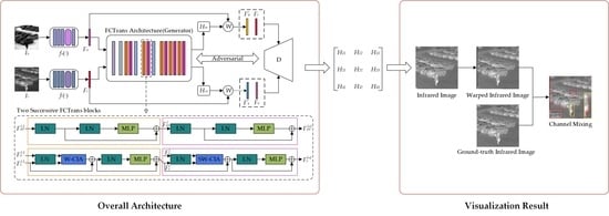
Graphical Abstract

1. Introduction

With the development of 6G Space–Air–Ground Integrated Network (6G SAGIN) [1] technology, distributed intelligent-assisted sensing, communication, and computing have become important aspects of future communication networks. This provides the possibility for more extensive perception, real-time transmission, and the real-time computation and analysis of data. Smart sensors capture information from various modalities, such as visible images and infrared images, and then transmit this information in real time to edge computing [2,3,4] devices for perception computational solving. The registration techniques of infrared and visible images can provide highly accurate perceptual images, which support more effective perceptual computations and applications, such as image fusion [5,6], target tracking [7,8], semantic segmentation [9], surveillance [10], and the Internet of Vehicles [11]. In addition, image registration techniques have received extensive attention in other interdisciplinary fields. Using various remote sensing techniques, Shugar et al. [12] effectively chronicled substantial rock and ice avalanche hazards in Chamoli, Himalayas, India. Their research emphasized the importance of accurate registration and data integration from multiple sources. Muhuri et al. [13] achieved high accuracy through accurate synthetic aperture radar (SAR) image sequence registration in estimating glacier surface velocities. Schmah et al. [14] compared computational methods in longitudinal fMRI studies, where accurate image registration is crucial. These studies show that image registration technology is vital in natural disaster monitoring, glacier movement tracking, and neuroimaging. In this context, an accurate homography estimation method is crucial.
Homography estimation, as an auxiliary perception technique, is widely used in the registration of infrared and visible images to further enhance the environmental perception capability of 6G SAGINs [15]. It not only provides real-time and accurate perception information in a distributed environment but can also be closely integrated with communication and computation to assist the network in achieving more efficient resource scheduling and decision-making. Due to the significant differences between infrared and visible images in terms of imaging principles, spectral range, and contrast, it is extremely challenging to directly estimate the homography matrix between them [16].

1.1. Related Studies

A homography matrix is a two-dimensional geometric transformation describing the projection relationship between two planes [17,18]. The traditional homography estimation method mainly includes the following key steps: feature extraction, feature matching, and solving the direct linear transform (DLT) [19] with outlier rejection. In the feature extraction stage, feature extraction algorithms are used to find feature points with stability and saliency in two images, such as Scale Invariant Feature Transform (SIFT) [20], Speeded Up Robust Features (SURFs) [21], Oriented FAST and Rotated BRIEF (ORB) [22], Binary Robust Invariant Scalable Keypoints (BRISK) [23], Accelerated-KAZE (AKAZE) [24], KAZE [25], Locality Preserving Matching (LPM) [26], Grid-Based Motion Statistics (GMS) [27], Boosted Efficient Binary Local Image Descriptor (BEBLID) [28], Learned Invariant Feature Transform (LIFT) [29], SuperPoint [30], Second-Order Similarity Network (SOSNet) [31], and Order-Aware Networks (OANs) [32]. Meanwhile, some recent studies [33,34,35] have performed a comparative analysis of detectors and feature descriptors in image registration, providing a more comprehensive reference for the selection of feature extraction algorithms. Next, feature matching is achieved by computing the similarity between feature descriptors. Some incorrect matching pairs may occur in this process; therefore, robust estimation algorithms (e.g., Random Sample Consensus (RANSAC) [36], Marginalizing Sample Consensus (MAGSAC) [37], and MAGSAC++ [38]) are needed to reject outliers and utilize DLT [19] to solve the homography. However, infrared and visible images have significant imaging differences. This may lead to limited keypoint stability, descriptor matching accuracy, and outlier handling ability during homography estimation, which affects the accuracy of the homography matrix.
In recent years, the emergence of deep learning technology has provided a new perspective to solve this problem. Deep learning-based homography estimation can be divided into supervised and unsupervised methods. Supervised methods [39,40,41] require many paired images and homography matrix labels. However, obtaining many accurate homography matrix labels can be challenging, especially in complex scenes. Shao et al. [41] utilized cross-attention to compute the correlation between different images. However, they used pixels as the basic unit to calculate attention, which are susceptible to modal differences. Unlike supervised methods, unsupervised methods do not rely on explicit homography matrix labels but perform unsupervised training by designing a loss function. Nguyen et al. [42] proposed an unsupervised deep homography estimation method that guides the network to learn the correct homography matrix through photometric loss. The method exhibited difficulties with convergence during training due to the significant grayscale difference between infrared and visible images [43,44,45,46,47], usually cascading the image pairs themselves or their feature maps in channels and then feeding them into a regression network to obtain the homography matrix. Such methods learn the associations and dependencies between the two features through regression networks to implicitly guide feature matching. Due to the significant feature differences between infrared and visible images, implicit feature matching may have difficulty accurately capturing feature correspondence between the two modal images, thus affecting the performance of homography estimation. Moreover, channel cascading may lead to feature distortion, occlusion, or interference, making matching difficult and less interpretable. In addition, Refs. [44,45] adopted the concept of homography flow to estimate homography. Their significant grayscale and contrast differences for infrared and visible images tend to lead to unstable homography flow, making it difficult for the network to converge. Although a self-attention mechanism has been used to capture the correspondence between features [45], it still faces significant difficulties in feature matching on the feature map after channel cascading.
In addition, methods based on the Swin Transformer [48] have attracted researchers’ attention. The Swin Transformer [48] is a novel visual transformer architecture that has achieved remarkable results in various computer vision tasks. Its main innovation is to replace the global self-attention mechanism in the traditional transformer with local self-attention, thus reducing computational complexity and improving computational efficiency. Huo et al. [49] proposed a homography estimation model based on the Swin Transformer. This model uses the Swin Transformer [48] to obtain a multi-level feature pyramid of image pairs and then uses the features of different levels in the subsequent homography estimation from coarse to fine. However, the Swin Transformer [48] in this model is only used for deep feature extraction.

1.2. Contribution

To solve the problems of difficult feature correspondence capture, difficult feature matching, and poor interpretability in regression networks, we propose a new feature correlation transformer, called FCTrans, for the homography estimation of infrared and visible images. Inspired by the Swin Transformer [48], we employed a similar structure to explicitly guide feature matching. We achieved explicit feature matching by computing the correlation between infrared and visible images (one is the source image; the other is the target image) in the feature patch unit within the window instead of in the pixel unit and then derived a homography matrix, as shown in Figure 1. Specifically, we first propose a feature patch, a basic unit for computing correlations, to better cope with the modal differences between infrared and visible images. Second, we propose a cross-image attention mechanism to calculate the correlation between source and target images to effectively establish feature correspondence between different modal images. The method finds the correlation between source and target images in a window in the unit of the feature patch, thus projecting the source image to the target image in the feature dimension. However, infrared and visible images have significant pixel grayscale differences and weak image correlation. This may result in very small attention weights during the training process, which makes it difficult to effectively capture the relationship between features. To address this problem, we propose a method called feature correlation loss (FCL). This approach aims to encourage the network to learn discriminative target feature mapping, which we call the projected target feature map. Then, we use the projected target feature map and the unprojected target feature map to obtain the homography matrix, thus converting the homography estimation problem between multi-source images into a problem between single-source images. Compared with previous methods, FCTrans explicitly guides feature matching by computing the correlation between infrared and visible images with a feature patch as the basic unit; additionally, it is more interpretable.
The contributions of this paper are summarized as follows:
  • We propose a new transformer structure: the feature correlation transformer (FCTrans). The FCTrans can explicitly guide feature matching, thus further improving feature matching performance and interpretability.
  • We propose a new feature patch to reduce the errors introduced by imaging differences in the multi-source images themselves for homography estimation.
  • We propose a new cross-image attention mechanism to efficiently establish feature correspondence between different modal images, thus projecting the source images into the target images in the feature dimensions.
  • We propose a new feature correlation loss (FCL) to encourage the network to learn a discriminative target feature map, which can better realize mapping from the source image to the target image.
The rest of the paper is organized as follows. In Section 2, we detail the overall architecture of the FCTrans and its components and introduce the loss function of the network. In Section 3, we present some experimental results and evaluations from an ablation study performed to demonstrate the effectiveness of the proposed components. In Section 4, the proposed method is discussed. Finally, some conclusions are presented in Section 5.

2. Methods

In this section, we first provide an overview of the overall architecture of the network. Second, we further give an overview of the proposed FCTrans and introduce the architecture of cross-image attention and the feature patch in the FCTrans. Finally, we show some details of the loss function, where the proposed FCL is described in detail.

2.1. Overview

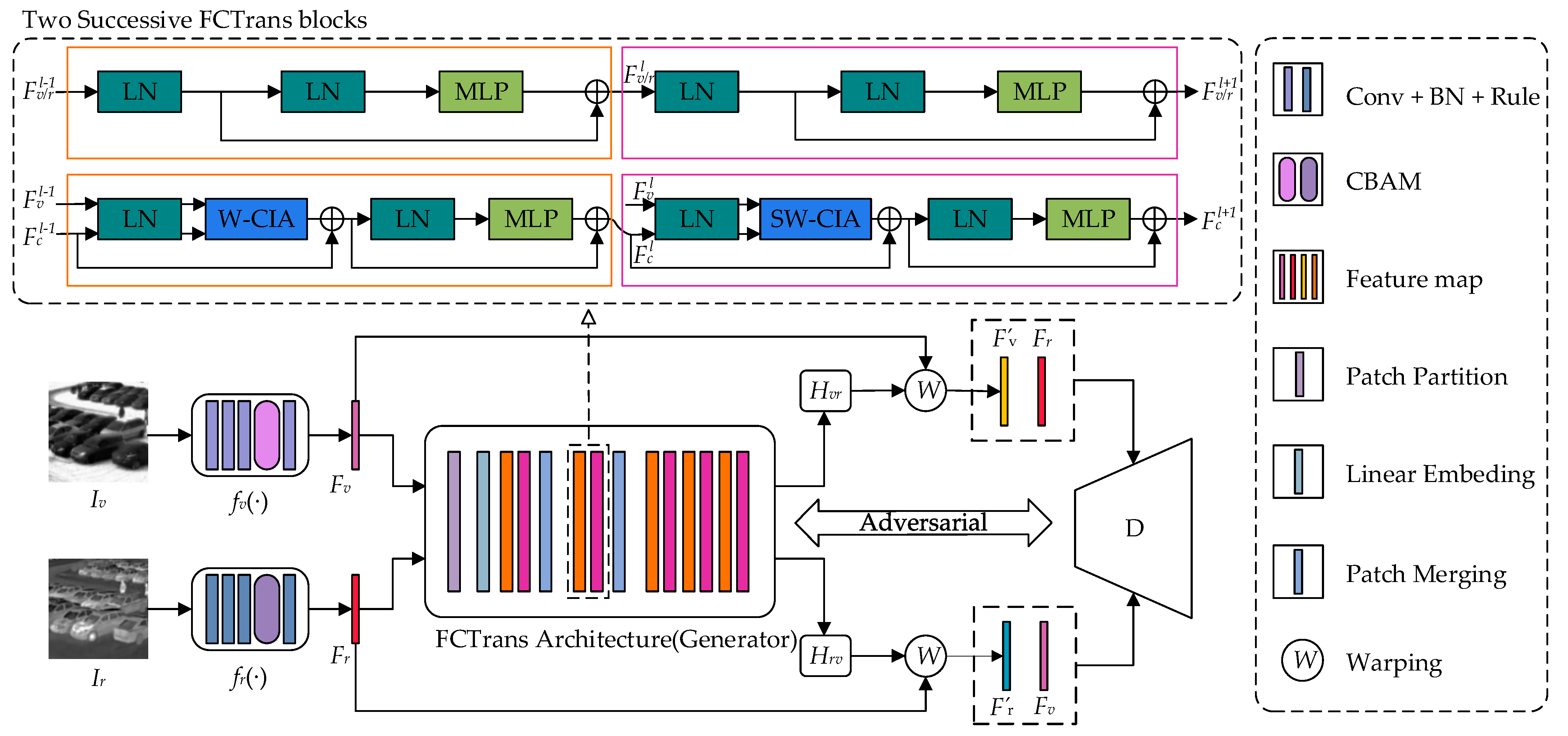
Given a pair of visible and infrared grayscale image patches, I v and I r , of size H × W × 1 as the input to the network, we produced a homography matrix from I v to I r , denoted by H v r . Similarly, we obtained the homography matrix, H r v , by exchanging the order of image patches I v and I r . The proposed model consisted of four modules: two shallow feature extraction networks (an infrared shallow feature extraction network, f r ( · ) , and a visible shallow feature extraction network, f v ( · ) ), an FCTrans generator, and a discriminator, as shown in Figure 2.
First, we converted images I v and I r into shallow feature maps F v and F r using shallow feature extraction networks f v ( · ) and f r ( · ) which did not share weights, respectively. The purpose of shallow feature extraction networks is to extract fine features that are meaningful for homography estimation from both channel and spatial dimensions. Next, we employed the FCTrans (generator) to continuously query the correlation between feature patches of the target feature map and the source feature map to explicitly guide feature matching, thus achieving mapping from the source image to the target image in the feature dimension. Then, we utilized the projected target feature map and the unprojected target feature map to obtain the homography matrix, thus converting the homography estimation problem between multi-source images into that between single-source images. Finally, we applied the homography matrix to the source image to generate the warped image and distinguish the warped image from the target image by a discriminator to further optimize the homography estimation performance. We adopted the Spatial Transformation Network (STN) [50] to implement the warping operation.
The core innovation of our method is to design a new transformer structure for homography estimation: FCTrans. By taking the feature patch as the computing unit, FCTrans constantly queries the feature correlation between infrared and visible images to explicitly guide feature matching, thus realizing mapping from the source image to the target image. We employed a method to output the homography matrix by converting the homography estimation problem of multi-source images to that of single-source images. Compared with the previous HomoMGAN [47], we deeply optimized the generator to effectively improve the performance of homography estimation.

2.2. FCTrans Structure

Previous approaches [43,44,45,46,47] usually input the features of image pairs into a regression network by channel cascading, thus implicitly learning the association between image pairs but not directly comparing their feature similarity. However, considering the significant imaging differences between infrared and visible images, this implicit featurematching method may not accurately capture the feature correspondence between the two images, thus affecting the performance of homography estimation. To solve this problem, we propose a new transformer structure (FCTrans). This structure continuously queries the correlation between a feature patch in the source feature map and all feature patches in the corresponding window of the target feature map within the window to achieve explicit feature matching, thus projecting the source image into the target image in the feature dimension. Then, we use the projected target feature map and the unprojected target feature map to obtain the homography matrix, thus converting the homography estimation problem between multi-source images into that between single-source images. The structure of the FCTrans network is shown in Figure 3.
Assuming that the source and target images are the visible image, I v , and infrared image, I r , respectively, then the corresponding source shallow feature map and target shallow feature map are F v and F r , respectively. The same assumptions are applied in the rest of this paper. First, we input F v and F r into the patch partition module and linear embedding module, respectively, to obtain the feature maps F v 0 and F r 0 of size H 2 × w 2 . Meanwhile, we made a deep copy of F r 0 to obtain F c 0 , subsequently distinguishing the projected target feature map from the unprojected target feature map.
Then, we applied two FCTrans blocks with cross-image attention to F v 0 , F r 0 , and F c 0 . In the l -th FCTrans block, we regard F v l as the query feature map (source feature map), F c l as the key/value feature map (projected target feature map), and F r l as the reference feature map (unprojected target feature map). In addition, the cross-image attention operation in each FCTrans block requires F v l 1 and F c l 1 as inputs to obtain the projected target feature map F c l , as shown at the top of Figure 2. F v l 1 and F r l 1 are regarded as the query image and the reference image, respectively, and do not need to be projected; therefore, F v l and F r l are obtained through the FCTrans block without cross-image attention, respectively. The computations in the FCTrans block are as follows:
F k l = M L P L N L N F k l 1 + L N F k l 1 , k = v , r F ^ c l = f c l 1 + F c l 1 F c l = M L P L N ( F ^ c l ) + F ^ c l
where L N ( · ) denotes the operation of the LayerNorm layer; M L P ( · ) denotes the operation of MLP; F k l indicates the feature map output by the l -th FCTrans block, where F v l , F c l , and F r l denote the source feature map, the projected target feature map and the unprojected target feature map, respectively; f c l 1 represents the feature map obtained with F v l 1 and F c l 1 as the input of cross-image attention; F ^ c l represents the output feature map of F c l 1 in the S(W)-CIA module.
To generate a hierarchical representation, we halved the feature map size and doubled the number of channels using the patch merging module. The two FCTrans blocks, together with a patch merging module, are called “Stage 1”. Similarly, “Stage 2” and “Stage 3” adopt a similar scheme. However, their FCTrans block numbers are 2 and 6, respectively, and “Stage 3” does not have a patch merging module. After three stages, each feature patch in F c 10 implies a correlation with all the feature patches in the corresponding window of the source feature map at different scales, thus achieving the goal of projecting feature information from the source image into the target image.
Finally, we concatenated F r 10 and F c 10 to build [ F r 10 , F c 10 ] and then input it to the homography prediction layer (including the LayerNorm layer, global pooling layer, and fully connected layer) to output 4 offset vectors (8 values). With the 4 offset vectors, we obtained the homography matrix, H v r , by solving the DLT [19]. We use h ( · ) to represent the whole process, i.e.:
H v r = h ( [ F r 10 , F c 10 ] )
where F r 10 represents the unprojected target feature map outputted by the 10th FCTrans block and F c 10 indicates the projected target feature map outputted by the 10th FCTrans block.
In this way, we converted the homography estimation problem for multi-source images into the homography estimation problem for single-source images, simplifying the network training. Similarly, assuming that the source and target images are infrared image I r and visible image I v , respectively, then the homography matrix H r v can be obtained based on F v 10 and F c 10 . Algorithm 1 shows some training details of the FCTrans.

2.2.1. Feature Patch

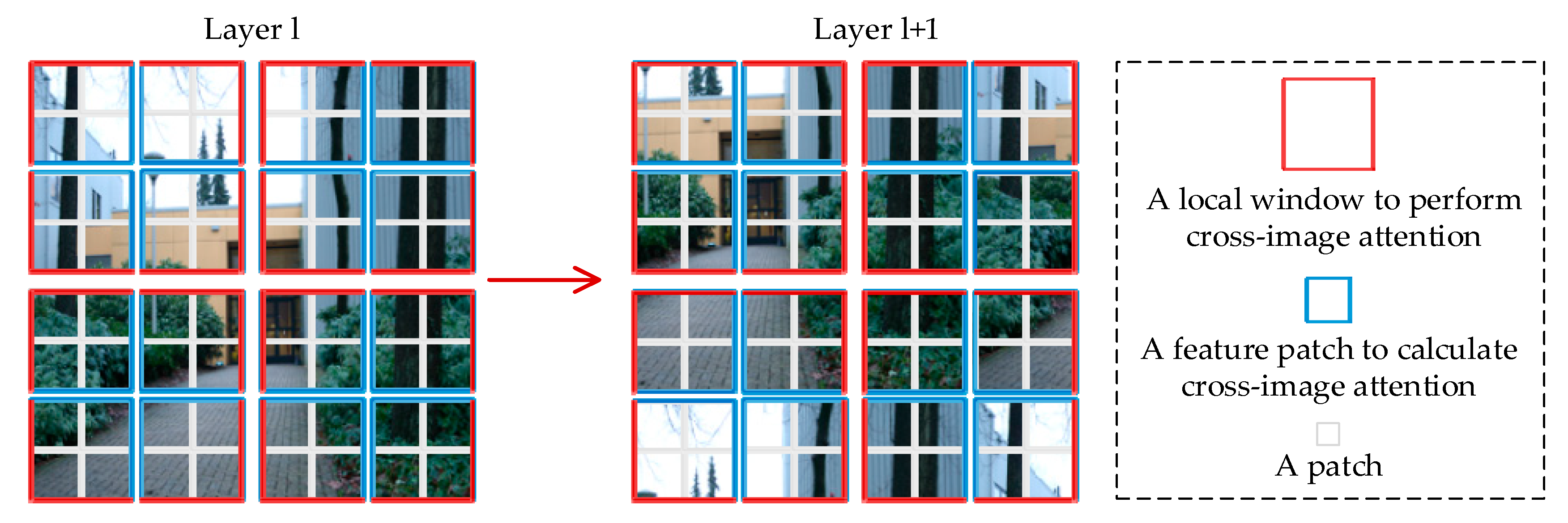
In infrared and visible image scenes, the feature-based method shows greater robustness and descriptive power compared with the pixel-based method in coping with modal differences, establishing correspondence, and handling occlusion and noise, resulting in more stable and accurate performance. In this study, we followed a similar idea, using a 2 × 2 feature patch as an image feature to participate in the attention computation instead of relying on pixels as the computational unit. Specifically, we further evenly partitioned the window of size M × M (set to 16 by default) in a non-overlapping manner and then obtained M 2 × M 2 feature patches of size 2 × 2 , as shown in Figure 4. In Figure 4, we assume that the size of the window is 4 × 4 , which results in 2 × 2 feature patches. By involving the feature patch as the basic computational unit in the attention calculation, we can capture the structural information in the image effectively while reducing the effect of modal differences on the homography estimation.
Algorithm 1: The training process of the FCTrans
Input: F v   and   F r
Output: FCL and homography matrix
Select   the   F v input to the patch partition layer and linear embedding layer: F v 0 ;
Select   the   F r input to the patch partition layer and linear embedding layer: F r 0 ;
Select   F r 0   for   deep   copy :   F c 0 ;
for n < number_of_stages do
   for k < number_of_blocks do
       Select   F v l 1   input   to   LayerNorm   layer :   L N ( F v l 1 ) ;
       Select   F r l 1   input   to   LayerNorm   layer :   L N ( F r l 1 ) ;
       Select   F c l 1   input   to   LayerNorm   layer :   L N ( F c l 1 ) ;
      Select F v l 1 and F c l 1 input to (S)W-CIA module:
y c l 1 = s o f t m a x ( Q K T d + B ) V , F ^ c l = f c l 1 + F c l 1 ;
       Select   L N ( F v l 1 ) input to LayerNorm layer and MLP:
F v l = M L P L N L N F v l 1 + L N F v l 1 ;
       Select   L N ( F r l 1 ) input to LayerNorm layer and MLP:
F r l = M L P L N L N F r l 1 + L N F r l 1 ;
      Select F ^ c l input to LayerNorm layer and MLP:
F c l = M L P L N F ^ c l + F ^ c l ;
       Calculate   and   save   loss :   L f c l ( F v l , F c l , F r l ) ;
   End
   if n < (number_of_stages-1) do
       Select   F v l input to patch merging layer;
       Select   F r l input to patch merging layer;
       Select   F c l input to patch merging layer;
end
Calculate   FCL :   L f c ( F v , F r ) = l = 1 10 L f c l ( F v l , F c l , F r l ) ;
Calculate   homography   matrix :   H v r = h ( [ F r 10 , F c 10 ] ) ;
Return:  L f c ( F v , F r ) and H v r ;

2.2.2. Cross-Image Attention

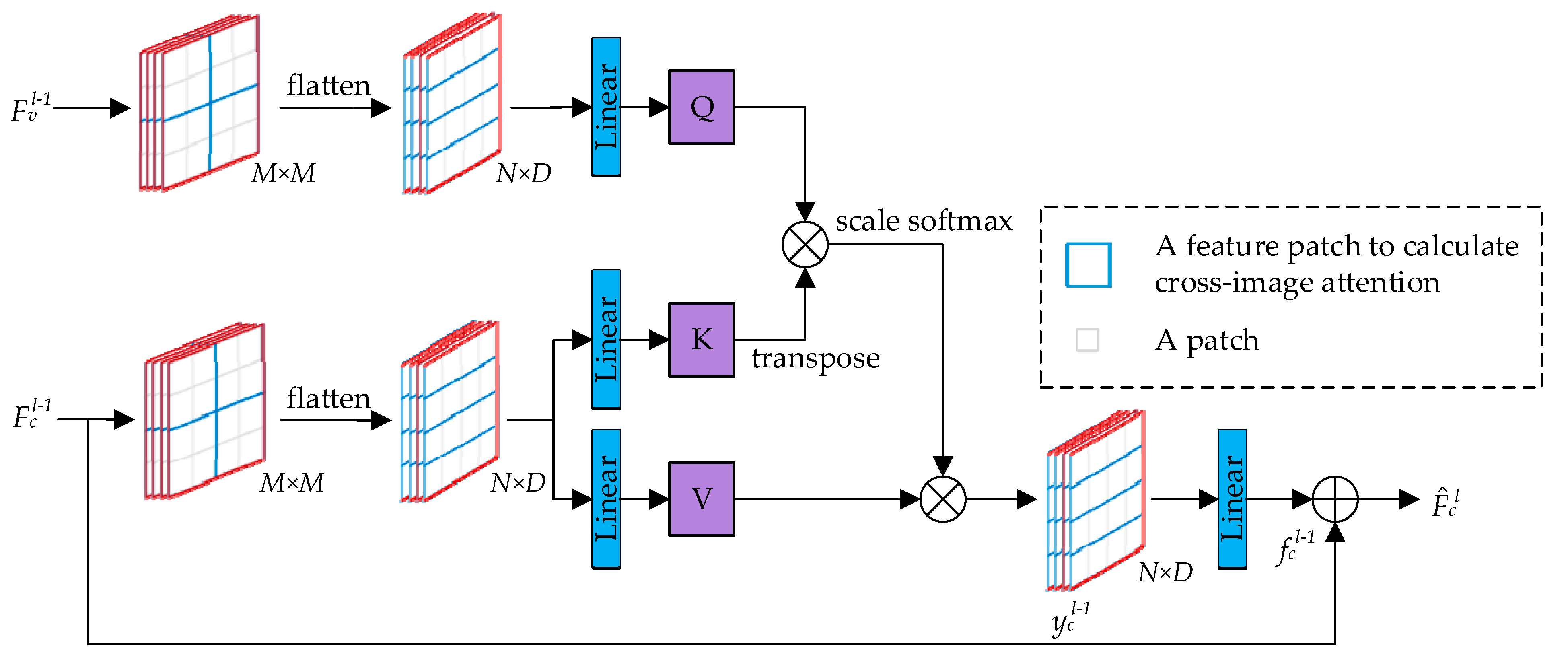
In image processing, the cross-attention mechanism [51] can help models capture dependencies and correlations between different images or images and other modal data, thus enabling effective information exchange and fusion. In this study, we borrowed a similar idea and designed a cross-image attention mechanism for the homography estimation task, as shown in Figure 5. Cross-image attention takes the feature patch as the unit and finds the correlation between a feature patch in the source feature map and all feature patches in the target feature map within the window, thus projecting the source image into the target image in the feature dimension. The dimensionality of the feature patch is small; therefore, we use single-headed attention to compute cross-image attention.
First, we take F v l 1 and F c l 1 of size H 2 k × W 2 k (where k denotes the number of stages) processed by the LayerNorm layer as the query feature map and key/value feature map. We adopt a (shifted) window partitioning scheme and a feature patch partitioning scheme to partition them into windows of size M × M containing M 2 × M 2 feature patches. Next, we flatten these windows in the feature patch dimension, thus reshaping the window size to N × D , where N denotes the number of feature patch ( M 2 × M 2 ) and D represents the number of pixels in the feature patch ( 2 × 2 ). Then, the window of F v l 1 passes through the fully connected layer to obtain the query matrix, and the window of F c l 1 passes through two different fully connected layers to obtain the key matrix and the value matrix, respectively. We compute the similarity between the query matrix and all key matrices to assign weights to each value matrix. The similarity matrix is usually computed using the dot product and then normalized to a probability distribution via the softmax function. In this way, we can query the similarity between each feature in F v l 1 (represented by feature patch) and all features in F c l 1 within the corresponding windows of F v l 1 and F c l 1 , thus achieving the effect of explicit feature matching. Finally, we multiply the value matrix and the similarity matrix to obtain the final output matrix, y c l 1 , after obtaining the weighted similarity matrix. Each feature patch in this output matrix, y c l 1 , implies the correlation between all the feature patches in the window corresponding to the source feature map, thus achieving a mapping from the source image to the target image in the feature dimension. This implementation process can be described as follows:
y c l 1 = s o f t m a x ( Q K T d + B ) V
where Q , K , and V represent the query, key, and value matrices, respectively; d stands for the Q / K dimension, which is 2 × 2 in the experiment; and B represents the relative position bias. We used a feature patch as the unit of computation; therefore, the relative positions along each axis were in the range [ M 2 + 1 , M 2 + 1 ] . We parameterized a bias matrix, B ^ R ( M 1 ) × ( M 1 ) , and the values in B were taken from B ^ . We rescaled the output matrix y c l 1 of size N × D to match the size of the original feature map, i.e., H 2 k × W 2 k . This adjustment could facilitate subsequent convolution operations or other image processing steps. In addition, we performed residual concatenation by adding the output feature map and the original feature map, F c l 1 , to obtain the feature map, F ^ c l , thus alleviating the gradient disappearance.
In particular, there may be multiple non-adjacent sub-windows in the shifted window, so the Swin Transformer [48] employs a masking mechanism to restrict attention to each window. However, we now adopt the feature patch as the basic unit of attention calculation instead of the pixel level, which makes the mask mechanism in the Swin Transformer [48] no longer applicable to our method. Considering that the size of the feature patch is 2 × 2 and the size of the window is set to be a multiple of 2 , we generate the mask adapted to our method in steps of 2 based on the mask in the Swin Transformer.

2.3. Loss Function

In this study, the generative adversarial network architecture was used to train the network, which consists of two parts: a generator (FCTrans) and a discriminator (D). The generator is responsible for generating the homography matrix to obtain the warped image. The discriminator aims to distinguish the shallow feature maps of the warped image and the target image. To train the network, we define the generator loss function and the discriminator loss function. In particular, we introduce the proposed FCL in detail in the generator loss function.

2.3.1. Loss Function of the Generator

To solve the problem of the network having difficulty adequately capturing the feature relationship between infrared and visible images, we propose a constraint called “Feature Correlation Loss” (FCL). FCL aims to minimize the distance between the projected target feature map, F c l , and the source feature map, F v l , while maintaining a large distance between the unprojected target feature map, F r l , and the source feature map, F v l . This scheme encourages the network to continuously learn the feature correlation between the projected target feature map ( F c l ) and the source feature map ( F v l ) within the window, and then continuously weight the projected target feature map under multiple stages to achieve better feature matching with the source feature map. Our FCL constraint is defined as follows:
L f c l ( F v l , F c l , F r l ) = max F c l F v l 1 F r l F v l 1 + 1,0 L f c ( F v , F r ) = l = 1 10 L f c l ( F v l , F c l , F r l )
where F v l , F c l , and F r l represent the source feature map, the projected target feature map, and the unprojected target feature map output by the l -th FCTrans block, respectively. L f c l ( F v l , F c l , F r l ) denotes the loss generated by the l -th FCTrans block. F v and F r stand for the visible shallow feature map and infrared shallow feature map, respectively. Our FCL is the sum of the losses generated by all FCTrans blocks, i.e., L f c ( F v , F r ) .
To perform unsupervised learning, we minimize three other losses in addition to constraining the FCL of FCTrans network training. The first one is the feature loss, which is used to encourage the feature maps between the warped and target images to have similar data distributions [47], written as:
L f ( I r , I v ) = m a x ( F r F v 1 F r F v 1 + 1,0 )
where I v and I r represent the visible image patch and the infrared image patch, respectively. F v and F r indicate the visible shallow feature map and the infrared shallow feature map, respectively. F r denotes the warped infrared shallow feature map obtained by warping F r with the homography matrix, H r v .
The second term is the homography loss, which is used to force H r v and H v r to be mutually inverse matrices [47], and is computed by:
L h o m = H v r H r v E 2 2
where E denotes the third-order identity matrix. H v r represents the homography matrix from I v to I r . H r v denotes the homography matrix from I r to I v .
The third term is the adversarial loss, which is used to force the feature map of the warped image to be closer to that of the target image [47], i.e.:
L a d v ( F r ) = n = 1 N ( 1 logD θ D ( F r ) )
where logD θ D ( · ) indicates the probability of the warped shallow feature map like a target shallow feature map, N represents the size of the batch, and F r stands for the warped infrared shallow feature map.
In practice, we can derive the losses L f ( I v , I r ) , L a d v ( F v ) , and L f c ( F r , F v ) by exchanging the order of image patches I v and I r . Thus, the total loss function of the generator can be written as:
L G = L f ( I r , I v ) + L f ( I v , I r ) + λ L h o m + μ ( L a d v ( F r ) ) + L a d v ( F v ) ) ) + ξ ( L f c ( F v , F r ) + L f c ( F r , F v ) )
where I v and I r stand for the visible image patch and infrared image patch, respectively. F v and F r indicate the visible shallow feature map and infrared shallow feature map, respectively. F v and F r represent the warped visible shallow feature map and the warped infrared shallow feature map, respectively. λ , μ , and ξ are the weights of each term set as 0.01, 0.005, and 0.05, respectively. We provide an analysis of parameter ξ in Appendix A.

2.3.2. Loss Function of the Discriminator

The discriminator aims to distinguish the feature maps between the warped image and the target image. According to [47], the loss between the feature map of the infrared image and the warped feature map of the visible image is calculated by:
L D ( F r , F v ) = n = 1 N ( a logD θ D ( F r ) ) + n = 1 N ( b logD θ D ( F v ) )
where F r indicates the infrared shallow feature map; F v represents the warped visible shallow feature map; N represents the size of the batch; a and b represent the labels of the shallow feature maps F r and F v , which are set as random numbers from 0.95 to 1 and 0 to 0.05, respectively; and logD θ D ( · ) indicates the probability of the warped shallow feature map to be similar to the target shallow feature map.
In practice, we can obtain the loss L D ( F v , F r ) by swapping the order of I v and I r . Thus, the total loss function of the discriminator can be defined as follows:
L D = L D ( F r , F v ) + L D ( F v , F r )
where F v and F r indicate the visible shallow feature map and infrared shallow feature map, respectively; F v and F r represent the warped visible shallow feature map and warped infrared shallow feature map, respectively.

3. Experimental Results

In this section, we first briefly introduce the synthetic benchmark dataset and the real-world dataset, and then describe some implementation details of the proposed method. Next, we briefly present the evaluation metrics used in the synthetic benchmark dataset and the real-world dataset. Second, we perform comparisons with existing methods on synthetic benchmark datasets and real-world datasets to demonstrate the performance of our method. We compare our method with traditional feature-based methods and deep-learning-based methods. The traditional feature-based methods include eight methods that are combined by four feature descriptors (SIFT [20], ORB [22], BRISK [23], and AKAZE [24]) and two outlier rejection algorithms (RANSAC [36] and MAGSAC++ [38]). The deep-learning-based methods include three methods (CADHN [43], DADHN [46], and HomoMGAN [47]). Finally, we also performed some ablation experiments to demonstrate the effectiveness of all the newly proposed components.

3.1. Dataset

We used the same synthetic benchmark dataset as Luo et al. [47] to evaluate our method. The dataset consists of unregistered infrared and visible image pairs of size 150 × 150 , which include 49,738 training pairs and 42 test pairs. In particular, the test set also includes the corresponding infrared ground-truth image I G T for each image pair, thus facilitating the presentation of channel mixing results in qualitative comparisons. Meanwhile, the test set provides four pairs of ground-truth matching corner coordinates for each pair of test images for evaluation calculation.
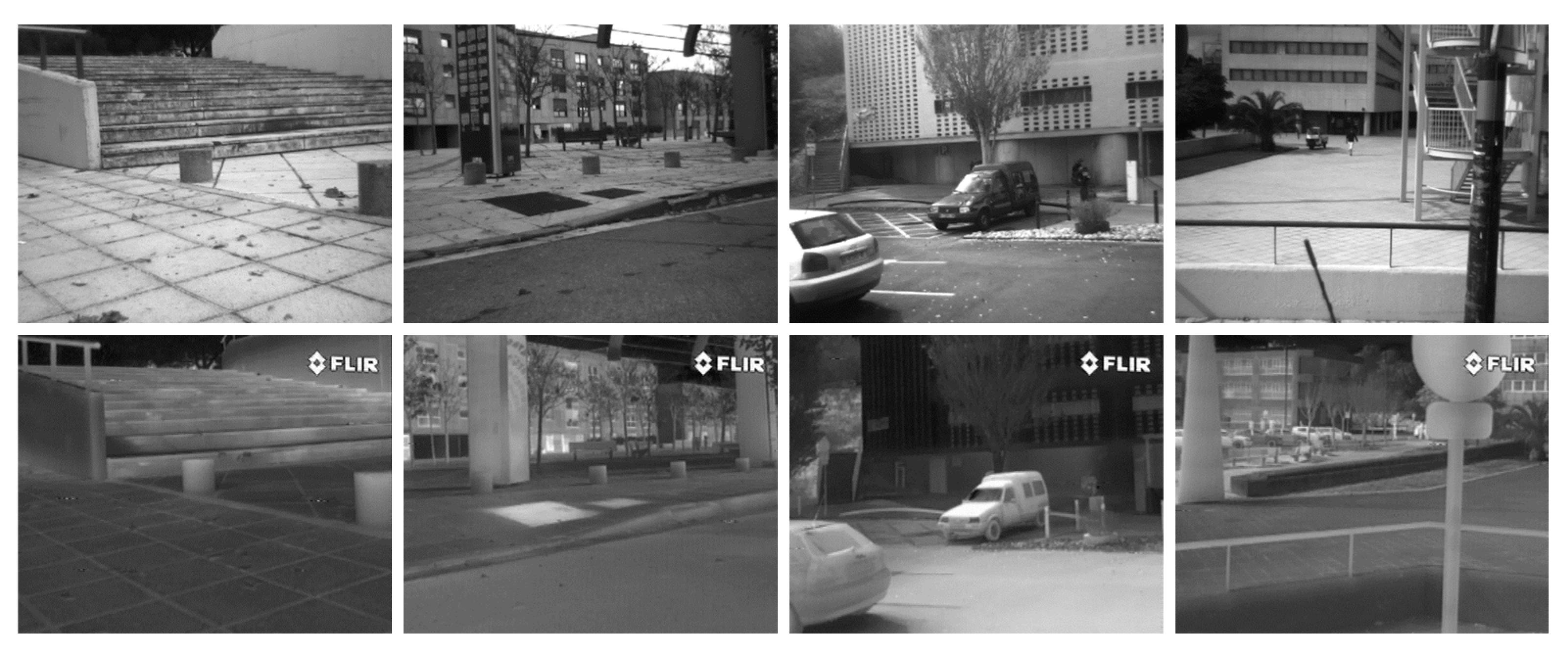
Furthermore, we utilized the CVC Multimodal Stereo Dataset [52] as our real-world dataset. This collection includes 100 pairs of long-wave infrared and visible images, primarily taken on city streets, each with a resolution of 506 × 408 . Figure 6 displays four representative image pairs from the dataset.

3.2. Implementation Details

Our experimental environment parameters are shown in Table 1. During data preprocessing, we resized the image pairs to a uniform size of 150 × 150 and then randomly cropped them to image patches of size 128 × 128 to increase the amount of data. In addition, we normalized and grayscaled the images to obtain patches I v and I r as the input of the model. Our network was trained under the PyTorch framework. To optimize the network, we employed the adaptive moment estimation (Adam) [53] optimizer with the initial value of the learning rate set to 0.0001 and adjusted by the decay strategy during the training process. All parameters of the proposed method are shown in Table 2. In each iteration of model training, we first updated the discriminator (D) parameters and then the generator (FCTrans). Its loss function is optimized by backpropagation in each iteration step. Specifically, we first utilized the generator to generate a homography matrix through which the source image is warped to a warped image. Thus, we trained the discriminator using the warped and target images. We calculated the loss function of the discriminator using Equation (8) and then updated the discriminator’s parameters by backpropagation. Next, we trained the generator. We computed the loss function of the generator using Equation (10) and updated the generator’s parameters by backpropagation. We made the network continuously tuned to the homography matrix through the adversarial game between the generator and the discriminator. Meanwhile, we periodically saved the model state during the training process for subsequent analysis and evaluation.

3.3. Evaluation Metrics

The real-world dataset lacks ground-truth matching point pairs; therefore, we employed two distinct evaluation metrics: the point matching error [43,44] for the real-world dataset and the corner error [40,41,47] for the synthetic benchmark dataset. The corner error [40,41,47] is calculated as the average l 2 distance between the corner points transformed by the estimated homography and those transformed by the ground-truth homography. A smaller value of this metric signifies a superior performance in homography estimation. The formula for computing the corner error [40,41,47] is expressed as follows:
ϱ c = 1 4 i = 1 4 x i y i 2
where x i and y i are the corner point, i , transformed by the estimated homography and the ground-truth homography, respectively.
The point matching error [43,44] is a measure of the average l 2 distance between pairs of manually labeled matching points. Lower values of this metric indicate superior performance in homography estimation. The calculation of the point matching error [43,44] is performed as follows:
L p = 1 N i = 1 N x i y i 2
where x i denotes point i transformed by the estimated homography, y i denotes the matching point corresponding to point i , and N represents the number of manually labeled matching point pairs.

3.4. Comparison on Synthetic Benchmark Datasets

We conducted qualitative and quantitative comparisons between our method and all the comparative methods on synthetic benchmark dataset to demonstrate the performance of our method.

3.4.1. Qualitative Comparison

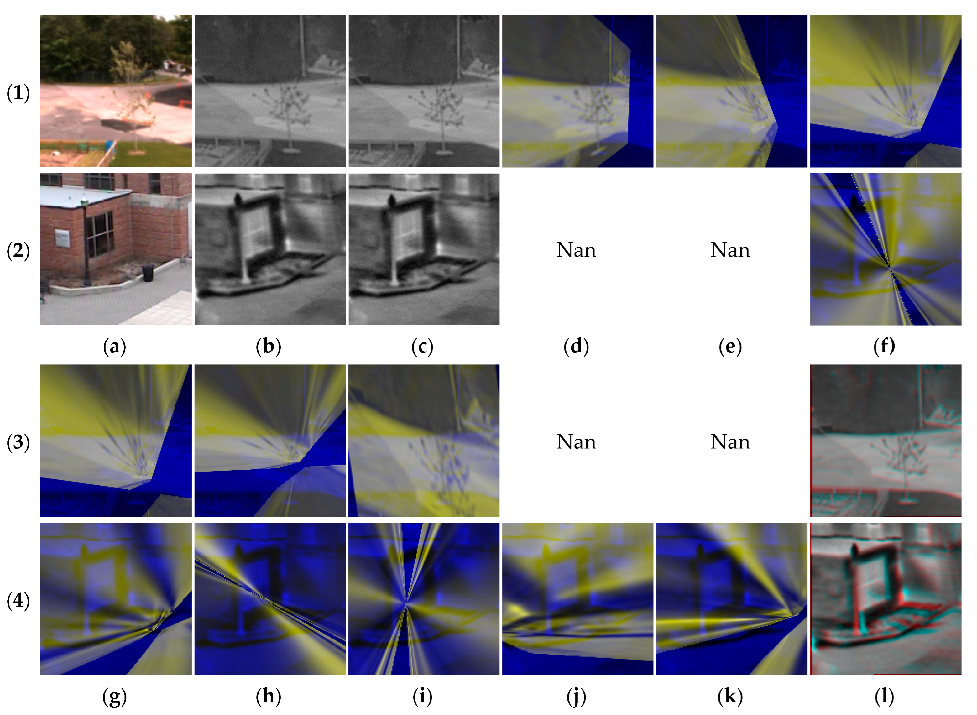
First, we compared our method with eight traditional feature-based methods, as shown in Figure 7. The traditional feature-based methods had difficulty obtaining stable feature matching in infrared and visible image scenes, which led to severe distortions in the warped image. More specifically, SIFT [20] and AKAZE [24] demonstrate algorithm failures in both examples, as shown in (2) and (3). However, our method shows better adaptability in infrared and visible image scenes, and its performance is significantly better than the traditional feature-based methods. Although SIFT [20] + RANSAC [36] in the first example is the best performer among the feature-based methods and does not exhibit severe image distortion, it still shows a large number of yellow ghosts in the ground region. These yellow ghosts indicate that the corresponding regions between the warped and ground-truth images are not aligned. However, our method shows significantly fewer ghosts in the ground region compared with the SIFT [20] + RANSAC [36] method, showing superior results. This indicates that our method has higher accuracy in processing infrared and visible image scenes.
Secondly, we compared our method with three deep learning-based methods, as shown in Figure 8. Our method exhibited higher accuracy in image alignment compared with the other methods. In addition, CHDHN [43], DADHN [46], and HomoMGAN [47] showed the different extents of green ghosting when processing door frame edges and door surface textures in (1). However, these ghosts were significantly reduced by our method, which fully illustrates its superiority. Similarly, our method achieves superior results on the alignment of cars and people in (2) compared with other deep-learning-based methods.

3.4.2. Quantitative Comparison

To demonstrate the performance of the proposed method, we performed a quantitative comparison with all other methods. We classify the testing results into three levels based on performance: easy (top 0–30%), moderate (top 30–60%), and hard (top 60–100%). We report the corner error, the overall average corner error, and the failure rate of the algorithm for the three levels in Table 3, where rows 3–10 are for the traditional feature-based methods and rows 11–13 are for the deep-learning-based methods. In particular, the failure rate in the last column of Table 3 indicates the ratio of the number of test images in which the algorithm failed against the total number of test images. I 3 × 3 in row 2 denotes the identity transformation, whose error reflects the original distance between point pairs. The “Nan” in Table 3 indicates that the corner error is not present at this level. This usually means that the method has a large number of failures in the test set; thus, no test results can be classified into this level.
As can be seen in Table 3, our method achieved the best performance at all three levels. In particular, the average corner error of our method significantly decreased from 5.06 to 4.92 compared with the suboptimal algorithm HomoMGAN [47]. Specifically, the performance of the feature-based method is significantly lower than that of the deep-learning-based method under all three levels, and all of them show algorithm failures. Meanwhile, although the average corner error of SIFT [20] + RANSAC [36] is 50.87, the average corner error of other feature-based methods is above 100. This illustrates the generally worse performance of the traditional feature-based methods. Although SIFT [20] +RANSAC [36] has the most excellent performance among all feature-based methods, it fails on most of the test images. As a result, most traditional feature-based methods in infrared and visible image scenes usually fail to extract or match enough key points, which leads to algorithm failure or poor performance and is difficult to be applied in practice.
In contrast, deep-learning-based methods can easily avoid this problem. They not only avoid algorithm failure but also significantly improve performance. CADHN [43], DADHN [46], and HomoMGAN [47] achieved excellent performance in the test images with average corner errors of 5.25, 5.08, and 5.06, respectively. However, they are guided implicitly in the regression network for feature matching, which leads to limited performance in homography estimation. In contrast, our method converts the homography estimation problem for multi-source images into a problem for single-source images by explicitly guiding feature matching, thus significantly reducing the difficulties incurred due to the large imaging differences of multi-source images for network training. As shown in Table 3, our method significantly outperforms existing deep-learning-based methods in terms of error at all three levels and overall average corner error, and the average corner error can be reduced to 4.91. This sufficiently demonstrates the superiority of explicit feature matching in our method.

3.5. Comparison on the Real-World Dataset

We performed a quantitative comparison with 11 methods on the real-world dataset to demonstrate the effectiveness of our method, as shown in Table 4. The evaluation results of the feature-based methods on the real-world dataset are similar to the results on the synthetic benchmark dataset, and both show varying degrees of algorithm failure and poor algorithm performance. In contrast, the deep-learning-based methods performed significantly better than the feature-based methods, and no algorithm failures were observed. The proposed algorithm achieves the best performance among the deep-learning-based methods; the performance of CADHN [43] and DADHN [46] is comparable with the average point matching errors of 3.46 and 3.47, respectively. Notably, our algorithm significantly improves the performance by explicitly guiding feature matching in the regression network compared to HomoMGAN [47], and the average point matching error is significantly reduced from 3.36 to 2.79. This fully illustrates the superiority of explicitly guided feature matching compared to implicitly guided feature matching.

3.6. Ablation Studies

In this section, we present the results of the ablation experiments performed on the FCTrans, feature patch, cross-image attention, and FCL and combine some visualization results to demonstrate the effectiveness of the proposed method and its components.

3.6.1. FCTrans

The proposed FCTrans is an architecture similar to the Swin Transformer [48]. To evaluate the effectiveness of FCTrans, we replaced it with the Swin Transformer [48] to serve as the backbone network of the generator; the results are shown in row 2 of Table 5. In this process, we channel-cascade the shallow features of the infrared and visible images and feed them into the Swin Transformer [48] to generate four 2D offset vectors (eight values), which, in turn, are solved by DLT [19] to obtain the homography matrix. By comparing the data in rows 2 and 6 of Table 5, we observe a significant decrease in the average corner error from 5.13 to 4.91. This result demonstrates that the proposed FCTrans can effectively improve the homography estimation performance compared with the Swin Transformer [48].

3.6.2. Feature Patch

To verify the validity of the feature patch, we removed all operations related to the feature patch from our network; the results are shown in row 3 of Table 5. Due to the removal of the feature patch, we performed the attention calculation in pixels within the window. By comparing the data in rows 3 and 6 of Table 5, our average corner error is reduced from 5.02 to 4.91. This result shows that the feature patch is more adept at capturing structural information in images, thus reducing the effect of modal differences on homography estimation.

3.6.3. Cross-Image Attention

To verify the effectiveness of cross-image attention, we used self-attention [48] to replace cross-image attention in our experiments; the results are shown in row 4 of Table 5. In this process, we channel-concatenated the shallow features of the infrared image and the visible image as the input of self-attention [48] to obtain the homography matrix. The replaced network no longer applies the FCL; therefore, we removed the operations associated with the FCL. By comparing rows 4 and 6 in Table 5, we found that the average corner error significantly decreases from 5.03 to 4.91. This is a sufficient indication that cross-image attention can effectively capture the correlation between different modal images, thus improving the homography estimation performance.

3.6.4. FCL

We removed the term of Equation (4) from Equation (8) to verify the validity of the FCL; the results are shown in row 5 of Table 5. By comparing the data in rows 5 and 6 of Table 5, we found that the average corner error was significantly reduced from 5.10 to 4.91. In addition, we visualized the attention weights of the window to further verify the validity of the FCL; the results are shown in Figure 9. As shown in the comparison of (a) and (c), the FCL allows the network to better adapt to the modal differences between infrared and visible images, thus achieving better performance in capturing inter-feature correlations. Additionally, the performance of the proposed method in (b) and (d) is slightly superior to the “ w/o. FCL”, with the average corner error reduced from 5.17 to 4.71.

4. Discussion

In this study, we proposed a feature correlation transformer method which significantly improves the accuracy of homography estimation in infrared and visible images. By introducing feature patch and cross-image attention mechanisms, our method dramatically improves the precision of feature matching. It tackles the challenges induced by the insufficient quantity and low similarity of feature points in traditional methods. Extensive experimental data demonstrate that our method significantly outperforms existing techniques in terms of both quantitative and qualitative results. However, our method also has some limitations. Firstly, although our method performs well in dealing with modality differences in infrared and visible images, it might need further optimization and adjustment when processing images in large-baseline scenarios. In future research, we aim to further improve the robustness of our method to cope with challenges in large-baseline scenarios. Moreover, we will further explore combining our method with other perception computing tasks to enhance the perception capability of 6G SAGINs.

5. Conclusions

In this study, we have proposed a feature correlation transformer method for the homography estimation of infrared and visible images, aiming to provide a higher-accuracy environment-assisted perception technique for 6G SAGINs. Compared with previous methods, our approach explicitly guides feature matching in a regression network, thus enabling the mapping of source-to-target images in the feature dimension. With this strategy, we converted the homography estimation problem between multi-source images into that of single-source images, which significantly improved the homography estimation performance. Specifically, we innovatively designed a feature patch as the basic unit for correlation queries to better handle modal differences. Moreover, we designed a cross-image attention mechanism that enabled mapping the source-to-target images in feature dimensions. In addition, we have proposed a feature correlation loss (FCL) constraint that further optimizes the mapping from source-to-target images. Extensive experimental results demonstrated the effectiveness of all the newly proposed components; our performance is significantly superior to existing methods. Nevertheless, the performance of our method may be limited in large-baseline infrared and visible image scenarios. Therefore, we intend to further explore the problem of homography estimation in large-baseline situations in future studies in order to further enhance the scene perception capability of the 6G SAGIN.

Author Contributions

Conceptualization, X.W. and Y.L.; methodology, X.W. and Y.L.; software, X.W.; validation, X.W. and Y.L.; formal analysis, X.W., Y.L., Q.F., Y.R., and C.S.; investigation, Y.W., Z.H. and Y.H.; resources, Y.L.; data curation, Y.L.; writing—original draft preparation, X.W. and Y.L.; writing—review and editing, X.W., Y.L., Y.R. and C.S.; visualization, X.W. and Y.L.; supervision, Y.W., Z.H., and Y.H.; project administration, Y.W., Z.H., and Y.H.; funding acquisition, Y.L. and Q.F. All authors have read and agreed to the published version of the manuscript.

Funding

This research was funded in part by the National Key R&D Program of China (program no. 2021YFF0603904), in part by the Science and Technology Plan Project of Sichuan Province (program no. 2022YFG0027), and in part by the Fundamental Research Funds for the Central Universities (program no. ZJ2022-004, and no. ZHMH2022-006).

Data Availability Statement

Not applicable.

Acknowledgments

We sincerely thank the authors of SIFT, ORB, KAZE, BRISK, AKAZE, and CADHN for providing their algorithm codes to facilitate the comparative experiment. Meanwhile, we would like to thank the anonymous reviewers for their valuable suggestions, which were of great help in improving the quality of this paper.

Conflicts of Interest

The authors declare no conflict of interest.

Abbreviations

The following abbreviations are used in this manuscript:
6G SAGIN6G Space–Air–Ground Integrated Network
SARSynthetic Aperture Radar
DLTDirect Linear Transformation
FCLFeature Correlation Loss
SIFTScale Invariant Feature Transform
SURFSpeeded Up Robust Features
ORBOriented FAST and Rotated BRIEF
BRISKBinary Robust Invariant Scalable Keypoints
AKAZEAccelerated-KAZE
LPMLocality Preserving Matching
GMSGrid-Based Motion Statistics
BEBLIDBoosted Efficient Binary Local Image Descriptor
LIFTLearned Invariant Feature Transform
SOSNetSecond-Order Similarity Network
OANOrder-Aware Networks
RANSACRandom Sample Consensus
MAGSACMarginalizing Sample Consensus
W-CIACross-image attention with regular window
SW-CIACross-image attention with shifted window
STNSpatial Transformation Network
AdamAdaptive Moment Estimation

Appendix A. Dependency on ξ

The values of the λ , μ , a , and b   parameters in the loss function are with reference to HomoMGAN [47]; therefore, we only analyzed the ξ parameter. The evaluation results for the ξ parameter at different values is shown in Table A1, thus presenting our fine-tuning process. The best performance of the homography estimation was obtained for a value of 0.05 for the ξ parameter.
Table A1. Dependency on ξ ; the results of the evaluation of parameter ξ at different values.
ξ EasyModerateHardAverage
0.0014.155.286.265.33
0.0053.754.705.944.91
0.013.834.886.065.03

References

  1. Liao, Z.; Chen, C.; Ju, Y.; He, C.; Jiang, J.; Pei, Q. Multi-Controller Deployment in SDN-Enabled 6G Space–Air–Ground Integrated Network. Remote Sens. 2022, 14, 1076. [Google Scholar] [CrossRef]
  2. Chen, C.; Wang, C.; Liu, B.; He, C.; Cong, L.; Wan, S. Edge Intelligence Empowered Vehicle Detection and Image Segmentation for Autonomous Vehicles. IEEE Trans. Intell. Transp. Syst. 2023, 1–12. [Google Scholar] [CrossRef]
  3. Ju, Y.; Chen, Y.; Cao, Z.; Liu, L.; Pei, Q.; Xiao, M.; Ota, K.; Dong, M.; Leung, V.C. Joint Secure Offloading and Resource Allocation for Vehicular Edge Computing Network: A Multi-Agent Deep Reinforcement Learning Approach. IEEE Trans. Intell. Transp. Syst. 2023, 24, 5555–5569. [Google Scholar] [CrossRef]
  4. Chen, C.; Yao, G.; Liu, L.; Pei, Q.; Song, H.; Dustdar, S. A Cooperative Vehicle-Infrastructure System for Road Hazards Detection With Edge Intelligence. IEEE Trans. Intell. Transp. Syst. 2023, 24, 5186–5198. [Google Scholar] [CrossRef]
  5. Xu, H.; Ma, J.; Yuan, J.; Le, Z.; Liu, W. Rfnet: Unsupervised network for mutually reinforcing multi-modal image registration and fusion. In Proceedings of the IEEE/CVF Conference on Computer Vision and Pattern Recognition, New Orleans, LA, USA, 19–24 June 2022; pp. 19679–19688. [Google Scholar]
  6. Li, L.; Han, L.; Ding, M.; Cao, H. Multimodal image fusion framework for end-to-end remote sensing image registration. IEEE Trans. Geosci. Remote Sens. 2023, 61, 1–14. [Google Scholar] [CrossRef]
  7. LaHaye, N.; Ott, J.; Garay, M.J.; El-Askary, H.M.; Linstead, E. Multi-modal object tracking and image fusion with unsupervised deep learning. IEEE J. Sel. Top. Appl. Earth Observ. Remote Sens. 2019, 12, 3056–3066. [Google Scholar] [CrossRef]
  8. Zhang, X.; Ye, P.; Leung, H.; Gong, K.; Xiao, G. Object fusion tracking based on visible and infrared images: A comprehensive review. Inf. Fusion 2020, 63, 166–187. [Google Scholar] [CrossRef]
  9. Lv, N.; Zhang, Z.; Li, C.; Deng, J.; Su, T.; Chen, C.; Zhou, Y. A hybrid-attention semantic segmentation network for remote sensing interpretation in land-use surveillance. Int. J. Mach. Learn. Cybern. 2023, 14, 395–406. [Google Scholar] [CrossRef]
  10. Drouin, M.A.; Fournier, J. Infrared and Visible Image Registration for Airborne Camera Systems. In Proceedings of the 2022 IEEE International Conference on Image Processing (ICIP), Bordeaux, France, 16–19 October 2022; pp. 951–955. [Google Scholar]
  11. Jia, F.; Chen, C.; Li, J.; Chen, L.; Li, N. A BUS-aided RSU access scheme based on SDN and evolutionary game in the Internet of Vehicle. Int. J. Commun. Syst. 2022, 35, e3932. [Google Scholar] [CrossRef]
  12. Shugar, D.H.; Jacquemart, M.; Shean, D.; Bhushan, S.; Upadhyay, K.; Sattar, A.; Schwanghart, W.; Mcbride, S.; Van Wyk de Vries, M.; Mergili, M.; et al. A massive rock and ice avalanche caused the 2021 disaster at Chamoli, Indian Himalaya. Science 2021, 373, 300–306. [Google Scholar] [CrossRef]
  13. Muhuri, A.; Bhattacharya, A.; Natsuaki, R.; Hirose, A. Glacier surface velocity estimation using stokes vector correlation. In Proceedings of the 2015 IEEE 5th Asia-Pacific Conference on Synthetic Aperture Radar (APSAR), Singapore, 29 October 2015; pp. 606–609. [Google Scholar]
  14. Schmah, T.; Yourganov, G.; Zemel, R.S.; Hinton, G.E.; Small, S.L.; Strother, S.C. Comparing classification methods for longitudinal fMRI studies. Neural Comput. 2010, 22, 2729–2762. [Google Scholar] [CrossRef] [PubMed]
  15. Gao, X.; Shi, Y.; Zhu, Q.; Fu, Q.; Wu, Y. Infrared and Visible Image Fusion with Deep Neural Network in Enhanced Flight Vision System. Remote Sens. 2022, 14, 2789. [Google Scholar] [CrossRef]
  16. Hu, H.; Li, B.; Yang, W.; Wen, C.-Y. A Novel Multispectral Line Segment Matching Method Based on Phase Congruency and Multiple Local Homographies. Remote Sens. 2022, 14, 3857. [Google Scholar] [CrossRef]
  17. Nie, L.; Lin, C.; Liao, K.; Liu, S.; Zhao, Y. Depth-Aware Multi-Grid Deep Homography Estimation with Contextual Correlation. arXiv 2021, arXiv:2107.02524. [Google Scholar] [CrossRef]
  18. Li, M.; Liu, J.; Yang, H.; Song, W.; Yu, Z. Structured Light 3D Reconstruction System Based on a Stereo Calibration Plate. Symmetry 2020, 12, 772. [Google Scholar] [CrossRef]
  19. Hartley, R.; Zisserman, A. Multiple View Geometry in Computer Vision; Cambridge University Press: Cambridge, UK, 2003. [Google Scholar]
  20. Lowe, D.G. Distinctive image features from scale-invariant keypoints. Int. J. Comput. Vis. 2004, 60, 91–110. [Google Scholar] [CrossRef]
  21. Bay, H.; Tuytelaars, T.; Gool, L.V. Surf: Speeded Up Robust Features. In Proceedings of the European Conference on Computer Vision, Graz, Austria, 7–13 May 2006; pp. 404–417. [Google Scholar]
  22. Rublee, E.; Rabaud, V.; Konolige, K.; Bradski, G. ORB: An Efficient Alternative to SIFT or SURF. In Proceedings of the 2011 International Conference on Computer Vision, Barcelona, Spain, 6–13 November 2011; pp. 2564–2571. [Google Scholar]
  23. Leutenegger, S.; Chli, M.; Siegwart, R.Y. BRISK: Binary Robust Invariant Scalable Keypoints. In Proceedings of the 2011 International Conference on Computer Vision, Barcelona, Spain, 6–13 November 2011; pp. 2548–2555. [Google Scholar]
  24. Alcantarilla, P.F.; Solutions, T. Fast explicit diffusion for accelerated features in nonlinear scale spaces. IEEE Trans. Patt. Anal. Mach. Intell 2011, 34, 1281–1298. [Google Scholar]
  25. Alcantarilla, P.F.; Bartoli, A.; Davison, A.J. KAZE Features. In Proceedings of the Computer Vision–ECCV 2012: 12th European Conference on Computer Vision, Florence, Italy, 7–13 October 2012; pp. 214–227. [Google Scholar]
  26. Ma, J.; Zhao, J.; Jiang, J.; Zhou, H.; Guo, X. Locality preserving matching. Int. J. Comput. Vis. 2019, 127, 512–531. [Google Scholar] [CrossRef]
  27. Bian, J.W.; Lin, W.Y.; Matsushita, Y.; Yeung, S.K.; Nguyen, T.D.; Cheng, M.M. Gms: Grid-Based Motion Statistics for Fast, Ultra-Robust Feature Correspondence. In Proceedings of the IEEE Conference on Computer Vision and Pattern Recognition, Honolulu, HI, USA, 21–26 July 2017; pp. 4181–4190. [Google Scholar]
  28. Suárez, I.; Sfeir, G.; Buenaposada, J.M.; Baumela, L. BEBLID: Boosted efficient binary local image descriptor. Pattern Recognit. Lett. 2020, 133, 366–372. [Google Scholar] [CrossRef]
  29. Yi, K.M.; Trulls, E.; Lepetit, V.; Fua, P. Lift: Learned Invariant Feature Transform. In Proceedings of the Computer Vision–ECCV 2016: 14th European Conference, Amsterdam, The Netherlands, 10–16 October 2016; pp. 467–483. [Google Scholar]
  30. DeTone, D.; Malisiewicz, T.; Rabinovich, A. Superpoint: Self-Supervised Interest Point Detection and Description. In Proceedings of the IEEE Conference on Computer Vision and Pattern Recognition Workshops, Salt Lake City, UT, USA, 18–22 June 2018; pp. 224–236. [Google Scholar]
  31. Tian, Y.; Yu, X.; Fan, B.; Wu, F.; Heijnen, H.; Balntas, V. Sosnet: Second Order Similarity Regularization for Local Descriptor Learning. In Proceedings of the IEEE/CVF Conference on Computer Vision and Pattern Recognition, Long Beach, CA, USA, 15–20 June 2019; pp. 11016–11025. [Google Scholar]
  32. Zhang, J.; Sun, D.; Luo, Z.; Yao, A.; Zhou, L.; Shen, T.; Chen, Y.; Quan, L.; Liao, H. Learning Two-View Correspondences and Geometry Using Order-Aware Network. In Proceedings of the IEEE/CVF International Conference on Computer Vision, Seoul, Republic of Korea, 27 October–2 November 2019; pp. 5845–5854. [Google Scholar]
  33. Mukherjee, D.; Jonathan Wu, Q.M.; Wang, G. A comparative experimental study of image feature detectors and descriptors. Mach. Vis. Appl. 2015, 26, 443–466. [Google Scholar] [CrossRef]
  34. Forero, M.G.; Mambuscay, C.L.; Monroy, M.F.; Miranda, S.L.; Méndez, D.; Valencia, M.O.; Gomez Selvaraj, M. Comparative Analysis of Detectors and Feature Descriptors for Multispectral Image Matching in Rice Crops. Plants 2021, 10, 1791. [Google Scholar] [CrossRef] [PubMed]
  35. Sharma, S.K.; Jain, K.; Shukla, A.K. A Comparative Analysis of Feature Detectors and Descriptors for Image Stitching. Appl. Sci. 2023, 13, 6015. [Google Scholar] [CrossRef]
  36. Fischler, M.A.; Bolles, R.C. Random sample consensus: A paradigm for model fitting with applications to image analysis and automated cartography. Commun. ACM 1981, 24, 381–395. [Google Scholar] [CrossRef]
  37. Barath, D.; Matas, J.; Noskova, J. MAGSAC: Marginalizing Sample Consensus. In Proceedings of the IEEE/CVF Conference on Computer Vision and Pattern Recognition, Long Beach, CA, USA, 15–20 June 2019; pp. 10197–10205. [Google Scholar]
  38. Barath, D.; Noskova, J.; Ivashechkin, M.; Matas, J. MAGSAC++, a Fast, Reliable and Accurate Robust Estimator. In Proceedings of the IEEE/CVF Conference on Computer Vision and Pattern Recognition, Seattle, WA, USA, 14–19 June 2020; pp. 1304–1312. [Google Scholar]
  39. DeTone, D.; Malisiewicz, T.; Rabinovich, A. Deep image homography estimation. arXiv 2016, arXiv:1606.03798. [Google Scholar]
  40. Le, H.; Liu, F.; Zhang, S.; Agarwala, A. Deep Homography Estimation for Dynamic Scenes. In Proceedings of the IEEE/CVF Conference on Computer Vision and Pattern Recognition, Seattle, WA, USA, 14–19 June 2020; pp. 7652–7661. [Google Scholar]
  41. Shao, R.; Wu, G.; Zhou, Y.; Fu, Y.; Fang, L.; Liu, Y. Localtrans: A Multiscale Local Transformer Network for Cross-Resolution Homography Estimation. In Proceedings of the IEEE/CVF International Conference on Computer Vision, Montreal, QC, Canada, 10–17 October 2021; pp. 14890–14899. [Google Scholar]
  42. Nguyen, T.; Chen, S.W.; Shivakumar, S.S.; Taylor, C.J.; Kumar, V. Unsupervised deep homography: A fast and robust homography estimation model. IEEE Robot. Autom. Lett. 2018, 3, 2346–2353. [Google Scholar] [CrossRef] [Green Version]
  43. Zhang, J.; Wang, C.; Liu, S.; Jia, L.; Ye, N.; Wang, J.; Zhou, J.; Sun, J. Content-Aware Unsupervised Deep Homography Estimation. In Proceedings of the Computer Vision–ECCV 2020: 16th European Conference, Glasgow, UK, 23–28 August 2020; pp. 653–669. [Google Scholar]
  44. Ye, N.; Wang, C.; Fan, H.; Liu, S. Motion Basis Learning for Unsupervised Deep Homography Estimation with Subspace Projection. In Proceedings of the IEEE/CVF International Conference on Computer Vision, Montreal, QC, Canada, 10–17 October 2021; pp. 13117–13125. [Google Scholar]
  45. Hong, M.; Lu, Y.; Ye, N.; Lin, C.; Zhao, Q.; Liu, S. Unsupervised Homography Estimation with Coplanarity-Aware GAN. In Proceedings of the IEEE/CVF Conference on Computer Vision and Pattern Recognition, New Orleans, LA, USA, 19–24 June 2022; pp. 17663–17672. [Google Scholar]
  46. Luo, Y.; Wang, X.; Wu, Y.; Shu, C. Detail-Aware Deep Homography Estimation for Infrared and Visible Image. Electronics 2022, 11, 4185. [Google Scholar] [CrossRef]
  47. Luo, Y.; Wang, X.; Wu, Y.; Shu, C. Infrared and Visible Image Homography Estimation Using Multiscale Generative Adversarial Network. Electronics 2023, 12, 788. [Google Scholar] [CrossRef]
  48. Liu, Z.; Lin, Y.; Cao, Y.; Hu, H.; Wei, Y.; Zhang, Z.; Lin, S.; Guo, B. Swin transformer: Hierarchical vision transformer using shifted windows. In Proceedings of the IEEE/CVF International Conference on Computer Vision, Montreal, QC, Canada, 10–17 October 2021; pp. 10012–10022. [Google Scholar]
  49. Huo, M.; Zhang, Z.; Yang, X. AbHE: All Attention-based Homography Estimation. arXiv 2022, arXiv:2212.03029. [Google Scholar]
  50. Jaderberg, M.; Simonyan, K.; Zisserman, A.; Kavukcuoglu, K. Spatial Transformer Networks. In Proceedings of the Advances in Neural Information Processing Systems, Montreal, QC, Canada, 7–12 December 2015; pp. 2017–2025. [Google Scholar]
  51. Vaswani, A.; Shazeer, N.; Parmar, N.; Uszkoreit, J.; Jones, L.; Gomez, A.N.; Kaiser, L.; Polosukhin, I. Attention Is All You Need. In Advances in Neural Information Processing Systems 30; Massachusetts Institute of Technology: Cambridge, MA, USA, 2017. [Google Scholar]
  52. Aguilera, C.; Barrera, F.; Lumbreras, F.; Sappa, A.D.; Toledo, R. Multispectral Image Feature Points. Sensors 2012, 12, 12661–12672. [Google Scholar] [CrossRef] [Green Version]
  53. Kingma, D.P.; Ba, J. Adam: A method for stochastic optimization. arXiv 2014, arXiv:1412.6980. [Google Scholar]
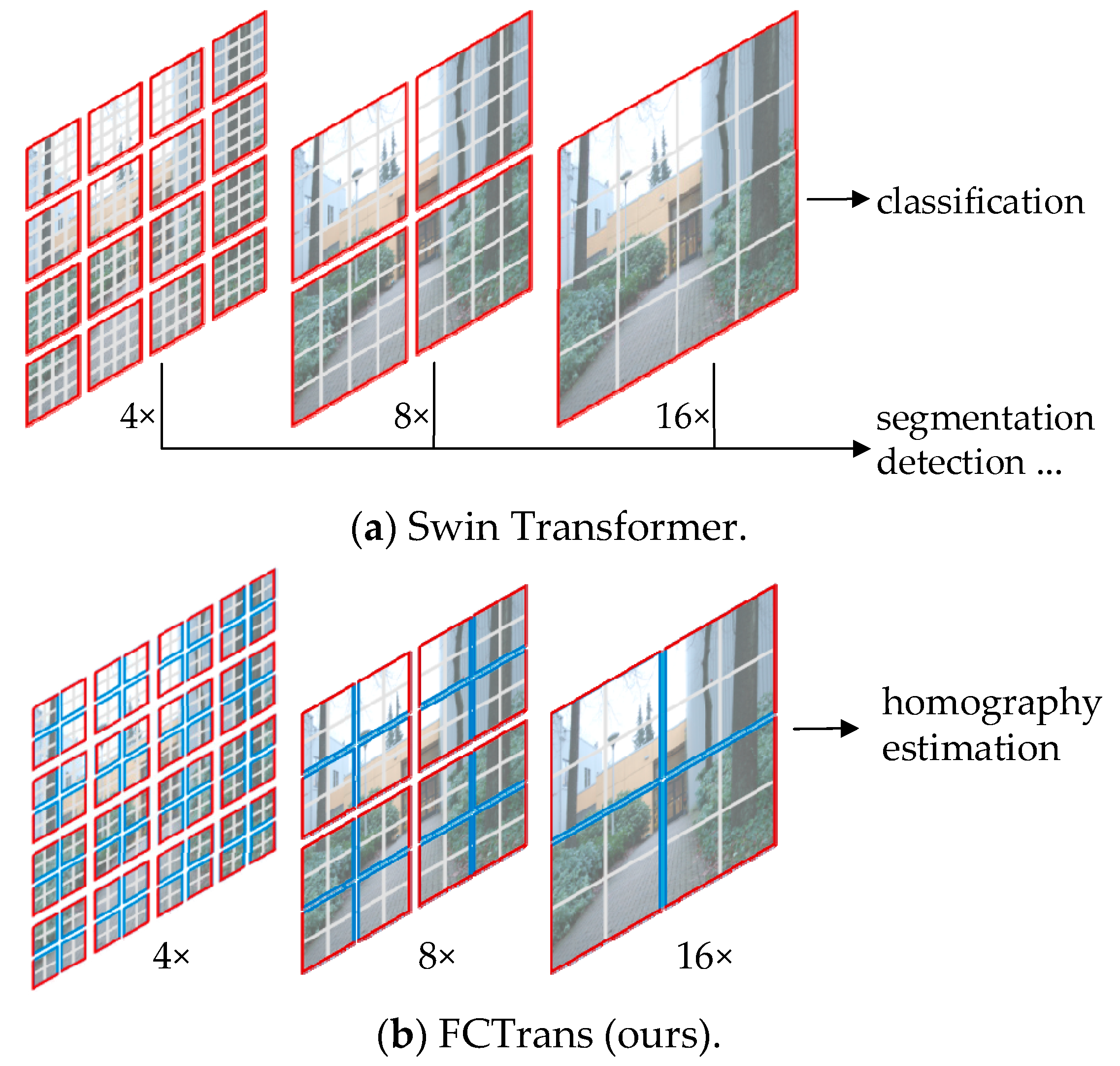
Figure 1. (a) The Swin Transformer computes attention in the unit of pixels (shown in gray) in each local window (shown in red). (b) The proposed FCTrans computes attention in the unit of the feature patch (shown in blue), 2 × 2 in size, in each local window (shown in red), thus efficiently capturing high-level semantic features and adapting to differences between multi-source images.
Remotesensing 15 03535 g001
Figure 2. Overall architecture of the deep homography estimation network. The network architecture consists of four modules: two shallow feature extraction networks (an infrared shallow feature extraction network, f r ( · ) , and a visible shallow feature extraction network f v ( · ) ), an FCTrans generator, and a discriminator. Two consecutive blocks of FCTans used to output different feature maps ( F v l + 1 , F r l + 1 , and F c l + 1 ) are shown at the top of the figure. W-CIA and SW-CIA are cross-image attention modules with regular and shifted window configurations, respectively.
Remotesensing 15 03535 g002
Figure 3. The overall architecture of the FCTans. In the l -th FCTrans block, we consider F v l as the query feature map (source feature map), F c l as the key/value feature map (projected target feature map), and F r l as the reference feature map (unprojected target feature map).
Remotesensing 15 03535 g003
Figure 4. An illustration of the feature patch in the proposed FCTrans architecture. In layer l (illustrated on the left), we employ a regular window partitioning scheme to partition the image into multiple windows and then further evenly partition them into feature patches inside each window. In the next layer, l + 1 (illustrated on the right), we apply a shifted window partitioning scheme to generate new windows and similarly evenly partition them into feature patches inside these new windows.
Remotesensing 15 03535 g004
Figure 5. Network architecture of cross-image attention. Cross-image attention identifies the correlation between a feature patch in the source feature map and all feature patches in the target feature map within a window. The dimensionality of each feature patch is 2 × 2 .
Remotesensing 15 03535 g005
Figure 6. Some samples from the real-world dataset. Row 1 shows the visible images; row 2 shows the infrared images.
Remotesensing 15 03535 g006
Figure 7. Comparison with the eight traditional feature-based methods in the two examples, shown in (1), (3) and (2), (4). The “Nan” in (2) and (3) indicates that the algorithm failed and the warped image could not be obtained. From left to right: (a) visible image; (b) infrared image; (c) ground-truth infrared image; (d) SIFT [20] + RANSAC [36]; (e) SIFT [20] + MAGSAC++ [38]; (f) ORB [22] + RANSAC [36]; (g) ORB [22] + MAGSAC++ [38]; (h) BRISAK [23] + RANSAC [36]; (i) BRISAK [23] + MAGSAC++ [38]; (j) AKAZE [24] + RANSAC [36]; (k) AKAZE [24] + MAGSA C++ [25]; and (l) the proposed algorithm. We mixed the blue and green channels of the warped infrared image with the red channel of the ground-truth infrared image to obtain the above visualization and the remaining visualizations in this paper using this method. The unaligned pixels are presented as yellow, blue, red, or green ghosts.
Remotesensing 15 03535 g007
Figure 8. Comparison with the three deep learning-based methods in the two examples, as shown in (1) and (2). From left to right: (a) visible image; (b) infrared image; (c) ground-truth infrared image; (d) CADHN [43]; (e) DADHN [46]; (f) HomoMGAN [47]; and (g) the proposed algorithm. Error-prone regions are highlighted using red and yellow boxes, and the corresponding regions are zoomed in.
Remotesensing 15 03535 g008
Figure 9. Ablation studies on the FCL. From left to right: (a) visualization of attention weights on w/o. FCL; (b) the channel mixing result w/o. FCL with an average corner error of 5.17; (c) visualization of attention weights on the proposed algorithm; and (d) the channel mixing result for the proposed algorithm with an average corner error of 4.71. In particular, we normalized the attention weights of the first window in the last FCTrans block to range from 0 to 255 for visualization.
Remotesensing 15 03535 g009
Table 1. The experiment’s environmental parameters.
ParameterExperimental Environment
Operating SystemWindows 10
GPUNVIDIA GeForce RTX 3090
Memory64 GB
Python3.6.13
Deep Learning FrameworkPytorch 1.10.0/CUDA 11.3
Table 2. Network parameters of the proposed method.
ParameterValue
Image Size 150 × 150
Image Patch Size 128 × 128
Initial Learning Rate0.0001
OptimizerAdam
Weight Decay0.0001
Learning Rate Decay Factor0.8
Batch Size32
Epoch50
Window Size (M)16
Feature Patch Size2
Channel Number (C)18
Block Numbers{2,2,6}
Table 3. Comparison of corner errors between the proposed algorithm and all other methods on the synthetic benchmark dataset.
(1)MethodEasyModerateHardAverageFailure Rate
(2) I 3 × 3 4.595.716.775.790%
(3)SIFT [20] + RANSAC [36]50.87NanNan50.8793%
(4)SIFT [20] + MAGSAC++ [38]131.72NanNan131.7293%
(5)ORB [22] + RANSAC [36]82.64118.29313.74160.8917%
(6)ORB [22] + MAGSAC++ [38]85.99109.14142.54109.1319%
(7)BRISAK [23] + RANSAC [36]104.06126.8244.01143.224%
(8)BRISAK [23] +MAGSAC++ [38]101.37136.01234.14143.424%
(9)AKAZE [24] + RANSAC [36]99.39230.89Nan159.6643%
(10)AKAZE [24] + MAGSAC++ [38]101.36210.05Nan139.452%
(11)CADHN [43]4.095.216.175.250%
(12)DADHN [46]3.845.016.095.080%
(13)HomoMGAN [47]3.854.996.055.060%
(14)Proposed algorithm3.754.705.944.910%
The black bold number indicates the best result.
Table 4. Comparison of point matching error between the proposed algorithm and all other methods on the real-world dataset.
(1)MethodEasyModerateHardAverageFailure Rate
(2) I 3 × 3 2.363.634.993.79Nan
(3)SIFT [20] + RANSAC [36]135.43NanNan135.4396%
(4)SIFT [20] + MAGSAC++ [38]165.54NanNan165.5496%
(5)ORB [22] + RANSAC [36]40.0563.23159.7076.5722%
(6)ORB [22] + MAGSAC++ [38]61.69109.96496.02158.8727%
(7)BRISAK [23] + RANSAC [36]44.2281.51483.76151.4724%
(8)BRISAK [23] +MAGSAC++ [38]66.09129.58350.06142.7527%
(9)AKAZE [24] + RANSAC [36]71.77170.03Nan83.3366%
(10)AKAZE [24] + MAGSAC++ [38]122.64NanNan122.6471%
(11)CADHN [43]2.073.274.653.460%
(12)DADHN [46]2.103.274.663.470%
(13)HomoMGAN [47]2.003.154.543.360%
(14)Proposed algorithm1.692.553.792.790%
Table 5. Results of the ablation studies. Each row is the result from our method, with specific modifications. For more details, please refer to the text.
(1)ModificationEasyModerateHardAverage
(2)Change to the Swin Transformer backbone4.015.026.085.13
(3)w/o. feature patch3.824.975.995.02
(4)Change to self-attention and w/o. FCL3.964.965.915.03
(5)w/o. FCL3.945.016.065.10
(6)Proposed algorithm3.754.705.944.91
Disclaimer/Publisher’s Note: The statements, opinions and data contained in all publications are solely those of the individual author(s) and contributor(s) and not of MDPI and/or the editor(s). MDPI and/or the editor(s) disclaim responsibility for any injury to people or property resulting from any ideas, methods, instructions or products referred to in the content.