Computing the Radar Cross-Section of Dielectric Targets Using the Gaussian Beam Summation Method

Abstract

Computing the Radar Cross-Section (RCS) of a given object is a topic of major importance for many applications, e.g., target detection and stealth technology. In this context, high-frequency asymptotic methods are widely used. In this article, we derive a Gaussian Beam Summation (GBS) method for both metallic and dielectric targets. The basic idea is to use the GBS method to compute the scattering far fields generated by the equivalent currents flowing on the surfaces. The validity of the proposed method is then investigated in the X-band. To accomplish this, the results obtained using this technique were compared to those obtained using other sufficiently accurate methods such as the ray tracing of FEKO and the ray asymptotic solution. As an example of the method’s accuracy, the GBS method was used to obtain the wave field in a homogeneous medium by fitting the results to a point source. In the same way, the method was used to compute the RCS of dielectric cuboids.

1. Introduction

In this paper, we are interested in computing the Radar Cross-Section (RCS) of an electrically large object. As a matter of fact, modeling the electromagnetic wave scattering from a given object is a topic of major interest for many applications, such as detection (e.g., radar [1,2]), stealth technology validation and optimization [3], or inverse problems (e.g., inverse scattering [4]). This problem becomes quite challenging when the objects are electrically large. Indeed, rigorous methods, such as the Method of Moments (MoM) [5], are limited by their computational performance since the mesh size needs to be at least $\lambda /8$.

Therefore, high-frequency asymptotic techniques, such as ray methods [6] or Physical Optics (PO) [7,8], have been extensively employed in order to find approximate solutions in a limited amount of time while maintaining good accuracy. In general, the latter comes from an asymptotic evaluation of existing Green’s functions for given conditions.

For example, Geometrical Optics (GO) [6,9] is based on the description of the field in terms of optical rays–plane waves–that follow Fermat’s rule and are summed together at a given point to obtain the electric or magnetic field at this point. The latter is limited by the number of rays needed to accurately describe complicated shapes and by caustic phenomena. Another widely used asymptotic method is the PO method [7,8,10]. This technique corresponds to the asymptotic version of the MoM, where only the surface of the object is discretized and the radiation integral is computed over a set of equivalent currents on the surface. This computation is performed by assuming that the incident field is a plane wave and that each facet is locally plane, leading to an easier calculation of the currents. For complex shapes, shade areas need to be determined in order to use PO efficiently; thus, GO is used. Nevertheless, both these methods compute accurate estimates of the field behavior in the specular regions [11]. Additionally, they offer clear physical images that can be used to analyze how electromagnetic waves propagate in real-world contexts.

However, they do not take into account diffraction effects. As a consequence, some improvements have been proposed to overcome this problem such as the Geometrical Theory of Diffraction (GTD) [12,13], the Uniform Theory of Diffraction (UTD) [14,15,16], or the Physical Theory of Diffraction (PTD) [17,18]. They consist of a theoretical extension of GO (or PO) that provides a more comprehensive explanation of the mechanism of high-frequency wave propagation, i.e., diffraction and reflection, in order to correct the field computations outside the specular region. Nevertheless, the caustics problem persists and the computational efficiency decreases since more rays need to be accounted for.

In the 1980s, a new asymptotic method was introduced, where the field was described in terms of Gaussian beams, thereby overcoming the caustic problem [19,20]. Indeed, the Helmholtz equation was reduced to the Parabolic Wave Equation (PWE) [21], and a solution was sought in the form of a Gaussian beam. Since then, the method has been widely used to model electromagnetic wave propagation [22,23,24,25,26] for diverse applications. In particular, in the context of the RCS computation, two main methods have been employed: the Gaussian Beam Summation (GBS) [27,28,29,30] and the Gaussian Beam Launching (GBL) [23,25] techniques. The latter can be compared to the PO method. GBS works in the same way as the GO method, but rays are replaced by Gaussian beams. Indeed, the incident wave is assumed to be a Gaussian beam instead of a plane wave, but the overall principle remains the same.

The above-mentioned methods use conventional techniques to calculate the far scattering field generated by an electric current on a perfectly conducting surface. However, extensions are needed when dealing with dielectric targets and/or when dealing with a target on a dielectric ground (such as the sea). Usually, the scattering field for dielectric targets is generated by electric and magnetic equivalent currents, excited by the reflected electric and magnetic fields, and formulated using the Kirchhoff approximation [31,32] and the Fresnel coefficients.

In this paper, we are interested in extending the GBS approach to the RCS computation when dealing with large dielectric objects. To the best of the author’s knowledge, this extension to the RCS computation has not been dealt with before since the GBS method has only been used to compute the RCS of perfectly metallic objects [27,28,29]. Therefore, we propose to use the Fresnel reflection coefficient [33] in the same way as for the PO method in order to compute the scattered field from a dielectric material. Some numerical tests in the X-band are conducted to validate the proposed method and compare it with the PO method and FEKO. Additionally, the influence of some parameters on the GBS approach’s accuracy is tested.

The remainder of this article is organized as follows. Section 2 comprises three subsections that outline the problem formulation, notations, and step-by-step implementation of the GBS method. Initially, we present the 2D GBS method tailored for metallic scatterers, followed by its extension to incorporate dielectric targets. Furthermore, we detail the formulation of the 3D GBS method, enabling us to analyze scattering phenomena in a 3D space. In Section 3, we conduct a sensitivity analysis of the GBS method, examining its performance under different parameter settings. We then apply the GBS method to compute the RCS of metallic targets and compare our results with those of FEKO and the PO method. Additionally, we employ the GBS method to determine the RCS of a dielectric cuboid and offer insightful discussions on its characteristics. Lastly, Section 4 concludes this paper, discusses the method, and provides some perspectives for future works.

2. Materials and Methods

In this section, we provide an overview of the problem formulation and introduce the notations used throughout the article to ensure clarity and consistency. We then delve into the GBS method, which is presented in three distinct parts. First, we explore the implementation and intricacies of the GBS method when applied to metallic scatterers in a two-dimensional setting. Next, we discuss the modifications and considerations necessary to accurately compute the RCS of dielectric targets using the GBS method. Finally, we present the formulation of the three-dimensional GBS method, enabling the modeling and analysis of complex radar targets.

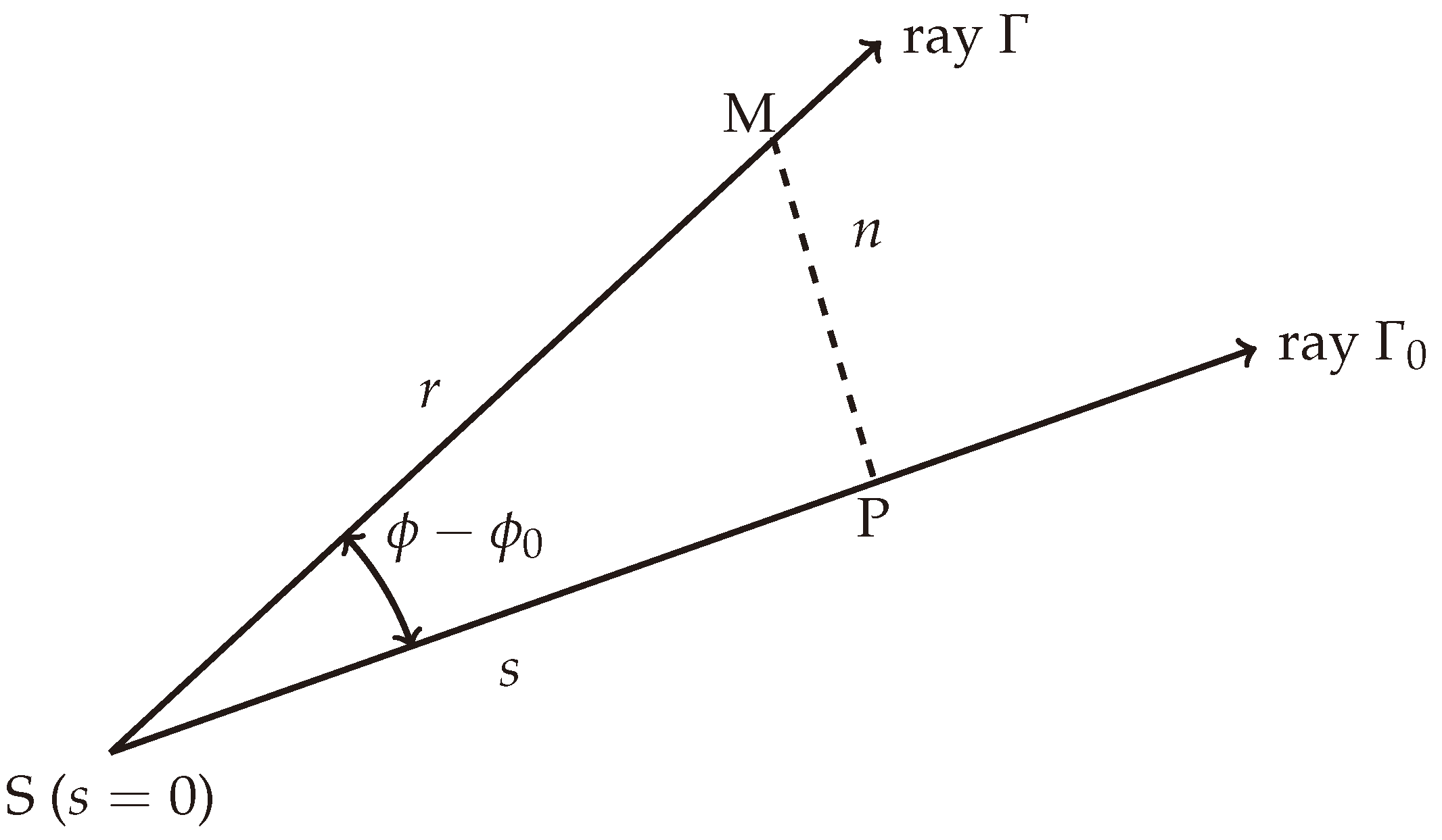
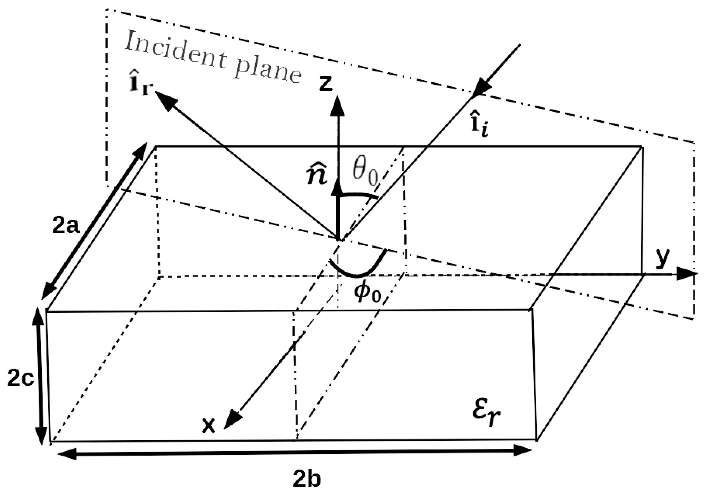
2.1. Formulation of the Problem and Notations

Let us begin by introducing the notations that are used in this article. The vectors and matrices are denoted in bold such as $\mathit{V}$ and $\mathbf{M}$. A unit vector is denoted with a hat such as $\widehat{\mathit{v}}$. The imaginary unit is denoted by j, and an $exp\left(j\omega t\right)$ time dependence is assumed in this paper, with $\omega$ being the angular frequency. The frequency is denoted by f, and k denotes the wave number. The computations are performed in a non-empty domain $\mathsf{\Omega }$, corresponding to free space. The usual notations $\mathit{E}$ and $\mathit{H}$ are used for the electric and magnetic fields, whereas ${\mathit{J}}_e$ and ${\mathit{J}}_m$ denote the electric and magnetic surface current densities, respectively.

As mentioned in the introduction, we are interested in the computation of the RCS of a dielectric or metallic target, i.e., computing the scattered field when an incident field hits the object $\mathcal{O}$. The latter is assumed to be in the center of the domain. In this context, we are interested in obtaining the electrical field $\mathit{E}$ to compute:

$$\sigma =\underset{r\to \infty }{lim}4\pi r^2\frac{\parallel {\mathit{E}}^{\mathrm{s}}{\parallel }^2}{\parallel {\mathit{E}}^{\mathrm{i}}{\parallel }^2},$$

(1)

where $\sigma$ denotes the RCS, ${\mathit{E}}^s$ and ${\mathit{E}}^i$ denote the scattered and incident fields, respectively, and r denotes the distance from the object. A schematic representation of the problem is given in Figure 1, where the target is plotted in red. The target is a dielectric object of relative permittivity ${\epsilon }_r\in \mathbb{C}$, which is assumed to be constant in all $\mathcal{O}$.

In this paper, we want to compute ${\mathit{E}}^{\mathrm{s}}$ (and thus $\sigma$) at a given distance from the object r, where $r\gg \lambda$, with an object electrically large, i.e., its dimension D is such that $D\gg \lambda$. Thus, an asymptotic method is developed here to efficiently compute the RCS under these conditions. Indeed, with a rigorous method such as the MoM, the computations would be time-consuming and have a large memory footprint. The computations are performed in both 2D and 3D.

2.2. The Gaussian Beam Summation Method

In this section, the complete asymptotic computational scheme is developed. First, we recall the usual 2D GBS method when only a metallic object is accounted for. Second, the method is extended to account for dielectric targets. Finally, the 3D formulation for the GBS method is explained.

2.2.1. The 2D GBS Method for a 2D Metallic Scatterer

For better readability and understandability, the GBS method is recalled in 2D. The usual Cartesian coordinates $(x,z)$ are used. In this context, the field can be decomposed into transverse electric (TE) and transverse magnetic (TM) components with respect to the z-axis. In both cases, either the field $\mathit{E}$ or $\mathit{H}$ has only one non-zero component, i.e., $E_y$ and $H_y$ here. Therefore, we can study the scalar Helmholtz equation defined by:

$${\nabla }^2\mathsf{\Psi }(x,z,\omega )+k{\left(\omega \right)}^2\mathsf{\Psi }(x,z,\omega )=0,$$

(2)

where $\mathsf{\Psi }=E_y$ or $\mathsf{\Psi }=H_y$, and $\omega =2\pi f$. The latter can be rewritten [19] as follows:

$${\nabla }^{2}u\left(x,z,w\right)+\frac{{\omega }^2}{c_0^2}u\left(x,z,w\right)=0,$$

(3)

where $c_0$ is the velocity of light in free space at a given point, and u is the reduced field. Let $\mathsf{\Psi }$ and u be elements of the set $\mathsf{\Omega }$, where $\mathsf{\Omega }$ corresponds to free space.

Then, a new coordinate system $(s,n)$, i.e., the ray-centered coordinate system, is introduced to solve Equation (3). The latter is pictured in Figure 2. The idea of the GBS method is to search the solution u in terms of Gaussian beams [19,20]. One can think of Gaussian beams as a new basis for our field. Note that s corresponds to the path length along the ray, whereas n corresponds to the path length perpendicular to the ray. Also, in $(s,n)$, we denote $v\left(s\right)=c_0$ as the velocity along the ray. The latter simplifies the relations given in [19].

In these new coordinates, one can show that the reduced field u can be obtained as follows [19,20]:

$$u(s,n,\omega )={\left({\displaystyle \frac{c_0}{Q\left(s\right)}}\right)}^{1/2}exp\left(j\omega \tau \left(s\right)+\frac{j\omega }{2}\frac{P\left(s\right)}{Q\left(s\right)}{n}^2\right),$$

(4)

where the ray-centered coordinate system around ${\mathsf{\Gamma }}_0$ is provided. The central ray, denoted as ${\mathsf{\Gamma }}_0$, connects the computation point (where calculations or measurements are made) to the source (the origin or starting point of the rays). In this new system, any other ray such as $\mathsf{\Gamma }$ can be computed. In Equation (4), $\tau \left(s\right)$ is the travel time along the ray path, and Q and P are solutions of the following differential equation system:

$$\begin{array}{ccccc}\hfill {\displaystyle \frac{dQ\left(s\right)}{ds}}& =& c_{0}P\left(s\right)\hfill & \mathrm{with}& Q\left(s_0\right)={\displaystyle \frac{-j\omega L_{\mathrm{M}}^2}{2c_0}}\hfill \\ \hfill {\displaystyle \frac{dP\left(s\right)}{ds}}& =& 0\hfill & \mathrm{with}& P\left(s_0\right)={\displaystyle \frac{1}{c_0}}\hfill \end{array}$$

(5)

In the latter, $P_0$ and $Q_0$ correspond to the Hill’s initial conditions [34], and $L_{\mathrm{M}}$ corresponds to the beam width at a given angular frequency $\omega$. Both the initial values of $P\left(s\right)$ and $Q\left(s\right)$ determine the width and wavefront curvature of the Gaussian beams. A more thorough discussion on the choice of the parameter $L_{\mathrm{M}}$ is given in [19]. Note that the form of u in Equation (4) comes from the narrow-angle paraxial wave equation given in [19,20], assuming a Gaussian beam as the solution. Thus, the results are accurate in a paraxial cone of around 10° around the ray. Also, u corresponds to a given ray $\mathsf{\Gamma }$. Additionally, this solution is well behaved when:

$$\mathrm{Im}\left({\displaystyle \frac{P\left(s\right)}{Q\left(s\right)}}\right)>0\mathrm{and}\left|Q\left(s\right)\right|\ne 0\forall s.$$

(6)

The optimal choice of the beam width $L_{\mathrm{M}}$ [19,20] depends on the frequency and distance along the ray from the initial point and is given by:

$$L_{\mathrm{M}}={\left[\frac{2c_0}{\omega }(s-s_0)\right]}^{1/2},$$

(7)

where $s-s_0$ corresponds to the distance to the center of the object $\mathcal{O}$. In the following, we assume that the object is at the center of the domain leading to $s-s_0=s.$

To compute the field at a given point M, we need to sum all the contributions of the different Gaussian beams arriving at this point, as with the GO or PO methods. Using the linearity of the wave in Equation (3), an approximate solution is given by the following expression:

$$u\left(M\right)={\int }_0^{2\pi }\mathsf{\Phi }\left(\varphi \right)u_{\varphi }(r,\varphi ,{\varphi }_0)d\varphi ,$$

(8)

where ${\varphi }_0$ is the direction of the central ray toward M, r is the distance of M from the object, $u_{\varphi }$ corresponds to one contribution, and $\mathsf{\Phi }$ corresponds to a weight function for each Gaussian beam. If the latter was known, then the integral could be directly computed. Therefore, a procedure to approximate it is described later. Furthermore, to compute the integral, we need to express each $u_{\varphi }$ in the $(r,\varphi )$ coordinate system.

Therefore, we begin by expressing $u_{\varphi }$ in the polar coordinate system $(r,\varphi )$. To do so, the differential Equation (5) needs to be solved leading to:

$$\begin{array}{cc}\hfill P\left(s\right)& =c_0^{-1}\hfill \\ \hfill Q\left(s\right)& =(s-s_0)+Q_0\hfill \end{array}$$

(9)

Then, we express $\tau$, s, and n in the $(r,\varphi )$ coordinate system as:

$$\begin{array}{cc}\hfill \tau (\varphi ,{\varphi }_0)& =c_0^{-1}rcos(\varphi -{\varphi }_0)\hfill \\ \hfill s(\varphi ,{\varphi }_0)-s_0& =rcos(\varphi -{\varphi }_0)\hfill \\ \hfill n(\varphi ,{\varphi }_0)& =rsin(\varphi -{\varphi }_0)\hfill \end{array}$$

(10)

Finally, we obtain the following expression for $u_{\varphi }$:

$$\begin{array}{c}{u}_{\varphi }(r,\varphi ,{\varphi }_0)={\left({\displaystyle \frac{c_0}{Q_0+rcos(\varphi -{\varphi }_0)}}\right)}^{1/2}\hfill \\ exp\left(-\omega \left[-{\displaystyle \frac{j}{c_0}}rcos(\varphi -{\varphi }_0)-{\displaystyle \frac{j}{2c_0}}{\displaystyle \frac{r^2{sin}^2(\varphi -{\varphi }_0)}{Q_0+rcos(\varphi -{\varphi }_0)}}\right]\right),\hfill \end{array}$$

(11)

where ${\varphi }_0$ corresponds to the take-off angle of the beam, and r is the distance from the target.

Next, the function $\mathsf{\Phi }$ is computed using the stationary phase theorem [35] as follows. Indeed, for a line source, when $\omega \to \infty$, Equation (8) must correspond to the exact solution of the wave equation, which is:

$$u_{\mathrm{ex}}\left(M\right)=-\frac{1}{4}{\left(\frac{2c_0}{\pi \omega r}\right)}^{1/2}exp\left(j\frac{\omega r}{c_0}+j\frac{\pi }{4}\right).$$

(12)

Therefore, the expression of $\mathsf{\Phi }$ is computed using the stationary phase theorem for $u\left(M\right)$ and $u_{\mathrm{ex}}\left(M\right)$ to coincide. First, assuming a given r and ${\varphi }_0$, the following two functions are introduced:

$$\begin{array}{cc}\hfill F\left(\varphi \right)& ={\left({\displaystyle \frac{c_0}{Q_0+rcos(\varphi -{\varphi }_0)}}\right)}^{1/2}\hfill \\ \hfill f\left(\varphi \right)& =-{\displaystyle \frac{j}{c_0}}rcos(\varphi -{\varphi }_0)-{\displaystyle \frac{j}{2c_0}}{\displaystyle \frac{r^2{sin}^2(\varphi -{\varphi }_0)}{Q_0+rcos(\varphi -{\varphi }_0)}}.\hfill \end{array}$$

(13)

Second, by deriving the function $f\left(\varphi \right)$, the saddle point is obtained for $\varphi ={\varphi }_0$. Then, the second derivative of f is computed at $\varphi ={\varphi }_0$, leading to:

$${\left[\frac{d^{2}f\left(\varphi \right)}{d{\varphi }^2}\right]}_{\varphi ={\varphi }_0}={\displaystyle \frac{j{Q}_{0}r}{c_0(Q_0+r)}}.$$

(14)

The integral (8) is now approximated—steepest descent—as:

$$u\left(M\right)=\mathsf{\Phi }\left({\varphi }_0\right)c_0{\left({\displaystyle \frac{2\pi }{Q_0\omega r}}\right)}^{(1/2)}exp\left(j{\displaystyle \frac{\omega r}{c_0}}-j{\displaystyle \frac{\pi }{4}}\right).$$

(15)

Finally, by equalizing (15) and (12), we obtain:

$$\mathsf{\Phi }\left({\varphi }_0\right)=-{\displaystyle \frac{j}{4\pi }}{\left({\displaystyle \frac{Q_0}{c_0}}\right)}^{1/2}.$$

(16)

Since $Q_0$ does not depend on $\mathsf{\Phi }$, we can conclude [36] that $\mathsf{\Phi }\left(\varphi \right)$ is a complex-valued constant and equals $\mathsf{\Phi }\left({\varphi }_0\right)$ given by Equation (16).

The integral (8) can now be computed for any given ${\varphi }_0$ and r. For numerical reasons, the integral is discretized and computed as follows:

$$u\left(M\right)=\sum _{k=1}^N{\mathsf{\Phi }}_k{u}_{\varphi ,k}\mathsf{\Delta }\varphi ,$$

(17)

where $\mathsf{\Delta }\varphi$ is the angle step. Different discretizations can be performed such as a simple trapezoidal one or a more advanced one like the Simpson one. Hence, for a given metallic target $\mathcal{O}$, the GBS method allows us to compute its RCS. In the following section, the method is extended to account for dielectric targets.

2.2.2. Extension of the GBS Method for Dielectric Targets

In this section, the GBS method is formulated to account for a dielectric object. As mentioned in Section 2.1, $\mathcal{O}$ is assumed to be a dielectric material with a constant ${\epsilon }_r$ in the coating. As with the PO method, we assume locally plane facets, each of them can be pictured as a plane surface, as plotted in Figure 3. The goal here is to derive an extension of the GBS for dielectric materials, similar to the approach used for the PO method [33].

Here, we add the notations ${\mathit{E}}^t$ and ${\mathit{E}}^r$ for the transmitted and reflected fields due to ${\mathit{E}}_i$ striking the dielectric coating, and $\widehat{\mathit{n}}$ for the exterior normal. The computations are performed for a TE-polarized electromagnetic wave, but the calculations remain the same for the TM case. Additionally, the size of the dielectric coating is $2b\times 2c$ along the horizontal and vertical dimensions. The angle of incidence from ${\mathit{E}}^i$ on the object is denoted as ${\theta }_0$.

On the surface of the dielectric object, the following relation needs to be verified:

$$u^i=u^r+u^t.$$

(18)

Assuming that the three are Gaussian beams, we can rewrite them as follows:

$$\begin{array}{cc}\hfill u^i& =\mathsf{\Phi }{\left(\varphi \right)}^{i}exp\left(\omega f^i\left(\varphi \right)\right)\hfill \\ \hfill u^s& =\mathsf{\Phi }{\left(\varphi \right)}^{s}exp\left(\omega f^s\left(\varphi \right)\right)\hfill \\ \hfill u^r& =\mathsf{\Phi }{\left(\varphi \right)}^{r}exp\left(\omega f^r\left(\varphi \right)\right)\hfill \end{array}$$

(19)

Since (18) must be verified for $\omega \to \infty$, we have:

$$f^i\left(\varphi \right)=f^r\left(\varphi \right)=f^t\left(\varphi \right),$$

(20)

as shown in [22]. Therefore, only the weighting function $\mathsf{\Phi }$ must be calculated again here. To do so, as with the PO extension for dielectric objects [33], we use the Fresnel coefficient. Note that this is equivalent to what is proposed for propagation applications with Gaussian frames in [24].

To obtain the appropriate $\mathsf{\Phi }$, as with a PEC, one solution is to calculate it by comparison with another asymptotic approach or analytic solution. Following this idea, let us assume that ${\mathit{E}}^i$ is a plane wave striking the dielectric coating of depth $2c$. Thus, both the electric and magnetic fields are written as follows:

$$\begin{array}{cc}\hfill {\mathit{E}}^i& =E_0{\widehat{\mathit{i}}}_{\mathrm{i}}exp\left(jk{\widehat{\mathit{k}}}_i·{\mathit{r}}^{\prime }\right)\hfill \\ \hfill {\mathit{H}}^i& ={\displaystyle \frac{1}{{\zeta }_0}}{\widehat{\mathit{k}}}_i\times {\mathit{E}}^i,\hfill \end{array}$$

(21)

where $E_0$ is the wave amplitude, ${\widehat{\mathit{i}}}_{\mathrm{i}}$ is the unit polarization vector, ${\widehat{\mathit{k}}}_i$ is the unit wave vector, ${\mathit{r}}^{\prime }$ is the position vector, and ${\zeta }_0$ is the free-space impedance. Then, the reflected wave from the top surface of the target can be expressed using the reflection coefficient as:

$$\begin{array}{cc}\hfill {\mathit{E}}^r& =\mathsf{\Gamma }\left({\theta }_0\right)E_0{\widehat{\mathit{i}}}_{\mathrm{r}}exp\left[-jk\left({\widehat{\mathit{k}}}_{\mathrm{r}}·{\mathit{r}}^{\prime }+2c_{0}cos{\theta }_0\right)\right]\hfill \\ \hfill {\mathit{H}}^r& ={\displaystyle \frac{1}{{\zeta }_0}}{\widehat{\mathit{k}}}_r\times {\mathit{E}}^r,\hfill \end{array}$$

(22)

where $\mathsf{\Gamma }$ corresponds to either the parallel or perpendicular Fresnel reflection coefficient. Thus, the latter can be computed for any given incident plane wave and dielectric material. In this definition, we also have ${\widehat{\mathit{i}}}_{\mathrm{r}}$ and ${\widehat{\mathit{k}}}_{\mathrm{r}}$, which correspond to the unit polarization and wave vector for the reflected field. The latter can be obtained using the Snell–Descartes laws, with:

$${\widehat{\mathit{k}}}_{\mathrm{r}}={\widehat{\mathit{k}}}_{\mathrm{i}}-2\widehat{\mathit{n}}({\widehat{\mathit{k}}}_{\mathrm{i}}·\widehat{\mathit{n}})\mathrm{and}{\widehat{\mathit{i}}}_{\mathrm{r}}={\widehat{\mathit{i}}}_{\mathrm{i}}.$$

(23)

Finally, by using the surface-equivalent principle [37], the scattered field in the exterior region, where r is large, can be computed using the Stratton–Chu (or Trace) formula [31] considering the following equivalent surface electric and magnetic current densities:

$$\begin{array}{cc}\hfill {\mathit{J}}_e& =\widehat{\mathit{n}}\times {\mathit{H}}^r\hfill \\ \hfill {\mathit{J}}_m& =\widehat{\mathit{n}}\times {\mathit{E}}^r.\hfill \end{array}$$

(24)

After radiating the currents to obtain the desired field $u_s$, the function $\mathsf{\Phi }$ is computed using the stationary phase theorem, and the integral (8) is approximated using the steepest descent method, as in Section 2.2.1. The RCS takes the simple form:

$$\sigma ={\sigma }_{\infty }{\left|R_p\right|}^2{\delta }_{pq},$$

(25)

where ${\sigma }_{\infty }$ is the PO/GBS form for the backscatter cross-section of the perfectly conducting target of the same shape, and $R_p$ is the reflection coefficient for an incident wave of polarization $p\in \{vv,hh\}$. The function ${\delta }_{pq}$ is the Kronecker delta. Now that the method has been completely explained in 2D, the extension to 3D is introduced.

2.2.3. Formulation of the 3D GBS Method

According to [38], in 3D, the individual contribution of the beamis given by the equation:

$$u_{\theta }(s,n,\omega )=\left(\frac{ik{Q}_0}{8{\pi }^2}\right)\frac{1}{Q_0+s}exp\left[ik\left(s+\frac{1}{2}\frac{n^2}{Q_0+s}\right)\right]$$

(26)

where $Q_0$ is the arbitrary beam parameter [19,36] subject only to the constraint that $\mathrm{Im}{Q}_0<0$. An exhaustive discussion of the dependence of the Gaussian Beam Summation method on $Q_0$ is provided in [22].

Next, the total field at a given point M corresponds to the sum of all Gaussian beams with different take-off angles $\theta$ arriving at M. This leads to the following integral:

$$u\left(M\right)={\int }_0^{2\pi }{\int }_0^{\pi }\mathsf{\Phi }\left(\theta \right)u_{\theta }(s,n,\omega )sin\left(\theta \right)\mathrm{d}\theta \mathrm{d}\varphi ,$$

(27)

where $u_{\theta }$ is the Gaussian beam defined in Equation (26) with a take-off angle $\theta$, and $\mathsf{\Phi }$ is the weighting function, as in the 2D formulation. This integral can be simplified using the Fubini theorem since, from geometrical considerations, one can show that $u_{\theta }$ does not depend on $\varphi$ [29]. Therefore, the integral is expressed as:

$$u\left(M\right)={\int }_0^{2\pi }\mathrm{d}\varphi {\int }_0^{\pi }\mathsf{\Phi }\left(\theta \right)u_{\theta }(s,n,\omega )sin\left(\theta \right)\mathrm{d}\theta .$$

(28)

To compute $\mathsf{\Phi }$, the same method as in Section 2.2.1 can be used, i.e., matching the integral with a well-known asymptotic result such as the ray theory or PO solution, as shown in [19,36]. Then, the integral is numerically computed as:

$$u\left(M\right)\simeq 2\pi \sum _{k=1}^N\mathsf{\Phi }\left({\theta }_k\right)u_{{\theta }_k}sin\left({\theta }_k\right)\mathsf{\Delta }\theta ,$$

(29)

using a discrete approximation of the integral, such as a Simpson rule [39], where $\mathsf{\Delta }\theta$ is the step along $\theta$.

To account for a dielectric, the same method as the one developed in Section 2.2.2 is used. Indeed, only the weighting function is changed by matching it to the scattered field obtained by radiating the current densities of Equation (24), either analytically or using the PO asymptotic method. An example of a cuboid is given in Section 3 with a numerical test.

3. Numerical Results

In this section, some numerical tests are conducted to show the efficiency of our method. First, a sensitivity analysis of the GBS method is performed, considering different parameters of the Gaussian beam. Second, the method is used to compute the RCS of a PEC target. Finally, the method is applied to a dielectric object.

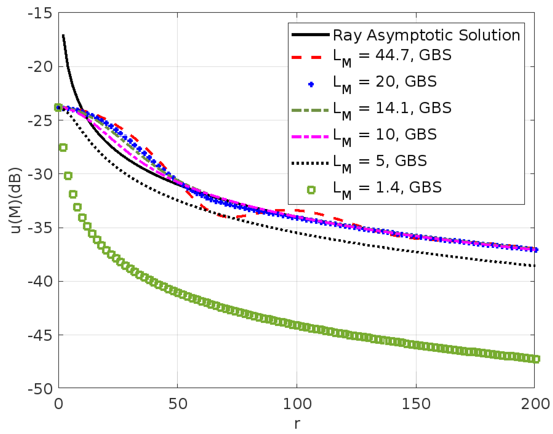
3.1. Sensitivity Analysis of the GBS Method with the Parameters

In this section, we study the impact of some parameters that affect the accuracy of the method:

• The wavelength $\lambda$,
• The distance r between the receiver and the source (the object $\mathcal{O}$),
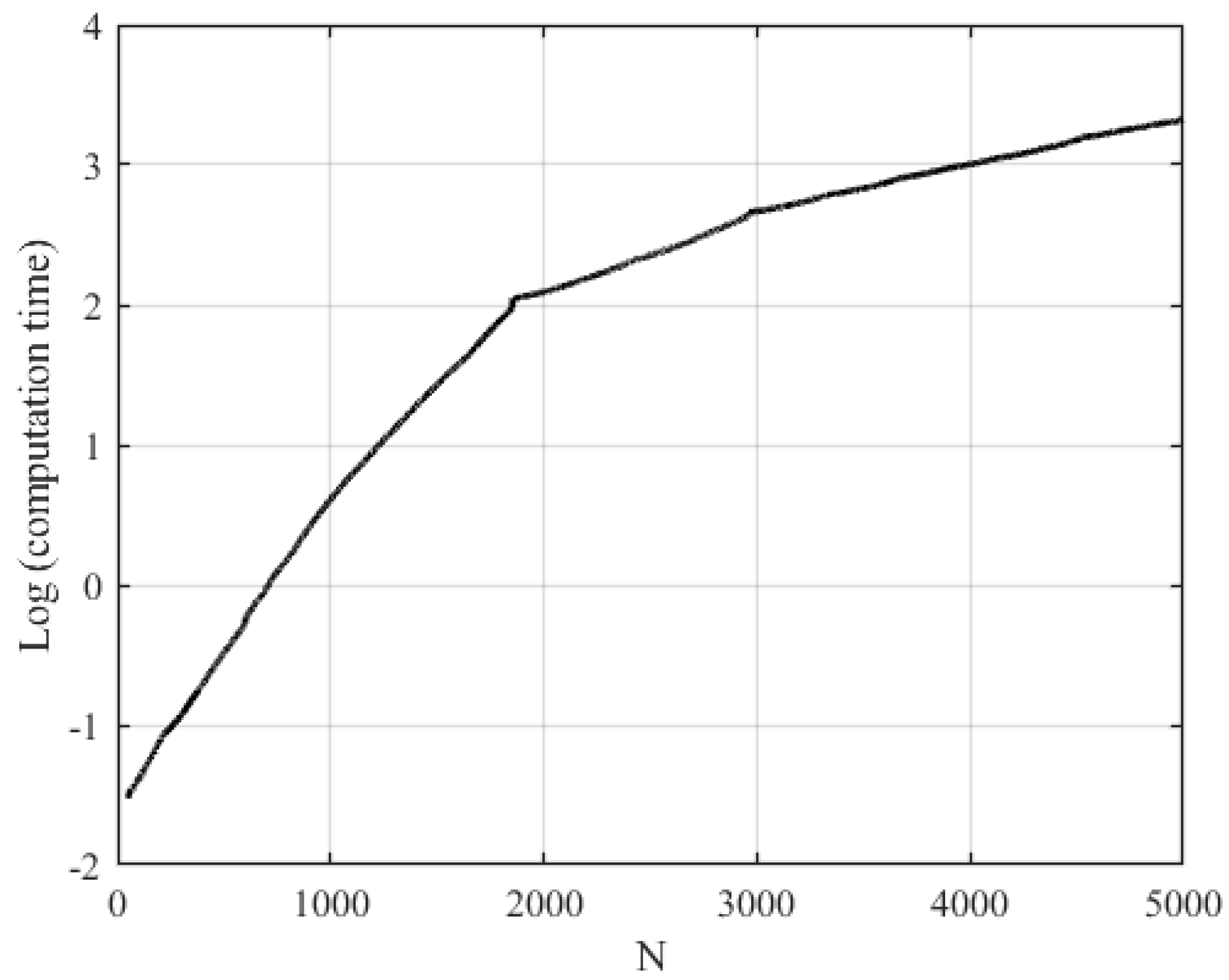
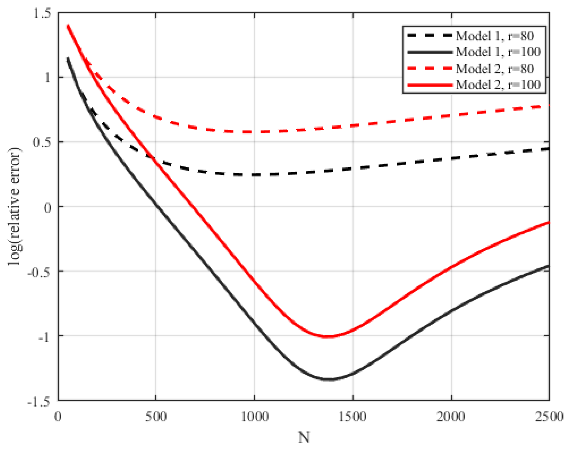
• The number of discreet angles to approximate the integral N,
• The half-beam width $L_{\mathrm{M}}$.

We use the same test as in [36], comparing the results with those provided by the point source [38], to validate the 3D GBS method and its implementation. Note that the field due to the ray asymptotic method is given by:

$$u_{\mathrm{G}}={\displaystyle \frac{exp\left(j\omega r/c_0\right)}{4\pi r}}.$$

(30)

We denote the amplitudes of the GBS method and the ray asymptotic solution as $A_{\mathrm{GBS}}$ and $A_{\mathrm{G}}$, respectively. The phases of the GBS and ray asymptotic methods are denoted as ${\varphi }_{\mathrm{GBS}}$ and ${\varphi }_{\mathrm{G}}$, respectively. Note, that here, the angles are given in radians.

First, we test the effect of the wavelength on the accuracy of the method. The computation parameters are as follows: $r=100$ cm, $\mathsf{\Delta }\theta =0.007$, ${\theta }_{max}=0.6981$, and $N=101$. Here, the angle is measured in both directions from the central ray up to ${\theta }_{max}$. Thus, the wave field is examined in a cone with an angle of $2{\theta }_{max}$. For different $\lambda$, the results in terms of amplitudes and phases are given in

Table 1. Effect of the wavelength $\lambda$ on the GBS results.

$\mathit{\lambda }$	${\mathit{L}}_{\mathbf{M}}$	${\mathit{A}}_{\mathbf{GBS}}$	${\mathit{A}}_{\mathbf{G}}$	${\mathit{\varphi }}_{\mathbf{GBS}}$	${\mathit{\varphi }}_{\mathbf{G}}$
0.62	4.4424	0.00079413	0.00079577	1.8231	1.8242
6.3	14.161	0.00079533	0.00079577	−0.78806	−0.79786
62.8	44.71	0.00074799	0.00079577	−2.2372	−2.5613

. Note that $L_{\mathrm{M}}$ is computed according to (7) for each value of $\lambda$.

From Table 1, one can conclude that the GBS method is in perfect agreement with the ray asymptotic method for different values of $\lambda$. Even for a very large value of $\lambda$, i.e., a lower frequency f, the precision decreases, as expected.

We now test the method using different values of r. The latter increases from 100 cm to 500 cm. The parameters are as follows: $\lambda =6.3$ cm, $\mathsf{\Delta }\theta =0.0087$, $N=101$, and ${\theta }_{max}=0.8727$. The optimal value of $L_{\mathrm{M}}$ is computed for each distance r. The results are provided in

Table 2. The effect of epicenter distance r on the GBS results.

r	${\mathit{L}}_{\mathbf{M}}$	${\mathit{A}}_{\mathbf{GBS}}$	${\mathit{A}}_{\mathbf{G}}$	${\mathit{\varphi }}_{\mathbf{GBS}}$	${\mathit{\varphi }}_{\mathbf{G}}$
100	14.161	0.00079524	0.00079577	−0.78817	−0.79786
200	20.0267	0.0003976	0.00039789	−1.5913	−1.5957
300	24.5277	0.000265	0.00026526	−2.3912	−2.3936
400	28.3221	0.00019869	0.00019894	3.093	3.0917
500	31.6651	0.0001589	0.00015915	2.2943	2.2939

.

As for the test on $\lambda$, we can conclude that the GBS method works well, and the accuracy increases with r, as expected. In the following test, the wavelength $\lambda$, distance r, and step along $\theta$ are fixed to test the effect of the number of discrete angular points N. The test parameters are as follows: $\lambda =6.3$ cm, $r=100$ cm, $\mathsf{\Delta }\theta =0.005$, and $L_{\mathrm{M}}=14.161$. In this case, we have $A_{\mathrm{G}}=0.00079577$ and ${\varphi }_{\mathrm{G}}=-0.79786$. The results in terms of amplitudes and phases are given in

Table 3. The effect of the width of the cone of rays on the GBS results.

N	${\mathit{\varphi }}_{\mathbf{max}}$	${\mathit{A}}_{\mathbf{GBS}}$	${\mathit{\varphi }}_{\mathbf{GBS}}$
121	0.6	0.00079546	−0.78797
101	0.5	0.00079577	−0.78761
81	0.4	0.0008022	−0.8005
61	0.3	0.0008483	−0.72034
41	0.2	0.00069109	−0.4339
21	0.1	0.00025856	−0.13658

.

As expected, with N increasing, i.e., the density of rays, the accuracy of the GBS method increases [19]. Additionally, when $N\ge 101$, the results of the method are in perfect agreement with those obtained using the complex point source.

Finally, we show the effect of the effective half-beam width $L_M$, in particular, when the optimal value is not used. The scenario parameters are $\lambda =6.3$ cm, $\mathsf{\Delta }\theta =0.0075$, ${\theta }_{max}=0.6$, and $N=81$. Note that in this case, the optimal value of $L_{\mathrm{M}}$ would be $14.1$. Additionally, the point source leads to the following values for the amplitude and phase: $A_{\mathrm{G}}=0.00079577$ and ${\varphi }_{\mathrm{G}}=-0.79786$. For the GBS, the results for different $L_M$ are given in

Table 4. The effect of the effective half-width of the beam at the source on the GBS results.

${\mathit{L}}_{\mathbf{M}}$	${\mathit{A}}_{\mathbf{GBS}}$	${\mathit{\varphi }}_{\mathbf{GBS}}$
44.7	0.00077651	−1.0022
20	0.00079607	−0.79492
14.1	0.00079535	−0.78792
10	0.00079238	−0.75847
7.1	0.00076108	−0.66649
5.8	0.00070622	−0.58019

.

This test highlights that the optimal value of $L_{\mathrm{M}}$ is necessary to obtain a good agreement with the expected value.

Figure 4 compares the variation of the electric field obtained by the asymptotic ray theory and the Gaussian Beam Summation method as a function of the distance r. According to this figure, the results are in good agreement for $L_M=10$, $14.1$, and 20 when $r>50$ cm. This confirms the conclusions of Table 2 and Table 4.

In conclusion, this sensitivity analysis shows that, as expected and shown in [19], $L_{\mathrm{M}}$ must be computed using Equation (7), while we need to be further away from the source, i.e., r is large, and at a high frequency, i.e., with a low $\lambda$. Additionally, this shows that the GBS method works well when good parameters are chosen. We can now use it to compute the RCS of different objects $\mathcal{O}$.

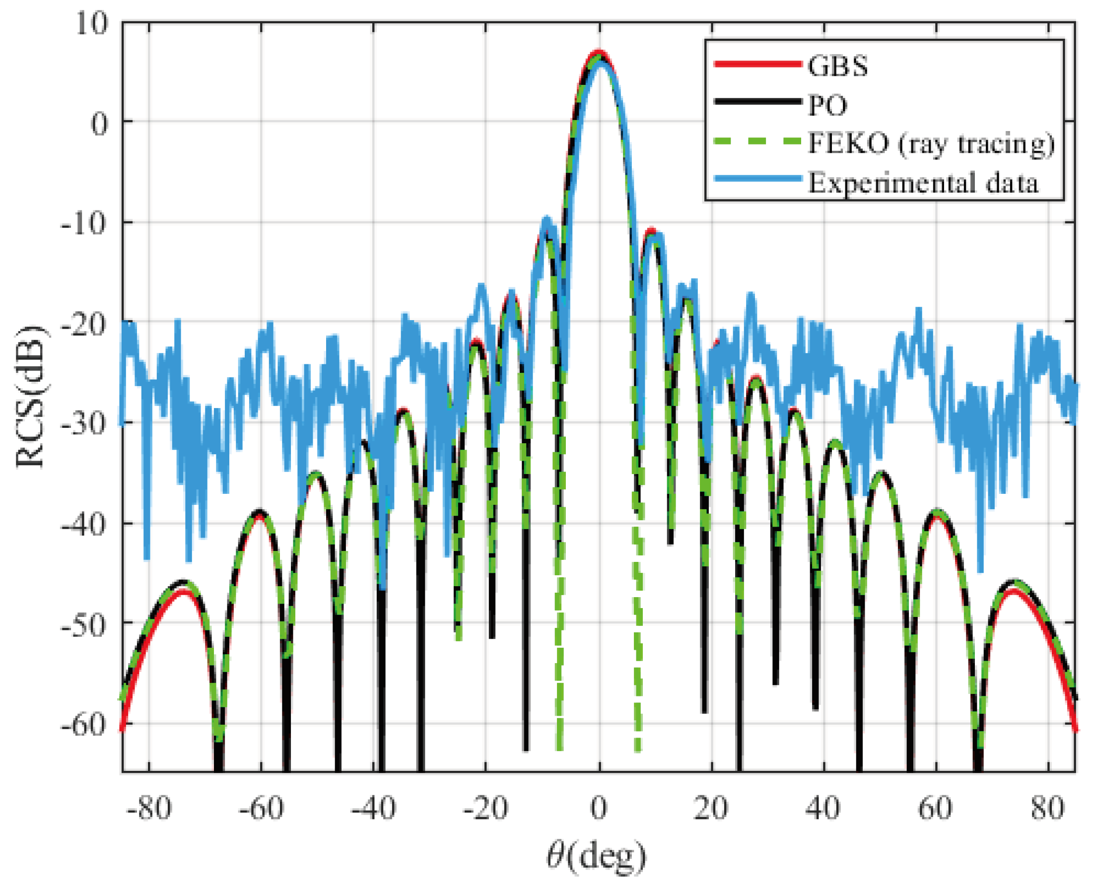
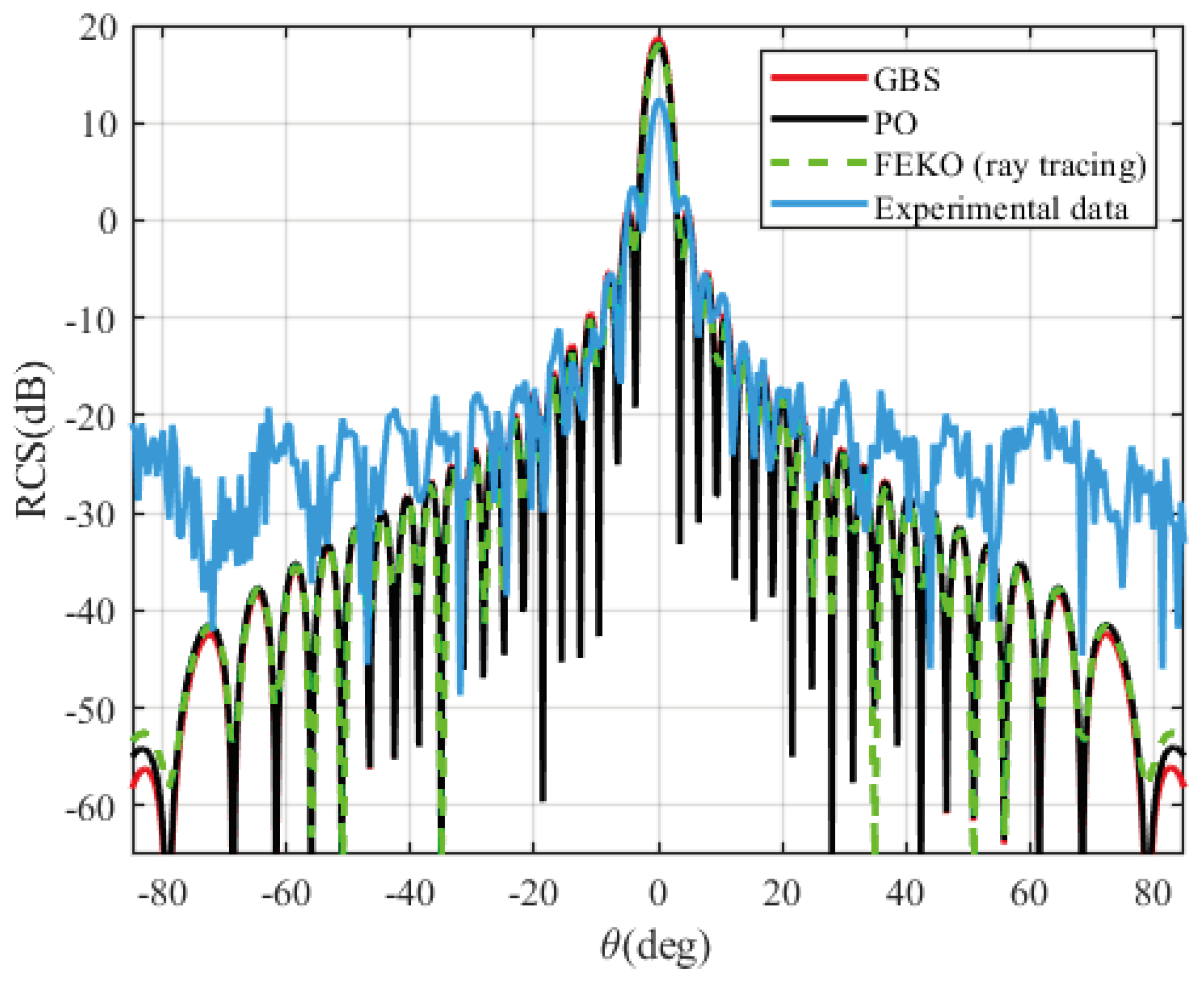
3.2. RCS Computation of Metallic Targets Using the GBS Method

To illustrate the effectiveness of the proposed method, we compute the mono-static RCS of two metallic targets as a function of $\theta$. The investigated targets are a flat circular plate with radius $a=7.5\mathrm{cm}$ ($ka\approx 16$) and a flat circular plate with radius $a=15\mathrm{cm}$ ($ka\approx 31$). The results are shown in Figure 5 and Figure 6. To validate the method, we compare the results with those obtained using the PO method and FEKO software, as well as with experimental data acquired during measurements carried out in an anechoic chamber at ENSTA Bretagne.

The selection of the computation parameters improves the agreement between the GBS results and the analytical results obtained using the PO method and FEKO software, as well as those of the experimental data. The results of the GBS method displayed in Figure 5 and Figure 6 are obtained for $f=10\mathrm{GHz}$, $r=100$, and $N=900$. The parameters $Q_0$ and $L_M$ are defined in Equation (5) and Equation (7), respectively.

Notice the peak at the normal incidence ($\theta =0^{\circ }$) and the decay that rapidly oscillates as a function of $\theta$. With increasing $ka$, the Radar Cross-Section becomes more peaked at the normal incidence and oscillates faster, while the decreasing $ka$ results in a broadened peak and slower oscillations but the shape remains unchanged in general. Regarding Figure 6, the peak of the measurement curve appears lower compared to the other generated curves. This discrepancy in peak amplitude could potentially be attributed to misalignment or deviation from the target’s intended central position during the measurements.

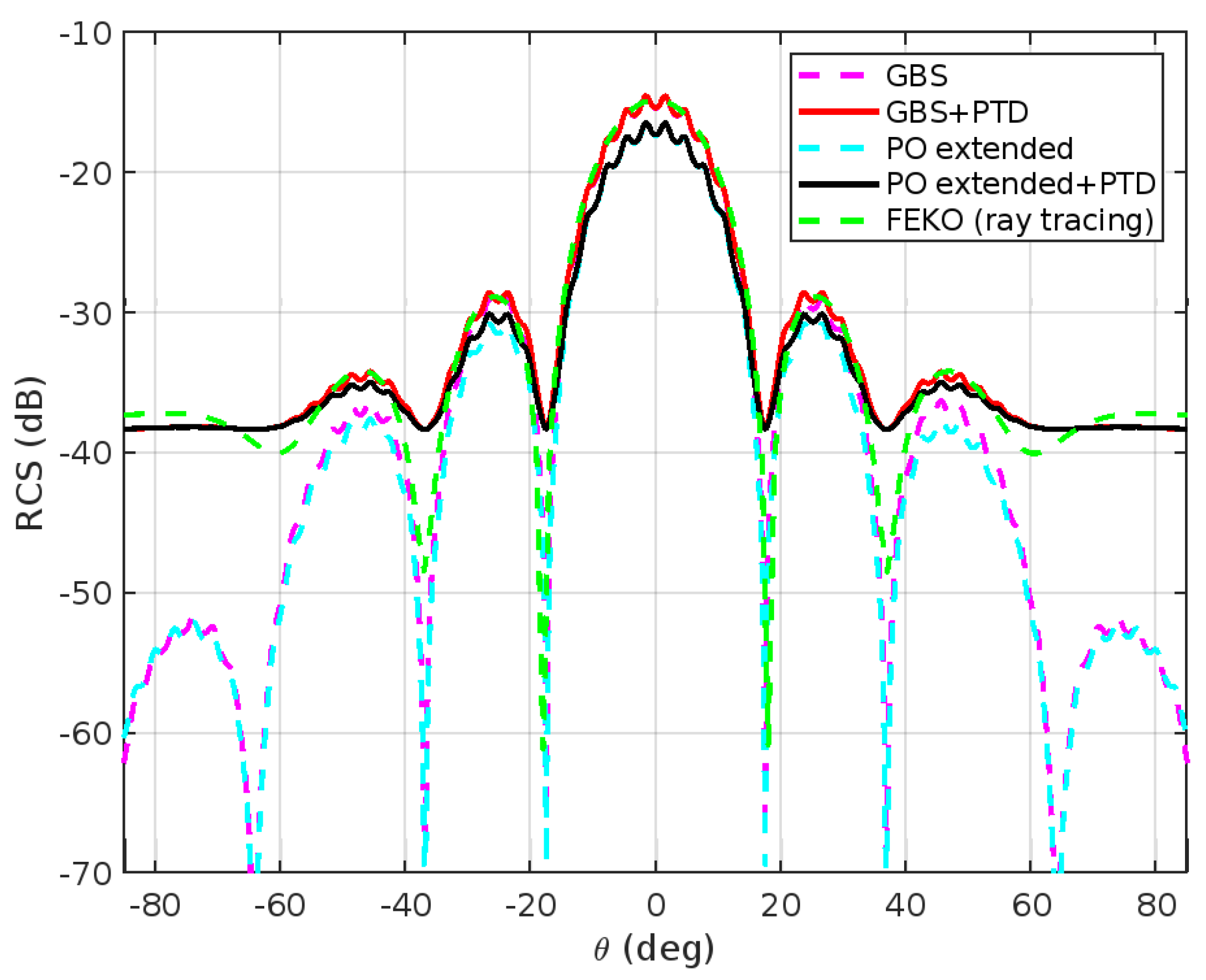
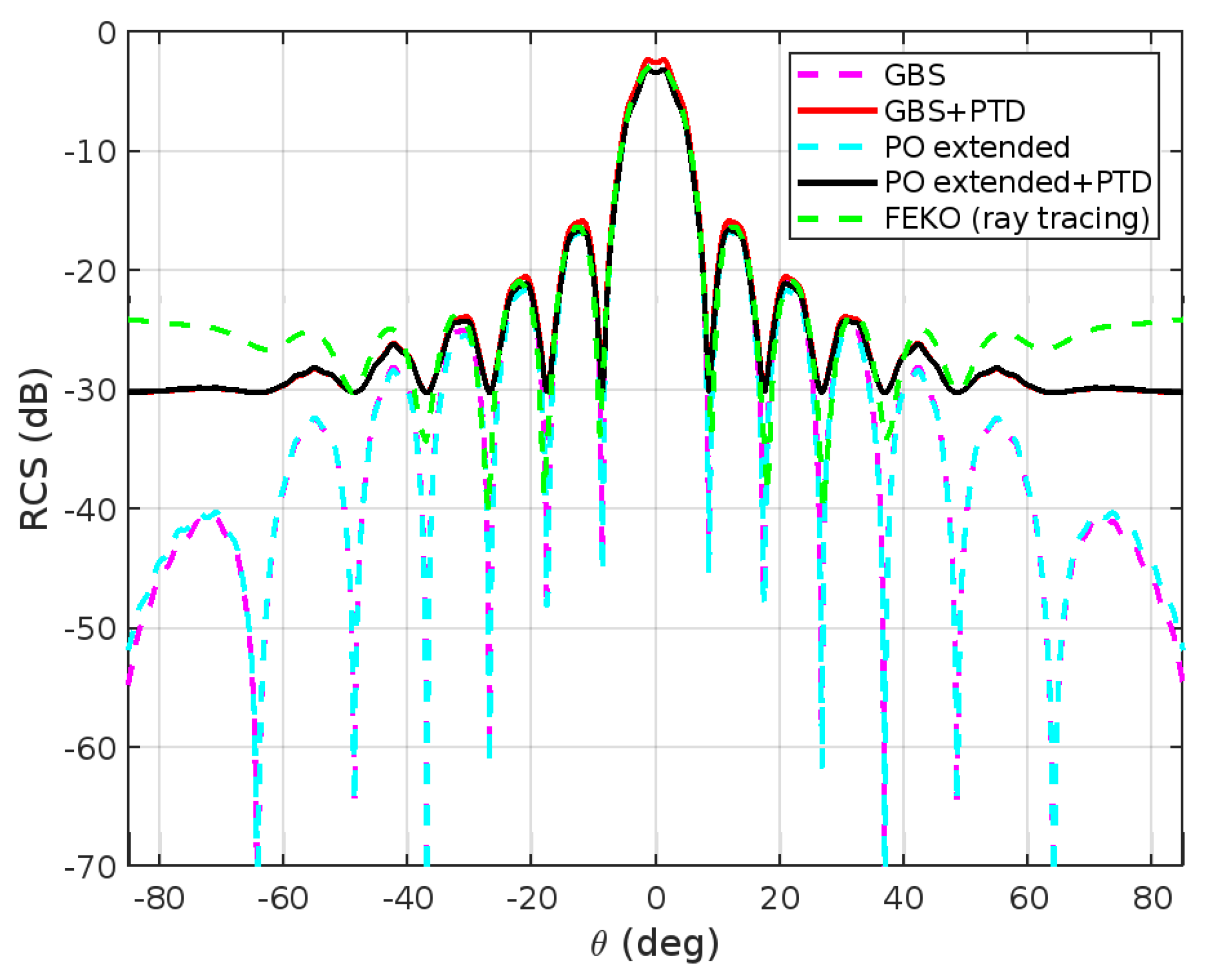
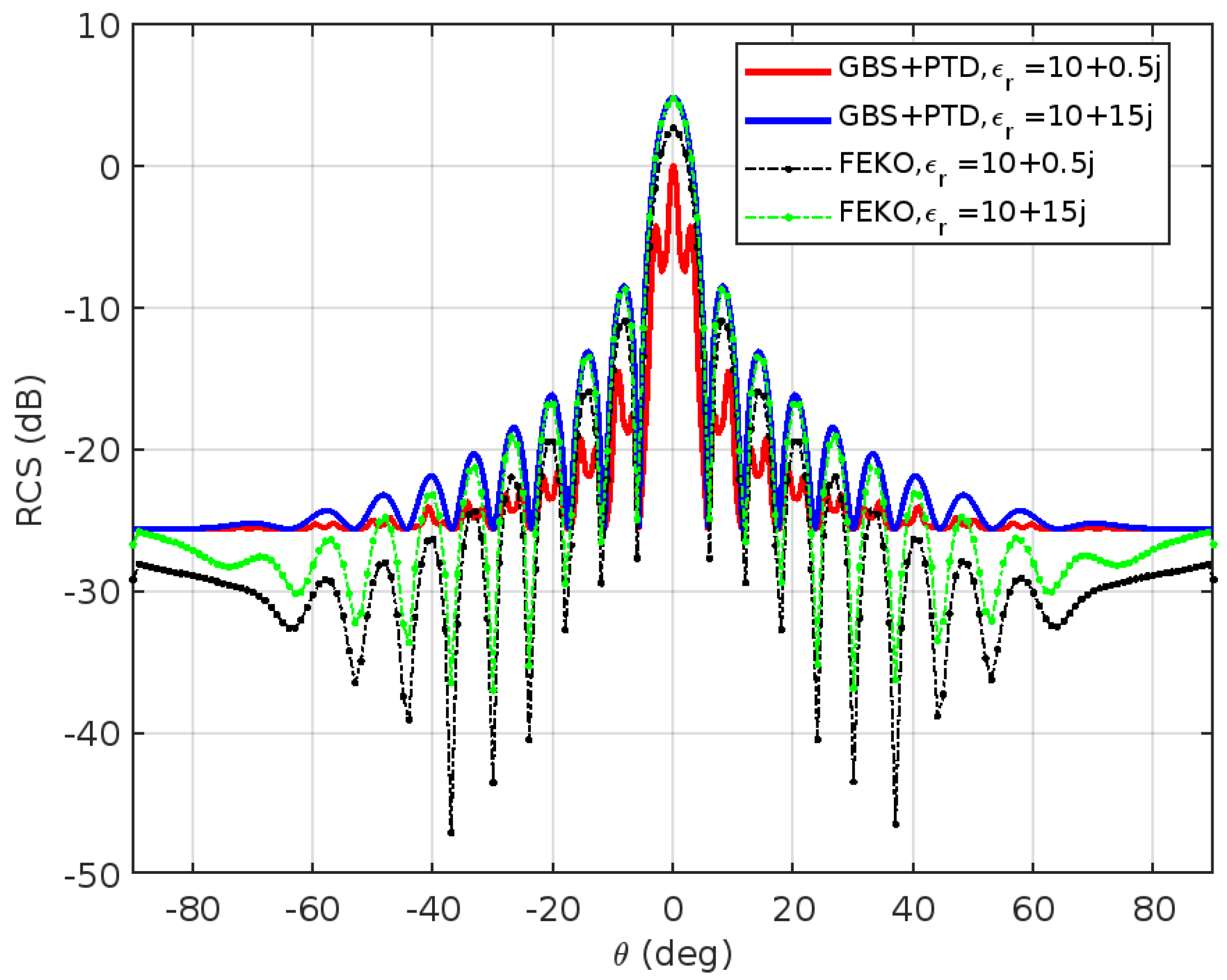
3.3. Numerical Analysis of the GBS Method to Compute the RCS of a Dielectric Cuboid

In this section, the GBS method is used to compute the RCS of a cuboid of dimensions $2a\times 2b\times 2c$, which corresponds to a dielectric material with permittivity ${\epsilon }_r$. The cuboid is pictured in Figure 7. In this case, when a plane wave strikes the cuboid, the electric field can be analytically computed when the observation point is far from the target. Thus, the weighting function $\mathsf{\Phi }$ is computed from this analytical result. Here, we assume a TE-polarized plane wave as the incident field.

First, we use the GBS method to compute the scattered field (or the RCS) of two cuboids with the same dielectric parameters but different sizes. The first one has dimensions of $2a=2b=5$cm and a thickness of $2c=0.5$cm, whereas the second one has dimensions of $2a=2b=10$cm and a thickness of $2c=1$cm. Both are made of the same material with permittivity ${\epsilon }_r=20+2j$. The results of the computations performed using GBS are compared to those obtained using extended Physical Optics [40,41] and the FEKO simulation in Figure 8 and Figure 9. The computational parameters are $f=10$GHz, $r=100$cm, and $N=700$ for Figure 8 and $N=850$ for Figure 9.

In both cases, the proposed method accurately represents the back-scattering phenomena of large rectangular dielectric cuboids illuminated by a TE-polarized plane wave. As can be observed, our approach and the data derived using FEKO are in good agreement in the specular reflection direction and nearby areas, as expected. The extended PO method shows a slightly different result in Figure 8. For greater angles, both the PO and our method currently fail to account for the diffraction caused by the two edges of the rectangular plate.

Nevertheless, the latter could be introduced using the PTD [17], for example. Included in Figure 8 and Figure 9 are the results based on the GBS and PO extended methods, to which we have added the fringe contributions from the side edges thanks to the first-order PTD approximation [42]. It can be seen that the addition of the fringe contributions provides a more accurate description of the RCS close to the grazing angle ($\theta ={90}^{\circ }$). The graph in Figure 8 shows that the RCS estimated using the FEKO simulation and the GBS and PO techniques, each combined with the PTD, all converge to −38 dB at the grazing angle. Examining the plots of the GBS and PO techniques combined with the PTD, respectively, in Figure 9 reveals that the RCS converges to −30 dB at the grazing angle, whereas the FEKO simulation converges to −24 dB.

Second, we test the sensitivity of the method to the dielectric permittivity. Therefore, we study a dielectric cuboid with dimensions of $10\times 10\times 1$cm${}^3$ at $f=10$GHz. Since the GBS method ignores edges near grazing angles, the fringe contributions are calculated using the PTD approximation [42]. Only the real part of ${\epsilon }_r$ is changed for the first test. The results obtained using the GBS method combined with the PTD are compared with those of the commercial FEKO software in Figure 10 for different ${\epsilon }_r$.

As expected, with the real part of ${\epsilon }_r$ increasing, the RCS also increases since the reflection coefficient increases. Additionally, the results obtained using the GBS method and FEKO are in good agreement, particularly in the specular region. Nevertheless, in our method, only the effect of simple diffraction is introduced, yielding slightly different results at the end of the domain of computations.

The following examples are used to test whether the RCS is affected by changing the imaginary part of the dielectric constant. Unless under exceptional circumstances, the behavior of $\sigma$ as a function of $\theta$ remains as illustrated in Figure 8 and Figure 9. Some examples of the Radar Cross-Sections of two different cuboids with different lossy dielectric constants are shown in Figure 11 and Figure 12 and compared to the results obtained using FEKO. $\sigma \left(\theta \right)$ is shown for cuboids with dimensions of $15\times 15$cm${}^2$ and thicknesses of $2c=0.5$cm and $2c=15$cm, respectively, at a frequency $f=10$GHz. Notice the tighter peak at normal incidence and the larger number of oscillations in comparison to Figure 10, which are due to the higher $ka$. The computational parameters for the GBS method are $N=900$ and $r=100$.

The Radar Cross-Section can change drastically when the cuboid thickness becomes an odd multiple of half a wavelength. Figure 11 depicts $\sigma$ in this case. For example, when the thickness is equal to $\lambda /6$ ($2c=0.5$cm) and the relative dielectric constant is ${ϵ}_r=10+0.5j$ (low loss), the waves at the cuboid’s surface add up in phase, and the reflection coefficient is very small. This is especially noticeable at normal incidence, where the peak amplitude is significantly reduced. If the dielectric has higher losses, the amplitude of the field changes as it passes through the cuboid, making this resonance less noticeable.

According to the FEKO results in Figure 12, a symmetric RCS pattern with respect to the angle $\theta =0^{\circ }$ should be observed when the width and thickness of the cuboid are identical. The results of the proposed method are different because it neglects the effect of the other surfaces and the multiple diffractions.

In conclusion, the solution given by the GBS approach applies to arbitrary dielectrics and thicknesses. Nonetheless, simulations for any shape and angle of incidence can be implemented very effectively. However, the proposed method is, by nature, a high-frequency approximation and should, therefore, be applied with caution near the edges or when the minimum dimension of the dielectric target under study is not large compared to the wavelength. Even so, the limitations of the GBS method with respect to the scattered fields near grazing angles are mitigated by taking into account the first-order PTD contributions for the edges.

3.3.1. Trade-Off between Accuracy and Computational Cost

We now proceed to evaluate the efficiency of the method in terms of accuracy and computational time. As a starting point, we plot the algorithm’s execution time as a function of the number of calculation points. This analysis provides valuable insights into the computational efficiency and scalability of the method. Furthermore, we calculate the relative error to assess the accuracy of our method. Our focus is specifically on the specular direction, and we compare it with the corresponding value obtained using FEKO. This analysis provides valuable information regarding the selection of the computational parameters, enabling us to strike a balance between the desired accuracy and the associated computation time and memory requirements.

Figure 13 displays, on a logarithmic scale, the computation time of the GBS algorithm as a function of the number of points N. The resulting curve exhibits a slope of 0.0018. This relatively small slope reinforces the algorithm’s effectiveness, indicating that the increase in computation time remains relatively low as the number of points increases.

To assess the algorithm’s accuracy, we conduct a study involving two models with different sizes. We specifically focus on rectangular targets, one with dimensions of $10\times 10$ cm${}^2$ (model 1) and the other with dimensions of $20\times 20$ cm${}^2$ (model 2), both possessing a permittivity of 3.5. Our evaluation is based on calculating the relative error between the specular direction obtained using the GBS method and the corresponding specular value provided by FEKO.

Our findings in Figure 14 reveal that as the size of the target increases, a greater number of points are necessary to achieve higher levels of accuracy. It is evident that increasing the number of points employed in the calculation generally leads to improved precision. Additionally, it is worth noting that as the value of N increases, it is essential to correspondingly adjust the distance parameter r.

By carefully analyzing the interplay between the number of points, target size, and distance parameters, we can effectively optimize the algorithm’s accuracy across a diverse range of scenarios. This knowledge provides valuable insights into the necessary considerations for achieving desired levels of accuracy when employing the GBS method.

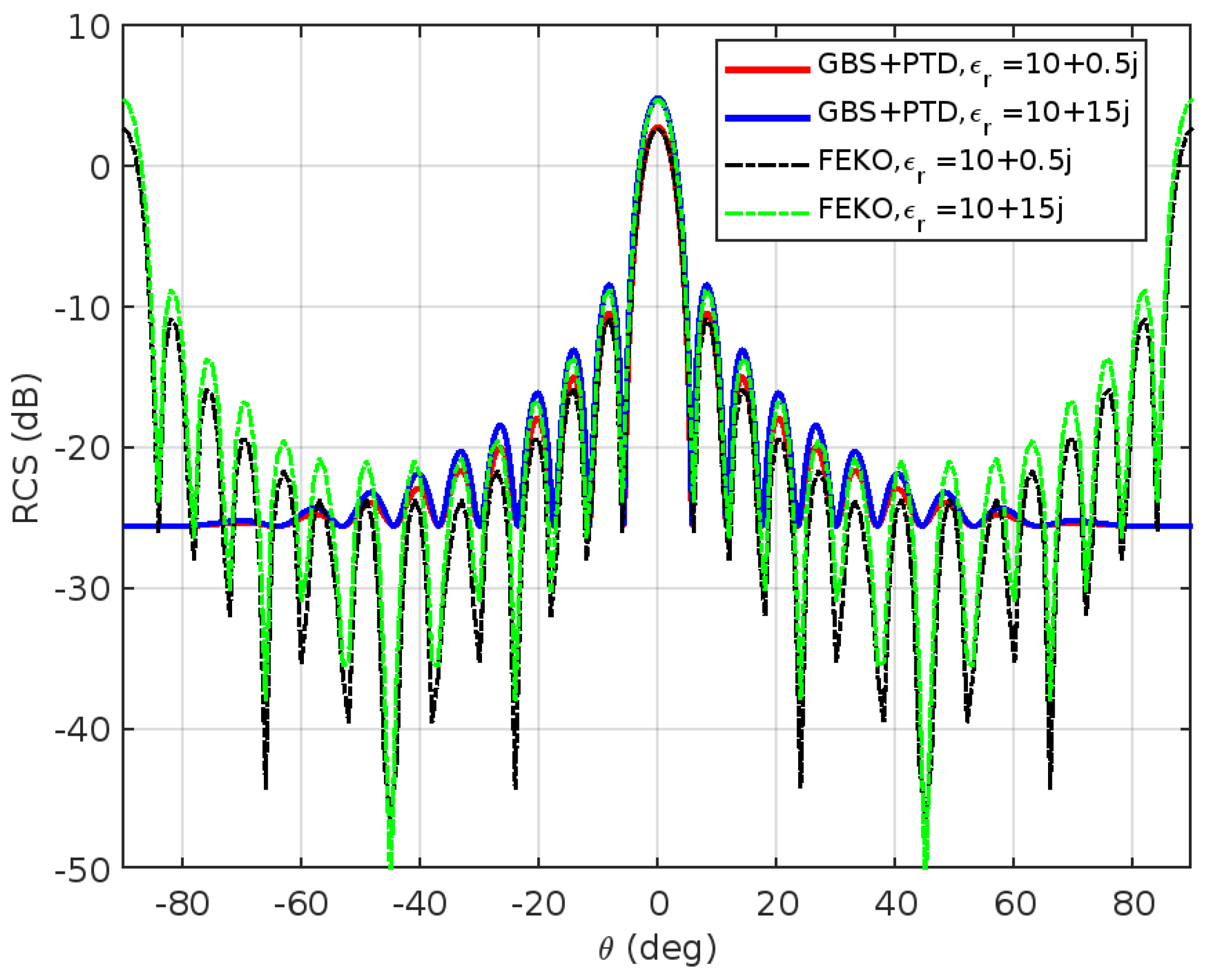
3.3.2. Exploring a Different Frequency Range

In this study, we aim to broaden our understanding by examining the impact of a different frequency on the results of the GBS method. Throughout this article, we have exclusively focused on a frequency of 10 GHz. However, we recognize the importance of exploring the behavior and characteristics at a different frequency range. By testing an alternative frequency, we seek to gain insights into how the results adapt to a different frequency.

In this investigation, we have chosen a frequency of 6 GHz, which falls within the C-band range, to examine the RCS of a rectangular plate. The plate has dimensions of $20\times 20$ cm${}^2$, and its permittivity is set to 1.5. The computational parameters for the GBS method are N = 1200 and r = 120.

Figure 15 illustrates a comparison of the results obtained using the GBS method and those obtained using the PO approximation and FEKO. The GBS results demonstrate a perfect agreement with those of FEKO within the angle range of $-20$ to 20 degrees. However, a slight difference becomes apparent as the angle increases beyond this range. This difference becomes more pronounced at higher angles of incidence (>50${}^{\circ }$), indicating the presence of some divergences between the GBS and PO methods on the one hand, and the FEKO method on the other.

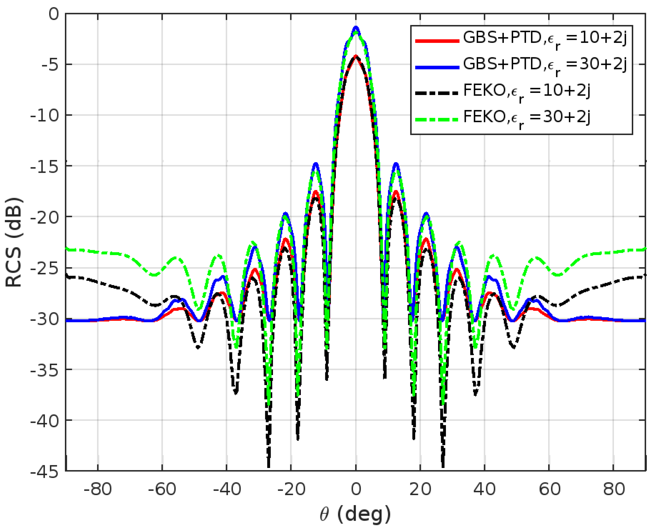
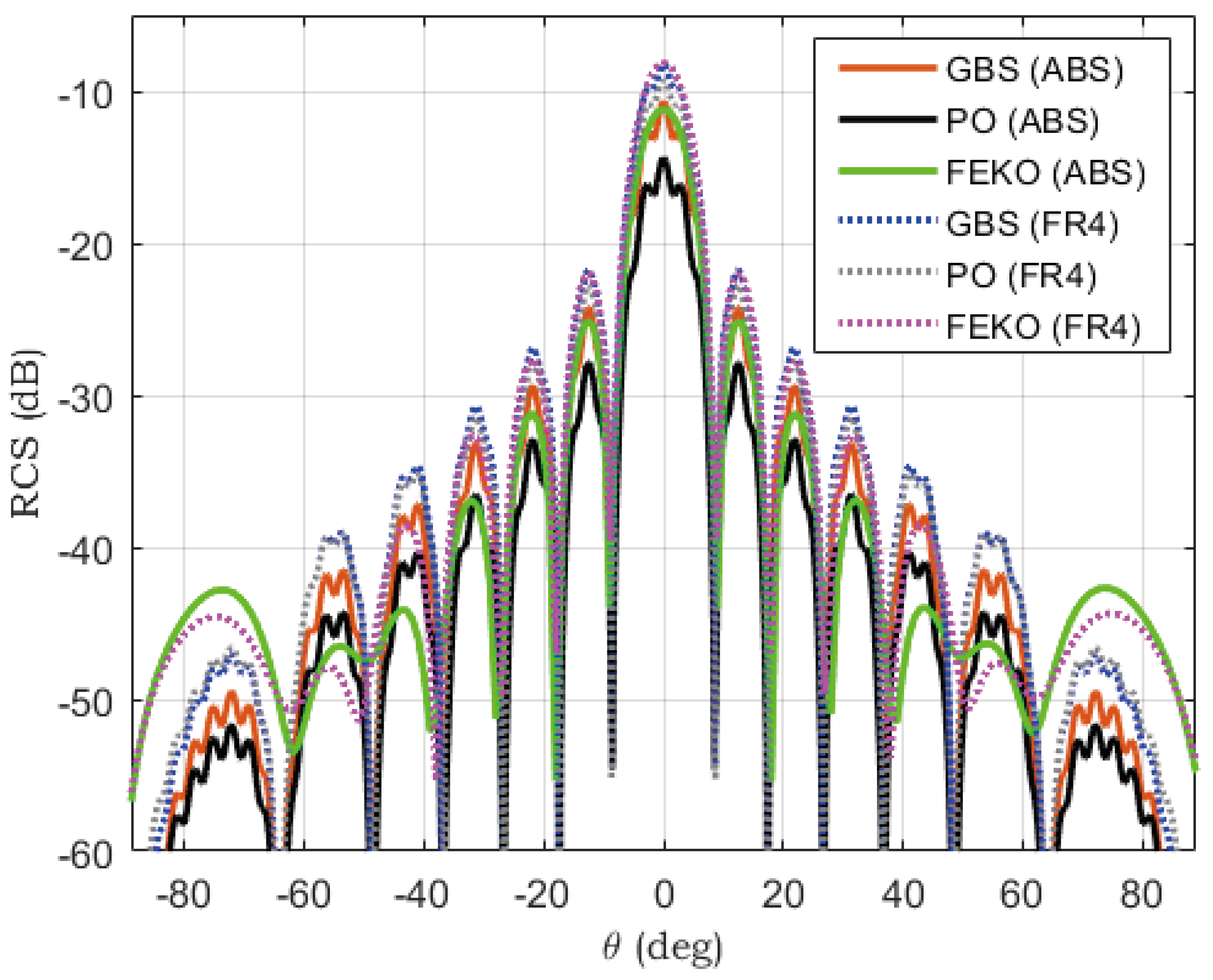
3.3.3. Numerical Validation with Existing Materials

In this section, we numerically validate the GBS method using existing dielectric materials. To conduct this numerical validation, we have chosen to compute the RCS of two dielectric materials, namely FR4 and ABS. FR4 is a type of epoxy laminate reinforced with glass fibers that is widely used in the production of electronics, specifically, printed circuit boards (PCBs), due to its exceptional electrical properties and durability. Moreover, it is preferred in the aerospace industry because of its lightweight and high-strength features. The term “FR4” implies that it meets fire safety standards and stands for “Flame Retardant 4”. FR4 can be tailored to fit specific design needs and is available in a variety of thicknesses. Its dielectric constant ranges from 3.9 to 4.6 depending on its composition and frequency, making it ideal for high-frequency applications such as PCBs and antennas [43].

In contrast, ABS is a thermoplastic polymer that is renowned for its durability, toughness, and resistance to impact and heat. It is frequently employed in the production of various consumer goods such as toys, electronic housing, and automotive parts. ABS also possesses excellent optical qualities, which makes it an ideal material for creating optical components like lenses [44]. ABS lenses find applications in several domains, such as diffraction or focusing light in optical systems. They are particularly useful in virtual and augmented reality applications, whereas focusing lenses are commonly utilized in cameras and projectors. The permittivity of ABS is dependent on its composition and frequency and typically ranges from 2.3 to 3.5, making it an excellent low-dielectric constant material for high-frequency applications. Hence, accurately characterizing the RCS values of both FR4 and ABS is essential for the optimization and design of radar systems in various sectors, including aerospace, defense, and telecommunications.

Furthermore, we propose to calculate the RCS of two identical targets with dimensions of $10\times 10\times 0.5$ cm${}^3$ and permittivity values of $4+0.00075j$ for FR4 and $2.6+0.005j$ for ABS. It should be noted that the imaginary parts of the permittivity of the two materials in question correspond to common values. The calculations are performed at 10 GHz with $N=900$ and $r=100$.

Figure 16 illustrates a comparison between the RCS of ABS and RF4 using three different methods: GBS, PO, and FEKO. The curves representing the RCS of FR4 (represented by the dotted lines) are consistently above the curves representing the RCS of ABS (represented by the solid lines) across a wide range of angles for all three methods. This suggests that ABS is a more suitable material for stealth applications than FR4 and is likely to produce weaker radar echoes when illuminated by electromagnetic radiation. The differences in the RCS between the two materials can be attributed to their different electromagnetic properties, such as permittivity. It is important to consider these differences when selecting materials for radar applications, as they can have a significant impact on system performance. Overall, the results of this comparison demonstrate the importance of accurate RCS calculations for understanding and optimizing radar systems.

A validation project is scheduled to confirm the accuracy of the GBS method simulation results in characterizing dielectric materials like FR4 and ABS. The project involves carrying out RCS measurements in an anechoic chamber and comparing the obtained results with simulated values to ensure the accuracy and reliability of our method. This will expand options for future research and development.

4. Discussion and Conclusions

In this paper, the GBS method is used in the context of radar applications, specifically for the prediction of the scattering properties of a given target. The theoretical formulation of the Gaussian beam summation technique allows for the calculation of the field in a homogeneous medium in three phases. In the first stage, a sufficiently dense ray tracing is performed from the source. Simultaneously, the calculation of the trajectories is performed step by step by numerically solving the dynamic ray-tracing system with the appropriate initial conditions. This step involves finding the coordinates of the observation point (neighboring ray) in the local reference frame, allowing us to determine the curvature of the wavefront and the amplitude profile of the Gaussian function. The third step involves summing all the contributions from the different rays propagating in the vicinity of the main ray by intercepting the receiver. For dielectric targets, we formulate the integral solution, whose complex weighting function is calculated by comparing the OP extended to the study of dielectric targets with that obtained by the fast descent path method. The assumed dielectric properties of the dielectric targets are taken into account by the Fresnel reflection coefficients, which are contained in the weighting function $\mathsf{\Phi }$. This integral is later discretized for the numerical solution.

The key benefit of this method is that it provides a very fast modeling methodology with excellent accuracy and efficiency for canonical targets. However, it can be extended to model a complex radar target by assembling a collection of relatively simple shapes such as flat plates, cylinders, etc. The target’s total RCS can be obtained as a coherent sum of the individual contributions.

Simulation results are presented to verify the efficiency and accuracy of the proposed method. The results are compared with those of FEKO using the ray-tracing approach and the extended formulation of the PO approximation for dielectric targets. The results show a good match in the specular direction. As the scattering direction moves farther away from the specular area, the Physical Optics and Gaussian Beam Summation predictions fail by steadily wider margins.

The edge returns can be more accurately predicted in the non-specular regions using PTD. This is because surface effects decrease to edge effect levels, and the edge contribution is not well modeled in PO and GBS. Indeed, induced currents are integrated over the illuminated parts of the body to obtain the far scattered fields. When applied to smooth bodies such as flat plates, the PO method may lead to erroneous contributions due to the abrupt discontinuity of the assumed surface fields at the shadow boundaries. The application of the first-order PTD version of elementary edge waves, which is free from the grazing singularity, provides a significant improvement over large aspect angles in the estimation of the RCS. However, it is necessary to include multiple diffraction coefficients to account for the multiple internal bounces and side surface effects when the thickness of the scattering targets is large. This aspect, when the thickness increases, will be pursued in future research.

In this paper, we focus on the calculation of the RCS in the mono-static configuration of conductive and dielectric targets. The bi-static configuration will be the subject of another paper since the GBS formulation used allows for easy switching from the mono-static to the bi-static configuration.

References

1. Burkholder, R.; Tokgoz, C.; Reddy, C.J.; Coburn, W.O. Iterative physical optics for radar scattering predictions. ACES J. 2009, 24, 241–258. [Google Scholar]
2. Hwang, J.-T.; Hong, S.-Y.; Song, J.-H.; Kwon, H.-W. Radar Cross Section analysis using physical optics and its applications to marine targets. J. Appl. Math. Phys. 2015, 3, 166–171. [Google Scholar] [CrossRef] [Green Version]
3. Hamel, P.; Adam, J.P.; Kubické, G.; Pouliguen, P. Design of a stealth wind turbine. In Proceedings of the Loughborough Antennas & Propagation Conference (LAPC), Loughborough, UK, 12–13 November 2012. [Google Scholar]
4. Dorn, O.; Lesselier, D. Level set methods for inverse scattering. Inverse Probl. 2006, 22, R67. [Google Scholar] [CrossRef] [Green Version]
5. Gibson, W.C. The Method of Moments in Electromagnetics; Chapman and Hall/CRC: Boca Raton, FL, USA, 2021. [Google Scholar]
6. Deschamps, G.A. Ray techniques in electromagnetics. Proc. IEEE 1972, 60, 1022–1035. [Google Scholar] [CrossRef] [Green Version]
7. Nieto-Vesperinas, M. Scattering and Diffraction in Physical Optics, 2nd ed.; World Scientific Publishing: Singapore, 2006. [Google Scholar]
8. Bennett, C.A. Principles of Physical Optics; John Wiley & Sons: Hoboken, NJ, USA, 2022. [Google Scholar]
9. Luneburg, R.K. Mathematical Theory of Optics; University of California Press: Berkeley, CA, USA, 1966. [Google Scholar]
10. Harrington, R.F. Time-Harmonic Electromagnetic Fields; IEEE Press: New York, NY, USA, 2001. [Google Scholar]
11. Oodo, M.; Murasaki, T.; Ando, M. Errors of physical optics in shadow region-fictitious penetrating rays. IEICE Trans. Electron. 1994, 77, 995–1004. [Google Scholar]
12. Keller, J.B. A geometrical theory of diffraction. In Calculus of Variations and Its Applications; McGraw-Hill: New York, NY, USA, 1958. [Google Scholar]
13. Levy, B.R. Diffraction by a Smooth Object; New York University, Graduate School: New York, NY, USA, 1958. [Google Scholar]
14. Kouyoumjian, R.G.; Pathak, P.H. A uniform geometrical theory of diffraction for an edge in a perfectly conducting surface. Proc. IEEE 1974, 62, 1448–1461. [Google Scholar] [CrossRef] [Green Version]
15. Kouyoumjian, R.G.; Pathak, P.H.; Burnside, W.D. A uniform GTD for the diffraction by edges vertices and convex surfaces. In Theoretical Methods for Determining the Interaction of Electromagnetic Waves with Structures; Sijthoff and Noordhoff: Amsterdam, The Netherlands, 1981; pp. 497–561. [Google Scholar]
16. Pathak, P.H. An asymptotic analysis of the scattering of plane waves by a smooth convex cylinder. Radio Sci. 1979, 14, 419–435. [Google Scholar] [CrossRef]
17. Ufimtsev, P.Y. Fundamentals of the Physical Theory of Diffraction; John Wiley & Sons: Hoboken, NJ, USA, 2014. [Google Scholar]
18. Ufimtsev, P.Y. Elementary edge waves and the physical theory of diffraction. Electromagnetics 1991, 11, 125–160. [Google Scholar] [CrossRef]
19. Popov, M.M. A new method of computation of wave fields using Gaussian beams. Wave Motion 1982, 4, 85–97. [Google Scholar] [CrossRef]
20. Cerveny, V. Gaussian beam synthetic seismograms. J. Geophys. 1985, 58, 44–72. [Google Scholar]
21. Levy, M. Parabolic Equation Methods for Electromagnetic Wave Propagation; IEE: London, UK, 2000. [Google Scholar]
22. White, B.S.; Norris, A.; Bayliss, A.; Burridge, R. Some remarks on the Gaussian beam summation method. Geophys. J. Int. 1987, 89, 579–636. [Google Scholar] [CrossRef]
23. Chou, H.-T.; Pathak, P.H.; Burkholder, R.J. Novel Gaussian beam method for the rapid analysis of large reflector antennas. IEEE Trans. Antennas Propag. 2001, 49, 880–893. [Google Scholar] [CrossRef]
24. Lugara, D.; Letrou, C.; Shlivinski, A.; Heyman, E.; Boag, A. Frame-based Gaussian beam summation method: Theory and applications. Radio Sci. 2003, 38, 27. [Google Scholar] [CrossRef]
25. Fluerasu, A.; Letrou, C. Gaussian beam launching for 3D physical modeling of propagation channels. Ann. Telecommun. 2009, 64, 763–776. [Google Scholar] [CrossRef]
26. L’Hour, C.-A.; Fabbro, V.; Chabory, A.; Sokoloff, J. 2-D propagation modeling in inhomogeneous refractive atmosphere based on gaussian beams part i: Propagation modeling. IEEE Trans. Antennas Propag. 2019, 67, 5477–5486. [Google Scholar] [CrossRef]
27. Leye, P.O.; Khenchaf, A.; Pouliguen, P. Gaussian beam summation method vs. gaussian beam launching in high-frequency rcs of complex radar targets. In Proceedings of the 2016 IEEE International Geoscience and Remote Sensing Symposium (IGARSS), Beijing, China, 10–15 July 2016; pp. 2630–2633. [Google Scholar]
28. Leye, P.O.; Khenchaf, A.; Pouliguen, P. RCS complex target, Gaussian beam summation method. In Proceedings of the EUCAP 2016, Davos, Switzerland, 10–15 April 2016. [Google Scholar]
29. Leye, P.O.; Khenchaf, A.; Pouliguen, P. The Gaussian beam summation and the gaussian launching methods in scattering problem. J. Electromagn. Anal. Appl. 2016, 8, 219. [Google Scholar] [CrossRef] [Green Version]
30. Kaissar Abboud, M.; Khenchaf, A.; Pouliguen, P. Gaussian beams formalism for high frequency scattering problems by metallic targets. In Proceedings of the IEEE Conference on Antenna Measurments and Applications, (CAMA 2021), Antibes Juan-les-Pins, France, 15–17 November 2021. [Google Scholar]
31. Stratton, J.A.; Chu, L.J. Diffraction theory of electromagnetic waves. Phys. Rev. 1939, 56, 99. [Google Scholar] [CrossRef]
32. Guo, L.-X.; Jiao, L.-C.; Wu, Z.-S. Electromagnetic scattering from two-dimensional rough surface using the Kirchhoff approximation. Chin. Phys. Lett. 2001, 18, 214. [Google Scholar]
33. Mohammadzadeh, H.; Nezhad, A.Z.; Firouzeh, Z.H. Modified Physical Optics approximation for RCS calculation of electrically large objects with coated dielectric. J. Electr. Comput. Innov. JECEI 2015, 3, 115–122. [Google Scholar] [CrossRef]
34. Hill, N.R. Gaussian beam migration. Geophysics 1990, 55, 1416–1428. [Google Scholar] [CrossRef]
35. Erdelyi, A. Asymptotic representations of Fourier integrals and the method of stationary phase. J. Soc. Ind. Appl. Math. 1955, 3, 17–27. [Google Scholar] [CrossRef]
36. Cerveny, V.; Popov, M.M.; Psencik, I. Computation of wave fields in inhomogeneous media—Gaussian beam approach. J. R. Astron. Soc. 1982, 70, 109–128. [Google Scholar] [CrossRef] [Green Version]
37. Schelkunoff, S.A. On diffraction and radiation of electromagnetic waves. Phys. Rev. 1939, 56, 308. [Google Scholar] [CrossRef]
38. Norris, A.N. Complex point-source representation of real point sources and the Gaussian beam summation method. JOSA A 1986, 3, 2005–2010. [Google Scholar] [CrossRef]
39. Horwitz, A. A generalization of Simpson’s rule. Approx. Theory Its Appl. 1993, 9, 71–80. [Google Scholar]
40. Nguyen, A.; Shirai, H. Electromagnetic scattering analysis from rectangular dielectric cuboids-TE polarization. IEICE Trans. Electron. 2016, 99, 11–17. [Google Scholar] [CrossRef]
41. Quang, H.N.; Shirai, H. High frequency plane wave scattering analysis from dielectric cuboids—TM polarization. In Proceedings of the 2017 XXXIInd General Assembly and Scientific Symposium of the International Union of Radio Science (URSI GASS), Montreal, QC, Canada, 19–26 August 2017; pp. 1–4. [Google Scholar] [CrossRef]
42. Apaydin, G.; Hacivelioglu, F.; Sevgi, L.; Gordon, W.B.; Ufimtsev, P.Y. Diffraction at a rectangular plate: First-order PTD approximation. IEEE Trans. Antennas Propag. 2016, 64, 1891–1899. [Google Scholar] [CrossRef]
43. Murugesan, A.; Natarajan, D.; Selvan, K.T. Low-Cost, Wideband Checkerboard Metasurfaces for Monostatic RCS Reduction. IEEE Antennas Wirel. Propag. Lett. 2021, 20, 493–497. [Google Scholar] [CrossRef]
44. Furlan, W.D.; Ferrando, V.; Monsoriu, J.A.; Zagrajek, P.; Czerwińska, E.; Szustakowski, M. 3D printed diffractive terahertz lenses. Opt. Lett. 2016, 41, 1748–1751. [Google Scholar] [CrossRef] [Green Version]
Figure 1. Schematic representation of the problem.
Remotesensing 15 03663 g001
Figure 2. New ray-centered coordinate system ( s , n ) around the ray Γ 0 .
Remotesensing 15 03663 g002
Figure 3. Schematic representation of the problem for a dielectric facet.
Remotesensing 15 03663 g003
Figure 4. Variation in the amplitude of the field for different values of the beam width with a fixed number of beams N ( N = 81 ).
Remotesensing 15 03663 g004
Figure 5. RCS at 10 GHz of a flat circular plate with a radius a = 7.5 cm (2a = 5 λ ).
Remotesensing 15 03663 g005
Figure 6. RCS at 10 GHz of a flat circular plate with a radius a = 15 cm (2a = 10 λ ).
Remotesensing 15 03663 g006
Figure 7. The geometry of the cuboid.
Remotesensing 15 03663 g007
Figure 8. RCS at 10 GHz from the top surface of a thin cuboid, ϵ r = 20 + 2 j ; 2a = 2b = 5 cm ( 2 a = 2 b = 1.6 λ ) ; 2c = 0.5 cm ( c = 0.16 λ ) .
Remotesensing 15 03663 g008
Figure 9. RCS at 10 GHz from the top surface of a thin cuboid, ϵ r = 20 + 2 j ; 2a = 2b = 10 cm ( 2 a = 2 b = 3.33 λ ) ; 2c = 1 cm ( 2 c = 0.33 λ ) .
Remotesensing 15 03663 g009
Figure 10. RCS at 10 GHz from the top surface of a thin cuboid with various real parts of permittivity and dimensions of 2a = 2b = 10 cm ( 2 a = 2 b = 3.33 λ ) ; 2c = 1 cm ( 2 c = 0.33 λ ) .
Remotesensing 15 03663 g010
Figure 11. RCS at 10 GHz from the top surface of two different cuboids with various imaginary parts of permittivity and dimensions of 2 a = 2 b = 15 cm ( 2 a = 2 b = 5 λ ) ; 2 c = 0.5 cm ( 2 c = 0.17 λ ) .
Remotesensing 15 03663 g011
Figure 12. RCS at 10 GHz from the top surface of two different cuboids with various imaginary parts of permittivity and dimensions of 2 a = 2 b = 15 cm ( 2 a = 2 b = 5 λ ) ; 2 c = 10 cm ( 2 c = 3.33 λ ) .
Remotesensing 15 03663 g012
Figure 13. Computation time vs. N.
Remotesensing 15 03663 g013
Figure 14. Relative error vs. N.
Remotesensing 15 03663 g014
Figure 15. RCS at 6 GHz of a dielectric rectangular plate with dimensions of 2 a = 2 b = 20 cm ( 2 a = 2 b = 4 λ ) .
Remotesensing 15 03663 g015
Figure 16. Comparison of RCS calculations for RF4 and ABS materials using GBS, PO, and FEKO.
Remotesensing 15 03663 g016